Particles, string and interface
in the three-dimensional Ising model
Gesualdo Delfino1,2, Walter Selke3 and Alessio Squarcini4,5
1SISSA – Via Bonomea 265, 34136 Trieste, Italy
2INFN sezione di Trieste, 34100 Trieste, Italy
3Institute for Theoretical Physics, RWTH Aachen University, 52056 Aachen, Germany
4Max-Planck-Institut für Intelligente Systeme,
Heisenbergstr. 3, D-70569, Stuttgart, Germany
5IV. Institut für Theoretische
Physik, Universität Stuttgart, Pfaffenwaldring 57, D-70569
Stuttgart, Germany
We consider the three-dimensional Ising model slightly below its critical temperature, with boundary conditions leading to the presence of an interface. We show how the interfacial properties can be deduced starting from the particle modes of the underlying field theory. The product of the surface tension and the correlation length yields the particle density along the string whose propagation spans the interface. We also determine the order parameter and energy density profiles across the interface, and show that they are in complete agreement with Monte Carlo simulations that we perform.
1 Introduction
The notion of interface plays an important role in different areas of physics. In statistical systems, the separation of different phases is characterized through the formation of an interface. In particle physics, the simplest description of confinement is in terms of a flux tube (a string) that connects the quarks and whose time propagation spans an interface. Lattice discretization establishes a direct connection between the two problems when duality relates a spin model to a lattice gauge theory, with the Ising model providing the basic example [1]. Effective descriptions adopting interfacial fluctuations as the basic degrees of freedom result into capillary wave theory [2] on one side, and effective string actions [3, 4] on the other.
In this paper we consider the three-dimensional Ising model in its scaling limit below the critical temperature , where it is described by field theory, and use the asymptotic particle states of the bulk field theory as the basis on which to perform expansions in momentum space. Introducing boundary states that induce the presence of an interface, the formalism allows us to determine the interfacial properties, including the magnetization and energy density profiles at leading order in the linear size of the interface. We then numerically determine the profiles through Monte Carlo simulations for different values of the temperature and of the size , and exhibit complete agreement with the analytic results, in absence of adjustable parameters.
The paper is organized as follows. In the next section, we introduce the boundary state setup and use it to determine the interfacial free energy and the expression of one-point functions, from which we then obtain the magnetization and energy density profiles. Section 3 is devoted to Monte Carlo simulations of the near-critical Ising model on the cubic lattice and to comparison with the analytic results for the profiles. Finally, in section 4 we discuss several implications of our results and point out lines of further development.
2 From particles to the interface
We consider the Ising model with reduced Hamiltonian
| (1) |
where is the spin variable located at the site of a cubic lattice, and the sum is performed over all pairs of nearest neighboring sites. We focus on the case of temperatures , in which the spin reversal symmetry of the Hamiltonian is spontaneously broken, i.e.
| (2) |
as usual, denotes the average over spin configurations weighted by . More precisely, we restrict our attention to the temperature range slightly below , where the correlation length becomes large and the system is described by a three-dimensional Euclidean field theory, which in turn is the continuation to imaginary time of a quantum field theory in dimensions. This amounts to consider the scaling region below , and our analytic results quantitatively hold as long as the temperature dependence of the observables is ruled by the Ising critical exponents. As we detail in section 3, this scaling regime is distant above the roughening transition temperature [5] below which the fluctuations of the interface are suppressed. In the continuum we will denote by a point in Euclidean space, being the imaginary time direction, and by the spin field. We refer to this translationally and rotationally invariant theory as the bulk theory.

We then focus on the case in which the system is finite in the direction, with and , while the size in the and directions is kept infinite in the theoretical analysis. The boundary conditions at are chosen in such a way that for and for ; the spins are left unconstrained for . It follows that for and large, the magnetization tends to the bulk value as , and to as ; we denote by configurational averages with the boundary conditions we have fixed. The two pure phases for large and negative and large and positive are separated around by an interfacial region spanned by the fluctuations of an interface running between the straight lines at (Figure 1). It is our goal to determine the expectation value of a field .
The fact that the scaling region around the critical temperature is described by a field theory is well known and widely used, in particular for the perturbative determination of the Ising critical exponents [1]. On the other hand, a field theory admits a particle description (see e.g. [6]), and it is this description that we will exploit for our study of the interface. Non-translationally invariant states of the system correspond to field theoretical states with nonzero energy and momentum. Energy and momentum are carried by the particles of the bulk field theory11 1 It is worth stressing that the particles we refer to throughout the paper describe the collective excitation modes of the system, and should not be confused with the individual molecules of a fluid whose near-critical properties are described by the field theory.. They evolve in two spatial dimensions (the and directions of Figure 1) and one imaginary time dimension (the direction). The analytic continuation to imaginary (or Euclidean) time is the usual way [1, 6] to exploit the fact that a near-critical statistical system at thermal equilibrium in spatial dimensions can be mapped onto a quantum system in spatial dimensions and one time dimension. In our case , and the rotational invariance (isotropy) of the statistical system in three Euclidean dimensions is mapped into relativistic invariance of the quantum system in dimensions. It follows that the energy of a particle mode with momentum and mass obeys the relativistic dispersion relation . The asymptotic -particle states of the bulk field theory provide a basis on which generic excitations of the system can be expanded. They are eigenstates of the energy and momentum operators with eigenvalues and , respectively.
The boundary conditions that we impose at correspond in the field theory to boundary states of the Euclidean time evolution, with denoting the energy operator (Hamiltonian) of the -dimensional quantum system. A boundary state can be expanded on the basis of asymptotic states of the bulk field theory. For our boundary conditions below , the boundary states correspond to an excitation (a string) extending for all values of , and whose propagation in the direction spans the interface. It follows that the number of particles entering the states in the expansion has to be extensive in the direction, and is therefore infinite. In order to regulate our expressions, we write this number as , and this limit will be understood in the following. We then write
| (3) |
where is an amplitude, particle states are normalized as , and the delta function enforces translation invariance in the direction. is the mass of the lightest particle in the spectrum of the spontaneously broken phase of the bulk field theory. It enters the large distance decay of the spin-spin correlator as . Comparison with the definition of the correlation length yields
| (4) |
States involving heavier particles also enter the expansion (3) in the part that we do not write explicitly. As we will immediately discuss, they produce only subleading corrections in the large limit we are interested in.
The partition function corresponding to our boundary conditions is given by the overlap between the two boundary states, which implements the sum over configurations of particles propagating between the bottom and top surfaces. Then we have
| (5) | |||||
where we used the fact that the large limit forces all momenta to be small, defined , exploited , and regularized as , so that here and in the following formulae is the size of the system in the direction. Here and below the symbol indicates omission of terms subleading for large . It appears from (5) how the contribution to of a state in which a particle of mass is replaced by one of mass is further suppressed at large by a factor .
The interfacial free energy, i.e. the contribution to the free energy due to the presence of the interface, is . The interfacial tension is defined as the interfacial free energy per unit area, , for both and going to infinity. Hence, it follows from (5) and (4) that it is given by22 2 Since the limit is understood, in (6) we only indicate the limit .
| (6) |
where
| (7) |
The reason for introducing is that, being dimensionless, it is a universal number, namely a number that near criticality is the same for different lattice discretizations. It also follows that , the number of particles per unit length along the string, can be written as ; equivalently, there are particles per correlation length in the direction. Notice that, since the energy of the state is the sum of the particle energies, in (3) the interaction among the particles is taken into account by the amplitude . In the large limit that we consider this function is projected to the constant , which only corresponds to the arbitrary normalization of the boundary state and can be set, in particular, to one. We deduce that the large limit is one of weakly interacting, and then (in average) widely separated, particles. This conclusion fully agrees with the fact that the known Monte Carlo value [7] corresponds to an average interparticle distance in the direction of about ten correlation lengths. It is particularly interesting that the particle description provides insight on a measurable and universal quantity like .
Notice also that, while and enter our formulae as regulators that go to infinity, measurable quantities like (6) only depend on the finite ratio (7). This internal consistency of the theory is further illustrated by the one-point functions (i.e. expectation values of local observables) that we now compute. It is also worth stressing how, since the initial expression (3) includes all fluctuations (sum over all particle excitations and all momenta), the large asymptotics that we derive are exact.
The one-point functions at are given by
| (8) | |||||
where we again consider the large limit, the vanishing of the component of the total momentum yields -independence, and the matrix element
| (9) | |||
is evaluated for small momenta. In the second line we take into account its decomposition in connected and disconnected parts, the latter originating from annihilation of particles on the left with particles on the right [6]; the subscript denotes connected matrix elements, and the dots indicate that all possible annihilations have to be included. It follows from (8) that each power of momentum in the integral contributes a factor to the one-point function. Since each annihilation in (9) produces a delta function , and then a factor , the leading contribution to (8) for large is obtained maximizing the number of annihilations. Since annihilations leave an -independent term , the interesting term is that with annihilations. Taking also into account that there are ways of performing annihilations, we finally obtain
| (10) |
If behaves as momentum to the power , the -dependent part of (10) behaves as
| (11) |
We also have that the integral term in (10) is even (resp. odd) in when is even (resp. odd) under exchange of and .
The fact that the magnetization profile has to be an odd function of interpolating between and fixes and . This leads to33 3 A suitable extension of (12) to generic small momenta appears to be . For it yields , and (12) is the way of extracting the sign from the square root compatible with the usual analyticity requirements [8] for the matrix elements, which do not allow for absolute values.
| (12) |
Upon insertion in (10) the pole in is conveniently canceled by differentiation with respect to . Performing the momentum integrations and integrating back in we obtain
| (13) |
| (14) |
and . The error function entering the magnetization profile (13) already appears in the exact result in two dimensions [9, 10, 11], a circumstance that we will discuss in section 4.
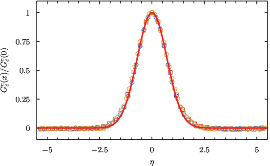
The energy density profile has to be an even function of , but the value of is not obvious a priori and remains as a parameter. We then write
| (15) |
The integrations in (10) are easily performed passing to the variables and yield the result
| (16) |
where we exploited the fact that the result must have the scaling dimension of the energy density field to express the temperature dependence of the prefactor of the Gaussian in terms of the correlation length; is then a dimensionless constant depending on the normalization of . Equation (14) shows that the width of the Gaussian in (16), i.e. the width of the interfacial fluctuations around the pinning position , is infinite for . This accounts for the vanishing of the magnetization profile (13) for : due to the infinite fluctuation width, the interface can be found with equal probability to the right or to the left of any point along the -axis, and the average yields a zero magnetization. However, for finite, no matter how large, translation invariance along the -axis is broken.
3 Comparison with Monte Carlo simulations
We now compare the theoretical predictions with Monte Carlo simulations of the Ising model on the simple cubic lattice. Most of the numerical data for the bulk quantities entering our analysis are given, for example, in [12] with an accuracy sufficient for our purposes. In particular, we have (corresponding to ), , . The critical exponents and rule the behavior of the correlation length and spontaneous magnetization for as (see e.g. [1])
| (17) | |||||
| (18) |
respectively. The critical amplitude can be obtained from a fit of the data listed in Table 3 of [12] and reads . For the bulk magnetization, the numerical approximation [13]
| (19) |
is available, which also estimates the first corrections to (18) for small and fits very well the data in the temperature range of our interest [12, 13].
We shall focus on the numerical determination, by Monte Carlo techniques, of the profiles for the magnetization and the energy density for which we derived the analytic expressions (13) and (16). The system is simulated on the simple cubic lattice in the volume , , , with sufficiently larger than in order to take into account that we want to compare with theoretical results corresponding to infinite . The boundary spins are fixed as previously described for , and are left free on the other boundaries.
As in our recent Monte Carlo simulations for two-dimensional Potts models [14] and three-dimensional XY model [15], the standard Metropolis algorithm [16] turned out to be useful. In particular, to test the predictions of the theory and to study finite size effects, we varied the lattice sizes and the temperature. The linear dimension ranged from 11 to 47, with ranging from 55 to 121 (the lengths are expressed in units of the lattice spacing). Data were taken at temperatures above the roughening transition, (see [17]), and below of the Ising model on the cubic lattice, concentrating on the region , where the bulk correlation length shows the scaling behavior (17). This is the scaling region in which the Monte Carlo results can be compared with our analytical results. Specifically, we analyzed the temperature interval between and 4.4. As usual, to obtain numerical results of high quality, we varied the length of the Monte Carlo runs, in between and Monte Carlo steps per site (MCS). Studying lattices of finite size below the critical point, we then performed simulations with MCS. Thermal averages were taken for the quantities of interest of the theory, the magnetization and energy density profiles in the center of the lattice. To test and determine the accuracy of the simulation data, we averaged over, at least, four independent Monte Carlo runs, using different random numbers in each realization. The resulting error bars normally did not exceed the size of the symbols in Figures 2 and 3, where final Monte Carlo results together with the theoretical predictions are shown.
The magnetization and the energy density are local observables and their determination below can be ordinarily performed as in the bulk case (see [12]). The difference in our case is that the boundary conditions that we adopt induce the -dependence that we determined in (13) and (16) starting from the particle description of the interface. The simulations are necessarily performed for finite, but for sufficiently larger than the Monte Carlo data are expected to reproduce the infinite analytical results (13) and (16), in which the profiles flatten on the constant bulk values for large. This is fully confirmed by the comparisons between theory and data in Figures 2 and 3.

The profiles are determined along the axis , with sufficiently far from the boundaries. Figure 2 shows that the Monte Carlo data that we obtain for the magnetization for different values of and exhibit the theoretically predicted collapse on a single curve once divided by and plotted as a function of the scaling variable (14). While the observation of this scaling behavior is in itself a notrivial confirmation of the theory, the figure also shows that the numerically determined profile agrees very well with the analytical result , see (13). It is worth stressing that the comparison contains no adjustable parameter.
For the energy density, which on the lattice corresponds to , with the sum running over the nearest neighbors of site , we consider the profile , which we obtain subtracting the plateau (bulk) value that we read from the data. Figure 3 shows that the Monte Carlo data for exhibit the expected collapse when plotted against ; agreement with the analytic result is also very good, again without free parameters.
It is worth stressing that, as confirmed by the comparison with Monte Carlo data in Figures 2 and 3, the results (13) and (16) are the answer to the specific problem that we studied, namely that of temperatures in the scaling region below and interpinning distance as the only finite size variable. These specifications correspond to the goal of this paper: describing the near-critical system with an interface starting from the particle modes of the bulk field theory, and doing so in an analytically exact way that allows for a parameter-free comparison with Monte Carlo simulations of the system on a lattice. Different system specifications are expected to lead to expressions for the profiles qualitatively similar to (13) and (16) from the point of view of the -dependence, but differing from them in the functional form and/or parameter dependence.
4 Discussion
In this paper we have considered the three-dimensional Ising model slightly below the critical temperature , with boundary conditions enforcing the presence of an interface running between two straight lines separated by a distance much larger than the bulk correlation length . We have shown analytically how the interface emerges from the study of the bulk field theory supplemented with the required boundary conditions. In particular, we showed how the string whose imaginary time propagation spans the interface is related to the particle modes of the field theory, and how the interfacial tension is expressed in terms of the particle density along the string. We then determined the order parameter and energy density profiles, and exhibited the complete agreement of these analytical results with the Monte Carlo simulations that we performed.
The analytic derivation was performed within the field theory that describes the scaling limit of the three-dimensional Ising model in its broken phase. As usual, this limit is described by the field theory in the vicinity of its nontrivial renormalization group fixed point [1]. We exploited the particle description of this field theory, in which the particles describe the near-critical excitation modes. We showed that in the large limit that we considered the interfacial fluctuations are produced by particles that are in average largely separated, and then weakly interacting. This allowed us to obtain the exact large results (13) and (16), in which the information (critical exponents and amplitudes) associated to the nontrivial fixed point is contained in the magnetization and correlation length as specified by (17) and (18). We could then rely on the numerical values of the critical data available in the literature to perform the parameter-free comparison between analytic and Monte Carlo results shown in Figures 2 and 3.
The theoretical derivation shows that the interface exhibits Gaussian fluctuations that are not due to displacements of the interface as a whole (which would require an infinite amount of energy), but to localized excitations that, at leading order in , involve single-particle modes44 4 Multi-particle modes yielding subleading terms in can also be derived from (8).. These excitations propagate in the -dimensional space (both momentum components and are non-zero), but the configurational average distributes them along the surface in such a way to finally yield the translational invariance of the profiles in the direction required by the boundary conditions.
This mechanism, which involves the connectedness structure of the matrix elements of local fields on particle states, effectively implements a form of dimensional reduction in the large limit of the configurational average. This is why the magnetization profile (13) is analogous to that in two dimensions, i.e. in absence of the axis in Figure 1. The profile in two dimensions was obtained from the lattice solution of the Ising model in [9] (see also [10]), and more recently in field theory in [11]. The dimensional interplay holds up to an important difference: the factor in (14) is absent in two dimensions. The origin of this difference is easy to understand in field theory. In two dimensions the particle modes of the Ising model below have a topological nature – they are kinks [6] -- and the spin field couples only to topologically neutral states, of which the kink-antikink state is the lightest one55 5 This corresponds to the peculiar fact that the leading singularity in momentum space of the spin-spin correlation function of the two-dimensional Ising model below the critical temperature is a branch cut rather than a pole (see [18]). (see [19]). This is why in two dimensions the relation (4) is replaced by . It follows that in three dimensions the variance of the interfacial fluctuations expressed in terms of – the measurable length scale of the statistical system – is half of that in two dimensions.
The emergence of these mechanisms implies, in particular, the relevance in three dimensions of results recently obtained in two dimensions. These include those of [11] for the relation between subleading corrections in and the internal structure of the interface, those of [20, 21] for interfacial wetting [22], those of [23, 24, 25] for the effects of system geometry, and those of [26] for the long range correlations induced by the presence of the interface. The detailed investigation of these points will provide relevant directions of further development.
In the realm of mathematically rigorous results, the three-dimensional Ising model with the boundary conditions of Figure 1 has been constantly studied (see [27] and references therein) for sufficiently low temperatures (lower than the roughening temperature ) since the proof of the ”rigidity” of the interface in this regime [28]. In two dimensions, several properties of Ising interfaces have been proved in recent years, for in the Ornstein-Zernike framework (see [29] and references therein), and for [30] in the framework of Schramm-Loewner evolution (SLE) [31]. Our results may stimulate the mathematically rigorous investigation of the separation of phases in the three-dimensional Ising model for .
Acknowledgments. AS thanks SISSA for hospitality during the final stages of this work.
References
- [1] C. Itzykson and J.-M. Drouffe, Statistical Field Theory, vol. 1, Cambridge University Press, 1989.
- [2] F.P. Buff, R.A. Lovett and F.H. Stillinger Jr., Phys. Rev. Lett. 15 (1965) 621.
- [3] T. Goto, Prog. Theor. Phys. 46 (1971) 1560.
- [4] Y. Nambu, Phys. Rev. D 10 (1974) 4262.
- [5] G.D. Weeks, G.H. Gilmer and H.J. Leamy, Phys. Rev. Lett. 31 (1973) 549.
- [6] L.H. Ryder, Quantum Field Theory, Cambridge University Press, Second Edition, 1996.
- [7] M. Caselle, M. Hasenbusch and M. Panero, JHEP 09 (2007) 117.
- [8] R.J. Eden, P.V. Landshoff, D.I. Olive and J.C. Polkinghorne, The analytic S-matrix, Cambridge University Press, 1966.
- [9] D.B. Abraham, Phys. Rev. Lett. 47 (1981) 545.
- [10] D.B. Abraham, in Phase Transitions and Critical Phenomena, edited by C. Domb and J.L. Lebowitz, Vol. 10, p. 1, Academic Press, London, 1986.
- [11] G. Delfino and J. Viti, J. Stat. Mech. (2012) P10009.
- [12] M. Caselle and M. Hasenbusch, J. Phys. A 30 (1997) 4963.
- [13] A.L. Talapov and H.W.J. Blöte, J. Phys. A 29 (1996) 5727.
- [14] G. Delfino, W. Selke and A. Squarcini, J. Stat. Mech. (2018) 053203.
- [15] G. Delfino, W. Selke and A. Squarcini, Phys. Rev. Lett. 122, 050602 (2019).
- [16] D.P. Landau and K. Binder, A Guide to Monte Carlo Simulations in Statistical Physics, Cambridge University Press, 2005.
- [17] M. Hasenbusch and K. Pinn, Physica A 192 (1992) 342.
- [18] B.M. McCoy and T.T. Wu, Phys. Rev. D 18 (1978) 1259.
- [19] G. Delfino, J. Phys. A 37 (2004) R45.
- [20] G. Delfino and A. Squarcini, Annals of Physics 342 (2014) 171.
- [21] G. Delfino, JHEP 05 (2016) 032.
- [22] S. Dietrich, in Phase Transitions and Critical Phenomena, edited by C. Domb and J.L. Lebowitz, Vol. 12, p. 1, Academic Press, London, 1988.
- [23] G. Delfino and A. Squarcini, J. Stat. Mech. (2013) P05010.
- [24] G. Delfino and A. Squarcini, Phys. Rev. Lett. 113 (2014) 066101.
- [25] G. Delfino and A. Squarcini, Nucl. Phys. B 901 (2015) 430.
- [26] G. Delfino and A. Squarcini, JHEP 11 (2016) 119.
- [27] R. Gheissari and E. Lubetzky, arXiv:1901.04980
- [28] R.L. Dobrushin, Teor. Veroâtn. Primen., 17 (1972) 619.
- [29] D. Ioffe, S. Ott, Y. Velenik and V. Wachtel, arXiv:2001.04737.
- [30] D. Chelkak, H. Duminil-Copin, C. Hongler, A. Kemppainen and S. Smirnov, C.R. Math. 352 (2014) 157.
- [31] O. Schramm, Isr. J. Math., 118 (2000) 221.