跳到论文正文
W Papers独立论文阅读器 arXiv:1906.03135 论文正文 计算阅读时间 · 0%
引用这篇论文根据当前论文元数据生成,正式投稿前建议核对。


License: arXiv.org perpetual non-exclusive license
arXiv:1906.03135v2 [hep-th] 31 Jul 2019

On Conformal Blocks, Crossing Kernels and Multi-variable Hypergeometric Functions. The author belonged there until Mar. 2019.

Heng-Yu Chen1 and Hideki Kyono2 Affiliation: 1Department of Physics, National Taiwan University, Taipei 10617, Taiwan Affiliation: 2 Department of Physics, Kyoto University, Kitashirakawa Oiwake-cho, Kyoto 606-8502, Japan Affiliation:  heng.yu.chen@phys.ntu.edu.tw, hhh1567@gmail.com
Abstract

In this note, we present an alternative representation of the conformal block with external scalars in general spacetime dimensions in terms of a finite summation over Appell fourth hypergeometric function 𝐅4{{\bf{F}}}_{4}. We also construct its generalization to the non-local primary exchange operator with continuous spin and its corresponding Mellin representation which are relevant for Lorentzian spacetime. Using these results we apply the Lorentzian inversion formula to compute the so-called crossing kernel in general spacetime dimensions, the resultant expression can be written as a double infinite summation over certain Kampé de Fériet hypergeometric functions with the correct double trace operator singularity structures. We also include some complementary computations in AdS space, demonstrating the orthogonality of conformal blocks and performing the decompositions.

1 Introduction and Summary

Conformal blocks are fundamental building elements for constructing various correlation functions in conformal field theories, they allow us to disentangle the model-dependent dynamical CFT data from universal kinematical pieces constrained by conformal symmetries. Once the operator product expansion (OPE) channel is specified, we can expand conformal correlation functions in terms of conformal blocks, and the expansion coefficients are precisely the product of OPE coefficients. A similar situation occurs in elementary quantum mechanics, we expand arbitrary wave functions in terms of the eigenfunctions, which are often determined by the symmetries and the physical spectra of a given system, and the probability amplitudes describe the underlying dynamics. These eigenfunctions solve the appropriate Sturm-Liouville equations which ensure their orthogonality, moreover the corresponding equations can often be transformed into the defining differential equations of various well-known special functions.

It is natural to ask whether conformal blocks can also be systematically studied in the same vein, in other words, whether they arise as the eigenfunctions of suitable Sturm-Liouville type of equations? Are they orthogonal with respect to given integration measure, and can be connected with certain well-studied mathematical functions? The answers to these questions are affirmative. Various crucial ingredients have become available starting with the important work of Dolan and Osborn DO-2003, DO-2011, where a second order partial differential equation known as “quadratic Casimir equation”, determining the four-point global conformal blocks as a function of cross ratios was derived. The scaling dimension Δ\Delta and spin JJ of the exchange primary operator in the OPE governs the asymptotic behavior, and in even spacetime dimensions, compact solutions can be expressed in terms of Gauss hypergeometric functions F12{}_{2}F_{1}. For general spacetime dimensions, conformal blocks were given in terms of an infinite summation over Gegenbauer polynomials DO-2003 or more recently for three dimensions, where the expression is again an infinite summation over F12{}_{2}F_{1}s Hogervorst-2016. During these investigations, it was realized that conformal blocks share a close resemblance with a special class of two variable generalization of Jacobi polynomials studied extensively by Koornwinder and collaborators KoornwinderPapers. These polynomials are defined through a pair of commuting second and fourth order partial differential equations whose eigenvalues are labeled by two integers11 1 This operator was also recently considered in Fortin-2016a, Fortin-2019a in embedding space., and their orthogonality can be subsequently defined with known integration measure. In a related recent development Schomerus-2016, Chen-Qualls, it was shown that quadratic and quartic conformal Casimir operators can be mapped to linear combinations of two commuting conserved Hamiltonians of the trigonometric B​C2BC_{2} Calogero-Sutherland integrable system via a similarity transformation. The conformal blocks can therefore be directly identified with the explicit eigenfunctions of the B​C2BC_{2} Calogero-Sutherland system known as “Harish-Chandra functions” Schomerus1, which can again be expressed in terms of an infinite summation over hypergeometric functions.

Even when the explicit compact form of conformal blocks is available, integration involving them over spacetime coordinates or cross ratios still requires more diligence, as there are a few subtleties. First, because of the non-compactness of the conformal group, S​O​(1,d+1)SO(1,d+1) for Euclidean and S​O​(2,d)SO(2,d) for Lorentzian respectively, this means the eigenvalues for conformal Casimir operators are functions of continuous variables (Δ,J)(\Delta,J). This is similar to the scattering states in quantum mechanics which are generally non-normalizable. Second, the naive integration range often extends beyond the radius of OPE convergence for a given channel, additional analytic continuations are needed for the integral to be well-defined. Besides purely mathematical interests, obtaining an explicit and succinct form of conformal blocks and understanding their general properties also fits well with the conformal bootstrap program (See Reviews for reviews). Specifically, consider the crossing symmetry equation arises from expanding a single correlation function in terms of the basis for different OPE channels, in order to extract the OPE coefficients or to relate the spectra in different channels, we need to understand the orthogonality and analytic continuation to perform OPE inversion CH-2017, SSW-2017 or compute the corresponding mixing matrices known as the “crossing kernel” or “6j symbols” CrossingKernel-1, CrossingKernel-2, Liu-2018, Karateev-6J22 2 See also Mellin-Bootstrap1, Mellin-Crossing, Sleight-Taronna CK, Sleight-Taronna CK2 for a closely related computation of crossing kernels in the form of mixing coefficients among Mellin amplitudes.. In addition, it should be noted that we can consider large spin perturbation, i.e. when the spin of the exchange primary operator becomes large, we can recover the OPE data using the corresponding inversion formula for any twist and all orders from the double discontinuities in cross-ratio plane Alday.

In this note, we contribute some useful results in several directions towards this systematic study. In section 2, we provide an alternative expression for conformal block with integer spin exchange in general spacetime dimensions by considering its Mellin-Barnes representation Mack:2009, and showing that the integrated result can be written in a finite summation of Appell’s hypergeometric function 𝐅4{\bf F}_{4} over an integer partition33 3 It is interesting to note that similar multi-variable generalization of hypergeometric equations were also used to describe the propagation of scalar field in the integrable deformations of A​d​Sp×SpAdS_{p}\times S^{p} geometries Lunin-Papers. It was also brought to our attention after this work is completed, when study conformal correlation functions constrained by conformal Ward identities in the momentum space, expressions in terms of multi-variable hypergeometric functions can also naturally arise, as discussed in Coriano-Papers.. We demonstrate its validity by numerically matching it with known compact expressions in even dimensions and provide several other analytic checks and simplifications which can be useful for conformal bootstrap computations. We then further explicitly construct the conformal block for primary exchange operators with continuous spin by constructing a continuous version of the Mack polynomial or more appropriately named “Mack function”. The result can be expressed as linear combination of certain 𝔤Δ,J(s)​(z,z¯){\mathfrak{g}}^{({\rm{s}})}_{\Delta,J}(z,\bar{z}) functions given in (3) and its spin shadow transformation44 4 See also the earlier paper ChungI about constructing Lorentzian conformal blocks in a simpler setting.. These results provide us with the necessary ingredients for the computation of the crossing kernel in general spacetime dimensions in Section 4, where we applied the Lorentzian inversion formula derived in CH-2017 (see also SSW-2017). We demonstrate the final result can be written in terms of double integrals containing Kampé de Fériet functions, this representation is useful for us to identify the singularities associated with the double trace operators. Finally in section 5, we provide complementary computations by considering the holographic dual configurations for conformal partial waves in Anti de-Sitter (AdS) space, and demonstrate their orthogonality which can be understood as the orthogonality of AdS harmonic functions. We also consider some simple expansions in terms of these natural bases. In a few appendices, we provide some useful details about multi-variable hypergeometric functions and computation details.

2 Conformal Blocks with Integer Spin and Appell’s Hypergeometric Functions

In this note we will primarily focus on the four point correlation function of conformal field theories in general spacetime dimensions, which contain external scalar primary operators 𝒪Δi,0​(xi)=𝒪i​(xi){\mathcal{O}}_{\Delta_{i},0}(x_{i})={\mathcal{O}}_{i}(x_{i}) with scaling dimension Δi,i=1,2,3,4\Delta_{i},~i=1,2,3,4:

⟨∏i=14𝒪i​(xi)⟩=𝒯Δi(s)​(xi)​∑{𝒪Δ,J}λ12​𝒪​λ34​𝒪​GΔ,J(s)​(z,z¯).\left\langle\prod_{i=1}^{4}{\mathcal{O}}_{i}(x_{i})\right\rangle={\mathcal{T}}_{\Delta_{i}}^{({\rm{s}})}(x_{i})\sum_{\{{\mathcal{O}}_{\Delta,J}\}}\lambda_{12{\mathcal{O}}}\lambda_{34{\mathcal{O}}}\,G_{\Delta,J}^{({\rm{s}})}(z,\bar{z}). (1)

Here we have decomposed the correlation function into summation over the ss-channel exchange primary operator {𝒪Δ,J​(x)}\{{\mathcal{O}}_{\Delta,J}(x)\} and λ12​𝒪​λ34​𝒪\lambda_{12{\mathcal{O}}}\lambda_{34{\mathcal{O}}} are the product of OPE coefficients. Here we can further factor out the overall kinematic factor depending only on the external scaling dimensions {Δi}\{\Delta_{i}\}:

𝒯Δi(s)​(xi)=1(x122)Δ12+2​(x342)Δ34+2​(x142x242)a(s)​(x142x132)b(s),a(s)=Δ21−2,b(s)=Δ34−2,{\mathcal{T}}^{({\rm{s}})}_{\Delta_{i}}(x_{i})=\frac{1}{(x_{12}^{2})^{\frac{\Delta_{12}^{+}}{2}}(x_{34}^{2})^{\frac{\Delta_{34}^{+}}{2}}}\left(\frac{x_{14}^{2}}{x_{24}^{2}}\right)^{{\rm{a}}^{({\rm{s}})}}\left(\frac{x_{14}^{2}}{x_{13}^{2}}\right)^{{\rm{b}}^{({\rm{s}})}},\quad{\rm{a}}^{({\rm{s}})}=\frac{\Delta_{21}^{-}}{2},~~{\rm{b}}^{({\rm{s}})}=\frac{\Delta_{34}^{-}}{2}, (2)

and introduce the notation Δi​j±=(Δi±Δj)\Delta_{ij}^{\pm}=(\Delta_{i}\pm\Delta_{j}). The remaining function GΔ,J(s)​(z,z¯)G_{\Delta,J}^{({\rm{s}})}(z,\bar{z}) is called the s-channel conformal block which depends only on a pair of conformally invariant cross ratios (u,v)({\rm{u}},{\rm{v}}) or (z,z¯)(z,\bar{z}):

u=z​z¯=x122​x342x132​x242,v=(1−z)​(1−z¯)=x142​x232x132​x242,xi​j2=(xi−xj)2.{\rm{u}}=z\bar{z}=\frac{x_{12}^{2}x_{34}^{2}}{x_{13}^{2}x_{24}^{2}},~~{\rm{v}}=(1-z)(1-\bar{z})=\frac{x_{14}^{2}x_{23}^{2}}{x_{13}^{2}x_{24}^{2}},\quad x_{ij}^{2}=(x_{i}-x_{j})^{2}. (3)

In Euclidean spacetime ℝd{\mathbb{R}}^{d}, xi​j2≥0x_{ij}^{2}\geq 0 which implies u,v≥0{\rm{u}},{\rm{v}}\geq 0 or the cross ratios (z,z¯)(z,\bar{z}) are complex conjugate to each other z¯=z∗\bar{z}=z^{*}. While in Lorentzian spacetime 𝕄1,d−1{\mathbb{M}}^{1,d-1}, xi​j2x_{ij}^{2} can become negative instead, (z,z¯)(z,\bar{z}) are treated as independent complex variables in general, this distinction becomes important when we consider integration over the conformal blocks.

It is well known that the conformal block GΔ,J(s)​(z,z¯)G_{\Delta,J}^{({\rm{s}})}(z,\bar{z}) satisfies a so-called quadratic Casimir equation, which is a second order partial differential equation in (z,z¯)(z,\bar{z}) and is parameterized by (a(s),b(s))({\rm{a}}^{({\rm{s}})},{\rm{b}}^{({\rm{s}})})DO-2011:

(Dz​(a(s),b(s))+Dz¯​(a(s),b(s))+2​ε​z​z¯z−z¯​((1−z)​∂∂z−(1−z¯)​∂∂z¯))​GΔ,J​(z,z¯)=C2​(Δ,J)​GΔ,J​(z,z¯),\left(D_{z}({\rm{a}}^{({\rm{s}})},{\rm{b}}^{({\rm{s}})})+D_{\bar{z}}({\rm{a}}^{({\rm{s}})},{\rm{b}}^{({\rm{s}})})+2\varepsilon\frac{z\bar{z}}{z-\bar{z}}\left((1-z)\frac{\partial}{\partial z}-(1-\bar{z})\frac{\partial}{\partial\bar{z}}\right)\right)G_{\Delta,J}(z,\bar{z})=C_{2}(\Delta,J)G_{\Delta,J}(z,\bar{z}), (4)

where:

Dz​(a,b)=z2​(1−z)​d2d​z2−(1+a+b)​z2​dd​z−ab​z,h=d2,ε=h−1,D_{z}({\rm{a}},{\rm{b}})=z^{2}(1-z)\frac{d^{2}}{dz^{2}}-(1+{\rm{a}}+{\rm{b}})z^{2}\frac{d}{dz}-{\rm{a}}{\rm{b}}z,\quad h=\frac{d}{2},~~\varepsilon=h-1, (5)

and the eigenvalue C2​(Δ,J)C_{2}(\Delta,J):

C2​(Δ,J)=Δ⁡(Δ−d)+J⁡(J+d−2),C_{2}(\Delta,J)=\Delta(\Delta-d)+J(J+d-2), (6)

depends on the scaling dimension Δ\Delta and the spin JJ of the exchanged operator 𝒪Δ,J​(x){\mathcal{O}}_{\Delta,J}(x). It is interesting to note that treating (Δ,J)(\Delta,J) as parameters, the eigenvalue C2​(Δ,J)C_{2}(\Delta,J) has following three independent ℤ2{\mathbb{Z}}_{2} symmetry transformations:

Shadow:Δ⇔d−Δ,Spin Shadow:J⇔2−d−J,Light Ray:Δ⇔1−J,{\text{Shadow}}:\Delta\Leftrightarrow d-\Delta,~~~{\text{Spin Shadow}}:J\Leftrightarrow 2-d-J,~~~{\text{Light Ray}}:\Delta\Leftrightarrow 1-J, (7)

these imply that (4) has eight-fold degeneracies of independent eigenfunctions, only distinguished by their different asymptotic behaviors. The first one in (7) corresponds to the well-known shadow transformation introduced in DO-2011 which maps a local primary 𝒪Δ,J​(x){\mathcal{O}}_{\Delta,J}(x) to a non-local operator 𝒪~d−Δ,J​(x)\tilde{{\mathcal{O}}}_{d-\Delta,J}(x) with shadow scaling dimension d−Δd-\Delta via an integral transformation. The remaining two transformations in (7) generally map JJ to negative or even continuous values, as explained in details in LightRay (The close connection of these transformation with the Weyl group of B​C2BC_{2} group was also detailed in Schomerus1), these values can only be physical in Lorentzian instead of Euclidean spacetime. A primary operator 𝒪Δ,J​(x){\mathcal{O}}_{\Delta,J}(x) now transforms under S​O​(2,d)SO(2,d) instead of S​O​(1,d+1)SO(1,d+1), it is labeled by the two continuous Cartan numbers (Δ,J)(\Delta,J) of S​O​(1,1)Δ×S​O​(1,1)J∈S​O​(2,d)SO(1,1)_{\Delta}\times SO(1,1)_{J}\in SO(2,d), and they can be mixed under the Weyl group of S​O​(2,d)SO(2,d). It is useful to introduce here the spectral parameterization for Lorentzian spacetime:

Δ=h+i​ν,J=−ε+i​ℓ,\Delta=h+i\nu,\quad J=-\varepsilon+i\ell, (8)

such that the eigenvalue (6) can be rewritten as:

C2​(ν,l)=(h2+ν2)+(ε2+ℓ2).C_{2}(\nu,l)=(h^{2}+\nu^{2})+(\varepsilon^{2}+\ell^{2}). (9)

The transformations in (10) can be succinctly recast in terms of spectral parameters (ν,l)(\nu,l):

Shadow:ν⇔−ν,Spin Shadow:ℓ⇔−ℓ,Light Ray:ν⇔−ℓ,{\text{Shadow}}:\nu\Leftrightarrow-\nu,~~~{\text{Spin Shadow}}:\ell\Leftrightarrow-\ell,~~~{\text{Light Ray}}:\nu\Leftrightarrow-\ell, (10)

which clearly leave (9) invariant. We will return to these parameterizations when we consider the conformal block with continuous spin and the inversion formula of CH-2017.

In this note, we will ultimately be interested in constructing so-called “crossing kernel” for general dd-dimensional conformal field theories, which will be introduced momentarily. To begin with, we first construct an orthogonal basis in ℝd{\mathbb{R}}^{d} which will be called conformal partial wave (CPW) DO-2011:

Ψν,J(s)​(xi)=1πh​∫ℝddd​x0​⟨𝒪Δ1​(x1)​𝒪Δ2​(x2)​𝒪h+i​ν,Jμ1​…​μJ​(x0)⟩​⟨𝒪~h−i​ν,Jμ1​…​μJ​(x0)​𝒪Δ3​(x3)​𝒪Δ4​(x4)⟩.\Psi^{({\rm{s}})}_{\nu,J}(x_{i})=\frac{1}{\pi^{h}}\int_{\mathbb{R}^{d}}d^{d}x_{0}\langle{\mathcal{O}}_{\Delta_{1}}(x_{1}){\mathcal{O}}_{\Delta_{2}}(x_{2}){\mathcal{O}}_{h+i\nu,J}^{\mu_{1}...\mu_{J}}(x_{0})\rangle\langle\tilde{{\mathcal{O}}}_{h-i\nu,J}^{\mu_{1}...\mu_{J}}(x_{0}){\mathcal{O}}_{\Delta_{3}}(x_{3}){\mathcal{O}}_{\Delta_{4}}(x_{4})\rangle. (11)

Here the two copies of three point functions contain 𝒪h+i​ν,Jμ1​…​μJ​(x0){\mathcal{O}}_{h+i\nu,J}^{\mu_{1}\dots\mu_{J}}(x_{0}) and its shadow 𝒪~h−i​ν,Jμ1​…​μJ​(x0)\tilde{{\mathcal{O}}}_{h-i\nu,J}^{\mu_{1}\dots\mu_{J}}(x_{0}), they are related through following integral transformation:

𝒪~h−i​ν,μ1​…,μJ​(x)=1πh​Γ⁡(h−i​ν+J)(h+i​ν−1)J​Γ​(i​ν)​∫dd​x′​ℐμ1,…,μJ;ν1,…,νJ​(x−x′)((x−x′)2)h−i​ν​𝒪h+i​ν,ν1,…,νJ​(x′),\tilde{{\mathcal{O}}}_{h-i\nu,\mu_{1}\dots,\mu_{J}}(x)=\frac{1}{\pi^{h}}\frac{\Gamma(h-i\nu+J)}{(h+i\nu-1)_{J}\Gamma(i\nu)}\int d^{d}x^{\prime}\frac{{\mathcal{I}}_{\mu_{1},\dots,\mu_{J};\nu_{1},\dots,\nu_{J}}(x-x^{\prime})}{((x-x^{\prime})^{2})^{h-i\nu}}{\mathcal{O}}_{h+i\nu,\nu_{1},\dots,\nu_{J}}(x^{\prime}), (12)

where ℐμ1,…,μJ;ν1,…,νJ​(y){\mathcal{I}}_{\mu_{1},\dots,\mu_{J};\nu_{1},\dots,\nu_{J}}(y) is the inversion tensor of symmetric traceless tensors. The functional forms of these three point functions are fixed kinematically through conformal symmetry55 5 In this paper we follow the normalization convention of conformal partial wave Ψν,J(s)​(xi)\Psi_{\nu,J}^{({\rm{s}})}(x_{i}) explicitly constructed in DO-2011 by fusing two copies of three point functions together, this also fixes our expansion coefficients hence the normalization of conformal blocks.. Notice that the CPW is also an eigenfunction of the conformal Casimir equation and it can be expanded in terms of a conformal block and its shadow as follows:

Ψν,J(s)(xi)=𝒯Δi(s)(xi)∑σs=±𝐜h+i​σs​ν,J(s)Gh+i​σs​ν,J(s)(z,z¯)\Psi_{\nu,J}^{({\rm{s}})}(x_{i})={\mathcal{T}}^{({\rm{s}})}_{\Delta_{i}}(x_{i})\sum_{\sigma_{s}=\pm}{\bf{c}}_{h+i\sigma_{s}\nu,J}^{({\rm{s}})}G_{h+i\sigma_{s}\nu,J}^{({\rm{s}})}(z,\bar{z}) (13)

where the expansion coefficients are given by

𝐜h+i​σs​ν,J(s)=12J​cJ​(h−i​σs​ν−1)J​Γ​(−i​σs​ν)Γ⁡(2​ωσs)​Γ⁡(ωσs±a(s))​Γ​(ωσs±b(s))∏i=14Γ⁡(γi(s)),{\bf{c}}_{h+i\sigma_{s}\nu,J}^{({\rm{s}})}=\frac{1}{2^{J}c_{J}}\frac{(h-i\sigma_{s}\nu-1)_{J}\Gamma(-i\sigma_{s}\nu)}{\Gamma(2\omega_{\sigma_{s}})}\frac{\Gamma\left(\omega_{\sigma_{s}}\pm{\rm{a}}^{({\rm{s}})}\right)\Gamma\left(\omega_{\sigma_{s}}\pm{\rm{b}}^{({\rm{s}})}\right)}{\prod_{i=1}^{4}\Gamma\left(\gamma^{({\rm{s}})}_{i}\right)}, (14)

with cJ=(ε)J(2​ε)Jc_{J}=\frac{(\varepsilon)_{J}}{(2\varepsilon)_{J}} and (x)J=Γ⁡(x+J)Γ⁡(x)(x)_{J}=\frac{\Gamma(x+J)}{\Gamma(x)} being the Pochhammer symbol. In the above, we have also introduced the notation Γ⁡(x±a)=Γ⁡(x+a)​Γ​(x−a)\Gamma(x\pm a)=\Gamma(x+a)\Gamma(x-a). We have also defined the following combinations of scaling dimensions and spins:

ωσs=h+i​σs​ν+J2,τσs=h+i​σs​ν−J2,σs=±.\omega_{\sigma_{s}}=\frac{h+i\sigma_{s}\nu+J}{2},\quad\tau_{\sigma_{s}}=\frac{h+i\sigma_{s}\nu-J}{2},~~\sigma_{s}=\pm. (15)

while {γi(s)}\{\gamma_{i}^{({\rm{s}})}\} are given in (22). The integer spin-JJ operators 𝒪h+i​ν,J​(x0){\mathcal{O}}_{h+i\nu,J}(x_{0}) and 𝒪~h−i​ν,J​(x0)\tilde{{\mathcal{O}}}_{h-i\nu,J}(x_{0}) carry the complex scaling dimensions, we can recover the conformal block with physical real dimensions by integrating the conformal partial wave (13) over the ν\nu-plane together with the spectral function for ν\nu, see for example CKK:2017.

It is well-known that the conformal partial wave (13) also enjoys the Mellin representation DO-2011, Mack:2009:

Ψν,J(s)​(xi)=𝒯Δi(s)​(xi)​∫−i​∞i​∞d​s(4​π​i)​∫−i​∞i​∞d​t(4​π​i)​us2​vt2​ρΔi(s)​(s,t)​ℳν,J(s)​(s,t).{\Psi}_{\nu,J}^{({\rm{s}})}(x_{i})={\mathcal{T}}_{\Delta_{i}}^{({\rm{s}})}(x_{i})\int^{i\infty}_{-i\infty}\frac{ds}{(4\pi i)}\int^{i\infty}_{-i\infty}\frac{dt}{(4\pi i)}{\rm{u}}^{\frac{s}{2}}{\rm{v}}^{\frac{t}{2}}\rho^{({\rm{s}})}_{\Delta_{i}}(s,t){\mathcal{M}}^{({\rm{s}})}_{\nu,J}(s,t)\,. (16)

Here the Mellin space integration measure is given by:

ρΔi(s)​(s,t)=∏i<jΓ⁡(δi​j(s)),\rho^{({\rm{s}})}_{\Delta_{i}}(s,t)=\prod_{i<j}{\Gamma\left(\delta_{ij}^{({\rm{s}})}\right)}, (17)

where in principle we have three Mandelstam-like variables (s,t,u)(s,t,u) satisfying s+t+u=∑i=14Δis+t+u=\sum_{i=1}^{4}\Delta_{i}, such that we can substitute uu away and express {δi​j(s)}\{\delta_{ij}^{({\rm{s}})}\} only in terms of (s,t)(s,t):

δ12(s)=Δ12+−s2,δ34(s)=Δ34+−s2,δ13(s)=s+t2+b(s),δ24(s)=s+t2+a(s),δ14(s)=−t2−a(s)−b(s),δ23(s)=−t2,\delta_{12}^{({\rm{s}})}=\frac{\Delta_{12}^{+}-s}{2},~\delta_{34}^{({\rm{s}})}=\frac{\Delta_{34}^{+}-s}{2},~\delta_{13}^{({\rm{s}})}=\frac{s+t}{2}+{\rm{b}}^{(s)},~\delta_{24}^{({\rm{s}})}=\frac{s+t}{2}+{\rm{a}}^{(s)},~\delta_{14}^{({\rm{s}})}=-\frac{t}{2}-{\rm{a}}^{({\rm{s}})}-{\rm{b}}^{({\rm{s}})},~\delta_{23}^{({\rm{s}})}=-\frac{t}{2}, (18)

such that ∑j≠iδi​j(s)=Δi\sum_{j\neq i}\delta_{ij}^{({\rm{s}})}=\Delta_{i}. Notice the number of independent Mellin parameters is exactly the same as the independent cross ratios, we can regard the Mellin representation as trading (u,v)({\rm{u}},{\rm{v}}) with (s,t)(s,t). While the remaining integrand:

ℳν,J(s)​(s,t)=1∏i=14Γ⁡(γi(s))​Γ⁡(τ±−s2)Γ⁡(δ12(s))​Γ​(δ34(s))​Pν,J(s)​(s,t),{\mathcal{M}}^{({\rm{s}})}_{\nu,J}(s,t)=\frac{1}{\prod_{i=1}^{4}\Gamma\left(\gamma^{({\rm{s}})}_{i}\right)}\frac{\Gamma\left(\tau_{\pm}-\frac{s}{2}\right)}{\Gamma\left(\delta_{12}^{({\rm{s}})}\right)\Gamma\left(\delta_{34}^{({\rm{s}})}\right)}{P}_{\nu,J}^{({\rm{s}})}(s,t), (19)

is the corresponding ss-channel partial Mellin amplitude. The polynomial Pν,J(s)​(s,t){P}_{\nu,J}^{({\rm{s}})}(s,t) originally due to Mack Mack:2009 is given by:

Pν,J(s)​(s,t)=∑r,k~​(τ±−s2)r​∏(i​j)(δi​j(s))ki​j​∏i=14Γ⁡(γi(s))Γ⁡(γi(s)−J+r+∑jkj​i),{P}_{\nu,J}^{({\rm{s}})}(s,t)={\widetilde{\sum_{r,k}}}\left(\tau_{\pm}-\frac{s}{2}\right)_{r}\prod_{(ij)}{\left(\delta_{ij}^{({\rm{s}})}\right)_{k_{ij}}}\prod_{i=1}^{4}\frac{\Gamma\left(\gamma^{({\rm{s}})}_{i}\right)}{\Gamma\left(\gamma^{({\rm{s}})}_{i}-J+r+\sum_{j}k_{ji}\right)}, (20)

where the abridged double summations:

∑r,k~​⋯=J!2J​∑r=0⌊J2⌋(−1)r​(J+ε)−rr!​(J−2​r)!​∑∑ki​j=J−2​r(−1)k13+k24​(J−2​r)!∏(i​j)ki​j!​…{\widetilde{\sum_{r,k}}}\dots=\frac{J!}{2^{J}}\sum_{r=0}^{\left\lfloor\frac{J}{2}\right\rfloor}(-1)^{r}\frac{(J+\varepsilon)_{-r}}{r!(J-2r)!}\sum_{\sum k_{ij}=J-2r}(-1)^{k_{13}+k_{24}}\frac{(J-2r)!}{\prod_{(ij)}k_{ij}!}\dots (21)

is over rr which comes from the expansion coefficients of Gegenbauer polynomial arising from tensor contraction of three point functions, ⌊J2⌋\left\lfloor\frac{J}{2}\right\rfloor denotes integer part of J2\frac{J}{2} and the four-fold integer partition {ki​j}\{k_{ij}\} with (i​j)={13,24,14,23}(ij)=\{13,24,14,23\} such that ∑(i​j)ki​j=J−2​r\sum_{(ij)}k_{ij}=J-2r. The remaining parameters {γi(s)}\{\gamma_{i}^{({\rm{s}})}\} arising from the integration via Symanzik formula are given by:

γ1(s)=ω+−a(s),γ2(s)=ω++a(s),γ3(s)=ω−+b(s),γ4(s)=ω−−b(s).\gamma_{1}^{({\rm{s}})}=\omega_{+}-{\rm{a}}^{({\rm{s}})},~\gamma_{2}^{({\rm{s}})}=\omega_{+}+{\rm{a}}^{({\rm{s}})},~\gamma_{3}^{({\rm{s}})}=\omega_{-}+{\rm{b}}^{({\rm{s}})},~\gamma_{4}^{({\rm{s}})}=\omega_{-}-{\rm{b}}^{({\rm{s}})}. (22)

Despite the rather complicated looking expression for Pν,J(s)​(s,t){P}_{\nu,J}^{({\rm{s}})}(s,t) in (20), the most important analytic information we need about it is that it does not contain any additional singularities in (s,t)(s,t) variables, but only zeroes which cancel some of the poles in the (s,t)(s,t)-contour integrations. It is also useful to note that Mack polynomial (20) enjoys a somewhat non-obvious but important reflection symmetry Pν,J(s)​(s,t)=P−ν,J(s)​(s,t){P}^{({\rm{s}})}_{\nu,J}(s,t)={P}^{({\rm{s}})}_{-\nu,J}(s,t) ConfRegge, which is needed for consistently extracting the conformal block from integration over ν\nu-plane.

Using the Mellin representation of Ψν,J(s)​(xi)\Psi^{({\rm{s}})}_{\nu,J}(x_{i}) (16), we can readily integrate it into a summation over regularized Gauss Hypergeometric functions F~12{}_{2}\tilde{F}_{1}:

Ψν,J(s)​(xi)\displaystyle\Psi^{({\rm{s}})}_{\nu,J}(x_{i}) =\displaystyle= 𝒯Δi(s)(xi)∑σs=±∑r,k~∏i=141Γ⁡(γi(s)−J+r+∑jkj​i)uτσs+rva(s)+b(s)−k14−k232∑ns=0∞(−1)ns​unsns!Γ(−iσsν−ns)\displaystyle{\mathcal{T}}^{({\rm{s}})}_{\Delta_{i}}(x_{i})\sum_{\sigma_{s}=\pm}\widetilde{\sum_{r,k}}\prod_{i=1}^{4}\frac{1}{\Gamma\left(\gamma^{({\rm{s}})}_{i}-J+r+\sum_{j}k_{ji}\right)}\frac{{\rm{u}}^{\tau_{\sigma_{s}}+r}}{{\rm{v}}^{\frac{{\rm{a}}^{({\rm{s}})}+{\rm{b}}^{({\rm{s}})}-k_{14}-k_{23}}{2}}}\sum_{n_{s}=0}^{\infty}\frac{(-1)^{n_{s}}{\rm{u}}^{n_{s}}}{n_{s}!}\Gamma(-i\sigma_{s}\nu-n_{s}) (23)
×\displaystyle\times [vϖ14(s)2​𝐅~12​[κσs1​(s)+ns+r,κσs4​(s)+ns+r1+ϖ14(s);v]+vϖ23(s)2​𝐅~12​[κσs2​(s)+ns+r,κσs3​(s)+ns+r1+ϖ23(s);v]]\displaystyle\left[{\rm{v}}^{\frac{\varpi_{14}^{({\rm{s}})}}{2}}{}_{2}\tilde{\bf{F}}_{1}\left[\begin{matrix}~\kappa_{\sigma_{s}}^{1({\rm{s}})}+n_{s}+r,~\kappa_{\sigma_{s}}^{4({\rm{s}})}+n_{s}+r\\ ~1+\varpi^{({\rm{s}})}_{14}\end{matrix};{\rm{v}}\right]+{\rm{v}}^{\frac{\varpi_{23}^{({\rm{s}})}}{2}}{}_{2}\tilde{\bf{F}}_{1}\left[\begin{matrix}~\kappa_{\sigma_{s}}^{2({\rm{s}})}+n_{s}+r,~\kappa_{\sigma_{s}}^{3({\rm{s}})}+n_{s}+r\\ ~1+\varpi^{({\rm{s}})}_{23}\end{matrix};{\rm{v}}\right]\right]
=\displaystyle= 𝒯Δi(s)(xi)∑σs=±∑r,k~∏i=141Γ⁡(γi(s)−J+r+∑jkj​i)uτσs​ν+rva(s)+b(s)−k14−k232\displaystyle{\mathcal{T}}^{({\rm{s}})}_{\Delta_{i}}(x_{i})\sum_{\sigma_{s}=\pm}\widetilde{\sum_{r,k}}\prod_{i=1}^{4}\frac{1}{\Gamma\left(\gamma^{({\rm{s}})}_{i}-J+r+\sum_{j}k_{ji}\right)}\frac{{\rm{u}}^{\tau_{\sigma_{s}\nu}+r}}{{\rm{v}}^{\frac{{\rm{a}}^{({\rm{s}})}+{\rm{b}}^{({\rm{s}})}-k_{14}-k_{23}}{2}}}
×\displaystyle\times [vϖ14(s)2​𝐅~4​[κσs1​(s)+r,κσs4​(s)+r1+i​σs​ν,1+ϖ14(s),;u,v]+vϖ23(s)2​𝐅~4​[κσs2​(s)+r,κσs3​(s)+r1+i​σs​ν,1+ϖ23(s),;u,v]],\displaystyle{\left[{\rm{v}}^{\frac{\varpi_{14}^{({\rm{s}})}}{2}}\tilde{\bf{F}}_{4}\left[\begin{matrix}~\kappa_{\sigma_{s}}^{1({\rm{s}})}+r,~\kappa_{\sigma_{s}}^{4({\rm{s}})}+r\\ ~1+i\sigma_{s}\nu,~1+\varpi^{({\rm{s}})}_{14},\end{matrix};{\rm{u}},{\rm{v}}\right]+{\rm{v}}^{\frac{\varpi_{23}^{({\rm{s}})}}{2}}\tilde{\bf{F}}_{4}\left[\begin{matrix}~\kappa_{\sigma_{s}}^{2({\rm{s}})}+r,~\kappa_{\sigma_{s}}^{3({\rm{s}})}+r\\ ~1+i\sigma_{s}\nu,~1+\varpi^{({\rm{s}})}_{23},\end{matrix};{\rm{u}},{\rm{v}}\right]\right]},

where we have defined the following combinations:

κσs1​(s)=τσs−a(s)+k13+k14,κσs2​(s)=τσs+a(s)+k23+k24,\displaystyle\kappa_{\sigma_{s}}^{1({\rm{s}})}=\tau_{\sigma_{s}}-{\rm{a}}^{({\rm{s}})}+k_{13}+k_{14},~\kappa_{\sigma_{s}}^{2({\rm{s}})}=\tau_{\sigma_{s}}+{\rm{a}}^{({\rm{s}})}+k_{23}+k_{24},
κσs3​(s)=τσs+b(s)+k13+k23,κσs4​(s)=τσs−b(s)+k14+k24,\displaystyle\kappa_{\sigma_{s}}^{3({\rm{s}})}=\tau_{\sigma_{s}}+{\rm{b}}^{({\rm{s}})}+k_{13}+k_{23},~\kappa_{\sigma_{s}}^{4({\rm{s}})}=\tau_{\sigma_{s}}-{\rm{b}}^{({\rm{s}})}+k_{14}+k_{24}, (24)
ϖ14(s)=(κσs1​(s)+r)+(κσs4​(s)+r)−(h+i​σs​ν)=−(a(s)+b(s)+k23−k14),\displaystyle\varpi_{14}^{({\rm{s}})}=(\kappa_{\sigma_{s}}^{1({\rm{s}})}+r)+(\kappa_{\sigma_{s}}^{4({\rm{s}})}+r)-(h+i\sigma_{s}\nu)=-({\rm{a}}^{({\rm{s}})}+{\rm{b}}^{({\rm{s}})}+k_{23}-k_{14}), (25)
ϖ23(s)=(κσs2​(s)+r)+(κσs3​(s)+r)−(h+i​σs​ν)=a(s)+b(s)+k23−k14,\displaystyle\varpi_{23}^{({\rm{s}})}=(\kappa_{\sigma_{s}}^{2({\rm{s}})}+r)+(\kappa_{\sigma_{s}}^{3({\rm{s}})}+r)-(h+i\sigma_{s}\nu)={\rm{a}}^{({\rm{s}})}+{\rm{b}}^{({\rm{s}})}+k_{23}-k_{14}, (26)

and the function:

𝐅~12​[a,bc;x]=πsin⁡π​c​Γ​(a)​Γ​(b)​F~12​[a,bc;x]=πsin⁡π​c​∫−i​∞+i​∞d​t2​π​i​Γ⁡(−t)​Γ​(a+t)​Γ​(b+t)Γ⁡(c+t)​(−x)t.{}_{2}\tilde{\bf{F}}_{1}\left[\begin{matrix}~a,~b\\ ~c\end{matrix};x\right]=\frac{\pi}{\sin\pi c}\Gamma(a)\Gamma(b){}_{2}\tilde{F}_{1}\left[\begin{matrix}~a,~b\\ ~c\end{matrix};x\right]=\frac{\pi}{\sin\pi c}\int^{+i\infty}_{-i\infty}\frac{dt}{2\pi i}\frac{\Gamma(-t)\Gamma(a+t)\Gamma(b+t)}{\Gamma(c+t)}(-x)^{t}. (27)

Moreover in the second equality of (23), we notice that for fixed {r,ki​j}\{r,k_{ij}\}, the infinite summation over nsn_{s} labeling the conformal descendants can also be performed, and the final result is expressed in terms of Appell’s fourth hypergeometric function 𝐅4{\bf{F}}_{4}. Appell’s hypergeometric functions are two parameter generalization of Gauss’s hypergeometric function. For a nice introduction, please see Schlosser, and we will follow the series definition there for 𝐅4{\bf{F}}_{4} as given in () and summarized the relevant details in Appendix A. Here we have also defined the following function:

𝐅~4​[a1,a2c1,c2;x,y]=Γ⁡(a1)​Γ​(a2)​Γ​(1−c1)​Γ​(1−c2)​𝐅4​[a1,a2c1,c2;x,y]\displaystyle\tilde{\bf{F}}_{4}\left[\begin{matrix}~a_{1},~a_{2}\\ ~c_{1},~c_{2}\end{matrix};x,y\right]=\Gamma(a_{1})\Gamma(a_{2})\Gamma(1-c_{1})\Gamma(1-c_{2}){\bf{F}}_{4}\left[\begin{matrix}~a_{1},~a_{2}\\ ~c_{1},~c_{2}\end{matrix};x,y\right]
=π2sin⁡π​c1​sin⁡π​c2​∫−i​∞i​∞d​t2​π​i​∫−i​∞i​∞d​s2​π​i​Γ⁡(a1+s+t)​Γ​(a2+s+t)​Γ​(−s)​Γ​(−t)Γ⁡(c1+s)​Γ​(c2+t)​(−x)s​(−y)t,\displaystyle=\frac{\pi^{2}}{\sin\pi c_{1}\sin\pi c_{2}}\int^{i\infty}_{-i\infty}\frac{dt}{2\pi i}\int^{i\infty}_{-i\infty}\frac{ds}{2\pi i}\frac{\Gamma(a_{1}+s+t)\Gamma(a_{2}+s+t)\Gamma(-s)\Gamma(-t)}{\Gamma(c_{1}+s)\Gamma(c_{2}+t)}(-x)^{s}(-y)^{t}\,,
(28)

to absorb additional Γ\Gamma-functions. In the last equality above, we introduced a Mellin-Barnes representations for 𝐅~4\tilde{{\bf{F}}}_{4} and the integration contours close in the right half planes to enclose the poles where s,t∈ℕ≥0s,t\in{\mathbb{N}}_{\geq 0}.

Naively each individual 𝐅~4\tilde{{\bf{F}}}_{4} in (23) is strictly convergent when |u|12+|v|12<1|{\rm{u}}|^{\frac{1}{2}}+|{\rm{v}}|^{\frac{1}{2}}<1, which is impossible in Euclidean signature z¯=z∗\bar{z}=z^{*}, however Ψν,J(s)​(xi)\Psi^{({\rm{s}})}_{\nu,J}(x_{i}) and the conformal blocks Gh±i​ν,J(s)​(z,z¯)G_{h\pm i\nu,J}^{({\rm{s}})}(z,\bar{z}) are convergent near (u,v)=(0,1)({\rm{u}},{\rm{v}})=(0,1) which is allowed in both Euclidean and Lorentzian spacetimes. To see this, we can use a well-known hypergeometric function identity (120) to rewrite (23) as follows

Ψν,J(s)​(xi)\displaystyle\Psi^{({\rm{s}})}_{\nu,J}(x_{i}) =\displaystyle= 𝒯Δi(s)(xi)∑σs=±∑r,k~∏i=141Γ⁡(γi(s)−J+r+∑jkj​i)uτσs+rvk23\displaystyle{\mathcal{T}}^{({\rm{s}})}_{\Delta_{i}}(x_{i})\sum_{\sigma_{s}=\pm}\widetilde{\sum_{r,k}}\prod_{i=1}^{4}\frac{1}{\Gamma\left(\gamma^{({\rm{s}})}_{i}-J+r+\sum_{j}k_{ji}\right)}{\rm{u}}^{\tau_{\sigma_{s}}+r}{\rm{v}}^{k_{23}}
×\displaystyle\times ∑ns=0∞(−1)ns​unsns!​Γ​(−i​σs​ν−ns)​∏i=14Γ⁡(κσsi⁡(s)+ns+r)​F~12​[κσs2​(s)+ns+r,κσs3​(s)+ns+rh+i​σs​ν+2​ns;1−v],\displaystyle\sum_{n_{s}=0}^{\infty}\frac{(-1)^{n_{s}}{\rm{u}}^{n_{s}}}{n_{s}!}\Gamma(-i\sigma_{s}\nu-n_{s})\prod_{i=1}^{4}\Gamma\left(\kappa_{\sigma_{s}}^{i({\rm{s}})}+n_{s}+r\right){}_{2}\tilde{F}_{1}\left[\begin{matrix}~\kappa_{\sigma_{s}}^{2({\rm{s}})}+n_{s}+r,~\kappa_{\sigma_{s}}^{3({\rm{s}})}+n_{s}+r\\ ~h+i\sigma_{s}\nu+2n_{s}\end{matrix};1-{\rm{v}}\right],

which is clearly convergent near (u,v)=(0,1)({\rm{u}},{\rm{v}})=(0,1). This form (2) is also useful for us to analytically continue to other convergent series for other values (u,v)({\rm{u}},{\rm{v}}), e.g. near (u,v)=(0,∞)({\rm{u}},{\rm{v}})=(0,\infty), we can use another hypergeometric identity (121) to further rewrite (2) into:

Ψν,J(s)​(xi)\displaystyle\Psi^{({\rm{s}})}_{\nu,J}(x_{i}) =\displaystyle= 𝒯Δi(s)(xi)∑σs=±∑r,k~∏i=141Γ⁡(γi(s)−J+r+∑jkj​i)(uv)τσs+r\displaystyle{\mathcal{T}}^{({\rm{s}})}_{\Delta_{i}}(x_{i})\sum_{\sigma_{s}=\pm}\widetilde{\sum_{r,k}}\prod_{i=1}^{4}\frac{1}{\Gamma\left(\gamma^{({\rm{s}})}_{i}-J+r+\sum_{j}k_{ji}\right)}\left(\frac{{\rm{u}}}{{\rm{v}}}\right)^{\tau_{\sigma_{s}}+r}
×\displaystyle\times [1vb(s)+k13​𝐅~4​[κσs1​(s)+r,κσs3​(s)+r1+i​σs​ν,1+κσs3​(s)−κσs2​(s),;uv,1v]+1va(s)+k24​𝐅~4​[κσs2​(s)+r,κσs4​(s)+r1+i​σs​ν,1+κσs2​(s)−κσs3​(s),;uv,1v]]\displaystyle\left[\frac{1}{{\rm{v}}^{{\rm{b}}^{({\rm{s}})}+k_{13}}}\tilde{\bf{F}}_{4}\left[\begin{matrix}~\kappa_{\sigma_{s}}^{1({\rm{s}})}+r,~\kappa_{\sigma_{s}}^{3({\rm{s}})}+r\\ ~1+i\sigma_{s}\nu,~1+\kappa_{\sigma_{s}}^{3({\rm{s}})}-\kappa_{\sigma_{s}}^{2({\rm{s}})},\end{matrix};\frac{{\rm{u}}}{{\rm{v}}},\frac{1}{{\rm{v}}}\right]+\frac{1}{{\rm{v}}^{{\rm{a}}^{({\rm{s}})}+k_{24}}}\tilde{\bf{F}}_{4}\left[\begin{matrix}~\kappa_{\sigma_{s}}^{2({\rm{s}})}+r,~\kappa_{\sigma_{s}}^{4({\rm{s}})}+r\\ ~1+i\sigma_{s}\nu,~1+\kappa_{\sigma_{s}}^{2({\rm{s}})}-\kappa_{\sigma_{s}}^{3({\rm{s}})},\end{matrix};\frac{{\rm{u}}}{{\rm{v}}},\frac{1}{{\rm{v}}}\right]\right]\,

which are clearly convergent near (u,v)=(0,∞)({\rm{u}},{\rm{v}})=(0,\infty). The expressions in (2) and (2) are also useful for computing the non-trivial monodromy around z¯=1\bar{z}=1 and z¯=−∞\bar{z}=-\infty when we apply the Lorentzian inversion formula CH-2017.

By integrating over the spectral parameter ν\nu, we can obtain the expression for the d-dimensional conformal blocks GΔ,J(s)​(z,z¯)G_{\Delta,J}^{({\rm{s}})}(z,\bar{z}) with integer spin JJ 66 6 Note that for the scalar J=0J=0 exchange, it was also noted in Fortin-2016 that the conformal block can be written in terms of Appell’s 𝐅4{\bf{F}}_{4} functions, our result obtained from a different approach generalizes it to arbitrary integer JJ.:

GΔ,J(s)​(z,z¯)=1𝐜Δ,J(s)​∑r,k~​∏i=141Γ⁡(γi(s)​(τ)−J+r+∑jki​j)​uΔ−J2+r​vk23\displaystyle G^{({\rm{s}})}_{\Delta,J}(z,\bar{z})=\frac{1}{{\bf{c}}_{\Delta,J}^{({\rm{s}})}}\widetilde{\sum_{r,k}}\prod_{i=1}^{4}\frac{1}{\Gamma\left(\gamma_{i}^{({\rm{s}})}(\tau)-J+r+\sum_{j}k_{ij}\right)}{\rm{u}}^{\frac{\Delta-J}{2}+r}{\rm{v}}^{k_{23}}
×∑ns=0∞(−1)ns​unsns!​Γ​(h−Δ−ns)​∏i=14Γ⁡(κ+i⁡(s)​(τ)+r+ns)​F~12​[κ+2​(s)​(τ)+r+ns,κ+3​(s)​(τ)+r+nsΔ+2​ns;1−v]\displaystyle\times\sum_{n_{s}=0}^{\infty}\frac{(-1)^{n_{s}}{\rm{u}}^{n_{s}}}{n_{s}!}\Gamma(h-\Delta-n_{s})\prod_{i=1}^{4}\Gamma\left(\kappa_{+}^{i({\rm{s}})}(\tau)+r+n_{s}\right){}_{2}\tilde{F}_{1}\left[\begin{matrix}~\kappa_{+}^{2({\rm{s}})}(\tau)+r+n_{s},~\kappa_{+}^{3({\rm{s}})}(\tau)+r+n_{s}\\ ~\Delta+2n_{s}\end{matrix};1-{\rm{v}}\right]
=1𝐜Δ,J(s)​∑r,k~​∏i=141Γ⁡(γi(s)​(τ)−J+r+∑jkj​i)​uΔ−J2+rva(s)+b(s)−k14−k232\displaystyle=\frac{1}{{\bf{c}}^{({\rm{s}})}_{\Delta,J}}\widetilde{\sum_{r,k}}\prod_{i=1}^{4}\frac{1}{\Gamma\left(\gamma^{({\rm{s}})}_{i}(\tau)-J+r+\sum_{j}k_{ji}\right)}\frac{{\rm{u}}^{\frac{\Delta-J}{2}+r}}{{\rm{v}}^{\frac{{\rm{a}}^{({\rm{s}})}+{\rm{b}}^{({\rm{s}})}-k_{14}-k_{23}}{2}}}
×[vϖ14(s)2​𝐅~4​[κ+1​(s)​(τ)+r,κ+4​(s)​(τ)+r1−h+Δ,1+ϖ14(s);u,v]+vϖ23(s)2​𝐅~4​[κ+2​(s)​(τ)+r,κ+3​(s)​(τ)+r1−h+Δ,1+ϖ23(s);u,v]],\displaystyle\times{\left[{\rm{v}}^{\frac{\varpi_{14}^{({\rm{s}})}}{2}}\tilde{\bf{F}}_{4}\left[\begin{matrix}~\kappa_{+}^{1({\rm{s}})}(\tau)+r,~\kappa_{+}^{4({\rm{s}})}(\tau)+r\\ ~1-h+\Delta,~1+\varpi_{14}^{({\rm{s}})}\end{matrix};{\rm{u}},{\rm{v}}\right]+{\rm{v}}^{\frac{\varpi_{23}^{({\rm{s}})}}{2}}\tilde{\bf{F}}_{4}\left[\begin{matrix}~\kappa_{+}^{2({\rm{s}})}(\tau)+r,~\kappa_{+}^{3({\rm{s}})}(\tau)+r\\ ~1-h+\Delta,~1+\varpi_{23}^{({\rm{s}})}\end{matrix};{\rm{u}},{\rm{v}}\right]\right]},

where γi(s)​(τ)\gamma^{({\rm{s}})}_{i}(\tau) and κ+i⁡(s)​(τ)\kappa_{+}^{i({\rm{s}})}(\tau) denote we have set τ+=τ=Δ−J2\tau_{+}=\tau=\frac{\Delta-J}{2} in γi(s)\gamma^{({\rm{s}})}_{i} and κ+i⁡(s)\kappa^{i({\rm{s}})}_{+} respectively. We can check that (2) satisfies the shadow identity:

GΔ,J(s)​(z,z¯)∣Δi→Δ¯i=d−Δi=((1−z)​(1−z¯))a(s)+b(s)​GΔ,J(s)​(z,z¯).G_{\Delta,J}^{({\rm{s}})}(z,\bar{z})\mid_{\Delta_{i}\to\bar{\Delta}_{i}=d-\Delta_{i}}=((1-z)(1-\bar{z}))^{{\rm{a}}^{({\rm{s}})}+{\rm{b}}^{({\rm{s}})}}G_{\Delta,J}^{({\rm{s}})}(z,\bar{z}). (32)

In the J=0J=0, i.e. scalar exchange limit, using the same hypergeometric identity for obtaining (2), we can rewrite (2) into:

GΔ,0(s)​(z,z¯)\displaystyle G^{({\rm{s}})}_{\Delta,0}(z,\bar{z}) =\displaystyle= uΔ2​∑n=0∞unn!​(Δ2−a(s))n​(Δ2−b(s))n(Δ−h+1)n​∑m=0∞(Δ2+a(s))m+n​(Δ2+b(s))m+nm!​(Δ)2​n+m​(1−v)m\displaystyle{\rm{u}}^{\frac{\Delta}{2}}\sum_{n=0}^{\infty}\frac{{\rm{u}}^{n}}{n!}\frac{\left(\frac{\Delta}{2}-{\rm{a}}^{({\rm{s}})}\right)_{n}\left(\frac{\Delta}{2}-{\rm{b}}^{({\rm{s}})}\right)_{n}}{(\Delta-h+1)_{n}}\sum_{m=0}^{\infty}\frac{\left(\frac{\Delta}{2}+{\rm{a}}^{({\rm{s}})}\right)_{m+n}\left(\frac{\Delta}{2}+{\rm{b}}^{({\rm{s}})}\right)_{m+n}}{m!(\Delta)_{2n+m}}(1-{\rm{v}})^{m}
=\displaystyle= uΔ2𝐜Δ,0(s)​[𝐅~4​[Δ2+a(s),Δ2+b(s)1−h+Δ,1+a(s)+b(s);u,v]+1va(s)+b(s)​𝐅~4​[Δ2−a(s),Δ2−b(s)1−h+Δ,1−a(s)−b(s);u,v]],\displaystyle\frac{{\rm{u}}^{\frac{\Delta}{2}}}{{\bf{c}}_{\Delta,0}^{({\rm{s}})}}\left[\tilde{\bf{F}}_{4}\left[\begin{matrix}~\frac{\Delta}{2}+{\rm{a}}^{({\rm{s}})},~\frac{\Delta}{2}+{\rm{b}}^{({\rm{s}})}\\ ~1-h+\Delta,~1+{\rm{a}}^{({\rm{s}})}+{\rm{b}}^{({\rm{s}})}\end{matrix};{\rm{u}},{\rm{v}}\right]+\frac{1}{{\rm{v}}^{{\rm{a}}^{({\rm{s}})}+{\rm{b}}^{({\rm{s}})}}}\tilde{\bf{F}}_{4}\left[\begin{matrix}~\frac{\Delta}{2}-{\rm{a}}^{({\rm{s}})},~\frac{\Delta}{2}-{\rm{b}}^{({\rm{s}})}\\ ~1-h+\Delta,~1-{\rm{a}}^{({\rm{s}})}-{\rm{b}}^{({\rm{s}})}\end{matrix};{\rm{u}},{\rm{v}}\right]\right],

which precisely coincides with the general dd-dimensional scalar conformal block given in DO-2011. Numerically we have also checked that (2) has the following desired small (z,z¯)(z,\bar{z}) asymptotic behaviors given in DO-201177 7 Unless otherwise stated, here we follow the normalization of conformal block given in DO-2011.:

GΔ,J(s)​(z,z¯)→(ε)J(2​ε)J​z¯Δ−J2​F12​[Δ+J2+a(s),Δ+J2+b(s)Δ+J;z]+𝒪⁡(z¯Δ−J2+1),1≫z≫z¯≫0,\displaystyle G_{\Delta,J}^{({\rm{s}})}(z,\bar{z})\to\frac{(\varepsilon)_{J}}{(2\varepsilon)_{J}}\bar{z}^{\frac{\Delta-J}{2}}{}_{2}F_{1}\left[\begin{matrix}~\frac{\Delta+J}{2}+{\rm{a}}^{({\rm{s}})},~\frac{\Delta+J}{2}+{\rm{b}}^{({\rm{s}})}\\ \Delta+J\end{matrix};z\right]+{\mathcal{O}}\left(\bar{z}^{\frac{\Delta-J}{2}+1}\right),~~1\gg z\gg\bar{z}\gg 0,
(34)
GΔ,J(s)​(z,z¯)→J!(2​ε)J​(z​z¯)Δ2​CJ(ε)​(σ)+𝒪⁡((z​z¯)Δ2+1),z​z¯→0,σ=z+z¯2​z​z¯​fixed\displaystyle G_{\Delta,J}^{({\rm{s}})}(z,\bar{z})\to\frac{J!}{(2\varepsilon)_{J}}(z\bar{z})^{\frac{\Delta}{2}}C_{J}^{(\varepsilon)}\left(\sigma\right)+{\mathcal{O}}\left((z\bar{z})^{\frac{\Delta}{2}+1}\right),~~z\bar{z}\to 0,~~\sigma=\frac{z+\bar{z}}{2\sqrt{z\bar{z}}}~{\rm fixed} (35)

and coincide with the finite sum of hypergeometric functions in terms of cross ratio (z,z¯)(z,\bar{z}) when d=2,4d=2,4, as given in DO-2011.

Refer to caption    Refer to caption
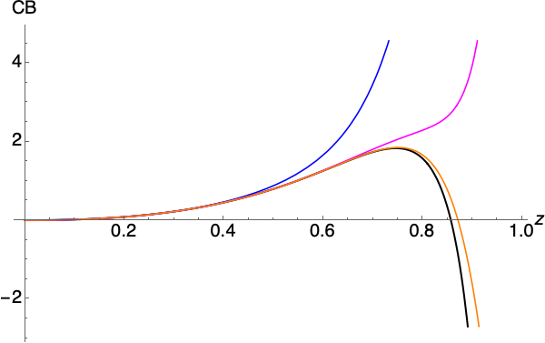
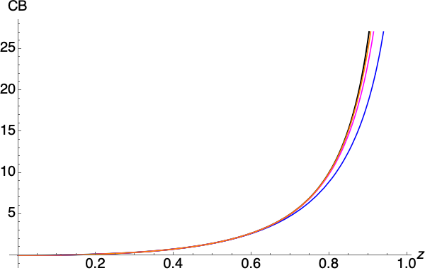
(a) d=2d=2 and (Δ,J)=(2.1,3)(\Delta,J)=(2.1,3) (b) d=4d=4 and (Δ,J)=(2.1,2)(\Delta,J)=(2.1,2)
Figure 1: Numerical match of (2) with known 2 and 4-dimensional conformal blocks in DO-2011 for each (Δ,J)(\Delta,J) and a(s)=b(s)=0{\rm{a}}^{({\rm{s}})}={\rm{b}}^{({\rm{s}})}=0. We have also set z=z¯z=\bar{z} in the horizontal axis. The black curves correspond to the conformal blocks in DO-2011 and the blue, pink and orange curves correspond to the conformal block expansions given in (2) which are truncated at ns=2n_{s}=2, 44 and 66 respectively. We can see that as we increase the number of terms in the summation for Appell’s 𝐅4{\bf{F}}_{4} function, our result quickly approaches the known existing results given by the black curves.

By comparing (2) with (2), we can also regard conformal block with integer spin JJ as the partition summation of scalar conformal blocks with shifted external scaling dimensions:

GΔ,J(s)​(z,z¯)=𝐜Δ,0(s)𝐜Δ,J(s)​∑r,k~​∏i=14Γ⁡(γi(s)​(τ))Γ⁡(γi(s)​(τ)−J+r+∑jki​j)​1uJ−2​r2​GΔ,0(s)​(z,z¯)∣Δi→Δi+∑jki​j.G^{({\rm{s}})}_{\Delta,J}(z,\bar{z})=\frac{{\bf{c}}_{\Delta,0}^{({\rm{s}})}}{{\bf{c}}_{\Delta,J}^{({\rm{s}})}}\widetilde{\sum_{r,k}}\prod_{i=1}^{4}\frac{\Gamma\left(\gamma_{i}^{({\rm{s}})}(\tau)\right)}{\Gamma\left(\gamma_{i}^{({\rm{s}})}(\tau)-J+r+\sum_{j}k_{ij}\right)}\frac{1}{{\rm{u}}^{\frac{J-2r}{2}}}G_{\Delta,0}^{({\rm{s}})}(z,\bar{z})\mid_{\Delta_{i}\to\Delta_{i}+\sum_{j}k_{ij}}. (36)

This is consistent with the observation made in GWD1 (see (5.37) there), where the authors considered the holographic dual configuration to a d-dimensional conformal partial wave, namely “geodesic Witten diagram”, and pointed out a simple relation between the scalar and general tensor exchange cases. Essentially the Gegenbauer polynomial arising from the restriction of spin JJ propagator along the geodesics can only depend on the external coordinates {xi​j2}\{x_{ij}^{2}\} and geodesic parameters. After the integration along the geodesic parameters, the functional form of individual terms in the integrand does not change, only the external scaling dimensions are shifted by integer units which are determined by the multinomial expansion.

We should stress here that an explicit expression for general dd-dimensional conformal block with integer spin JJ was already available in terms of a double infinite series expansion of Gegenbauer polynomials DO-2003 (See also Schomerus1 for the connection with Harish-Chandra functions of B​C2BC_{2} Calogero-Sutherland system), where the expansion coefficients can be determined recursively through the quadratic Casimir equation. Our result (2) provides an alternative explicit expression in terms of a finite summation over Appell’s hypergeometric functions 𝐅4{\bf{F}}_{4} which will facilitate the crossing kernel computation through its Mellin-Barnes representation (28) later. It would be highly non-trivial to demonstrate the equivalence of the two expressions, to this end we can first consider the following non-trivial identity between 𝐅4{{\bf{F}}}_{4} functions and the so-called zonal generalization of hypergeometric function Koornwinder-1:

F12​[a,bc;[z,00,z¯]]=\displaystyle{}_{2}{{F}}_{1}\left[\begin{matrix}~a,~b\\ ~c\end{matrix};\left[\begin{matrix}~z,~0\\ ~0,~\bar{z}\end{matrix}\right]\right]=
Γ⁡(c)Γ⁡(32−c)​Γ​(a)​Γ​(b)​Γ​(c−a)​Γ​(c−b)​(𝐅~4​[a,bc−12,1+a+b−c;u,v]+vc−a−b​𝐅~4​[c−a,c−bc−12,1−a−b+c;u,v]),\displaystyle\small{\frac{\Gamma(c)}{\Gamma(\frac{3}{2}-c)\Gamma(a)\Gamma(b)\Gamma(c-a)\Gamma(c-b)}\left(\tilde{\bf{F}}_{4}\left[\begin{matrix}~a,~b\\ ~c-\frac{1}{2},~1+a+b-c\end{matrix};{\rm{u}},{\rm{v}}\right]+{\rm{v}}^{c-a-b}\tilde{\bf{F}}_{4}\left[\begin{matrix}~c-a,~c-b\\ ~c-\frac{1}{2},~1-a-b+c\end{matrix};{\rm{u}},{\rm{v}}\right]\right)},

where (u,v)({\rm{u}},{\rm{v}}) and (z,z¯)(z,\bar{z}) are related as in (3) and the two variable zonal generalization of F12{}_{2}F_{1} is explicitly given in terms of the Legendre polynomial Pn​(x)P_{n}(x):

F12​[a,bc;[z,00,z¯]]=∑m=0∞∑l=0m(a)m​(a−12)l​(b)m​(b−12)l​(32)m−ll!​(c)m​(c−12)l​(32)m​(12)m−l​um+l2​Pm−l​(σ).{}_{2}{{F}}_{1}\left[\begin{matrix}~a,~b\\ ~c\end{matrix};\left[\begin{matrix}~z,~0\\ ~0,~\bar{z}\end{matrix}\right]\right]=\sum_{m=0}^{\infty}\sum_{l=0}^{m}\frac{(a)_{m}(a-\frac{1}{2})_{l}(b)_{m}(b-\frac{1}{2})_{l}(\frac{3}{2})_{m-l}}{l!(c)_{m}(c-\frac{1}{2})_{l}(\frac{3}{2})_{m}(\frac{1}{2})_{m-l}}{\rm{u}}^{\frac{m+l}{2}}P_{m-l}\left(\sigma\right). (38)

This implies that in our case if we set d=3d=3, a=κσs2​(s)+ra=\kappa_{\sigma_{s}}^{2({\rm{s}})}+r, b=κσs3​(s)+rb=\kappa_{\sigma_{s}}^{3({\rm{s}})}+r and c=32+i​σs​νc=\frac{3}{2}+i\sigma_{s}\nu, we can express the three dimensional scalar conformal partial waves in terms of an infinite summation over Legendre polynomials. More explicitly we have:

GΔ,J(s)​(z,z¯)=1𝐜Δ,J(s)​∑r,k~​∏i=14Γ⁡(κ+i⁡(s)​(τ)+r)Γ⁡(γi(s)​(τ)−J+r+∑jkj​i)​uΔ−J2+r​vk23​∑m=0∞∑l=0m(−1)l\displaystyle G^{({\rm{s}})}_{\Delta,J}(z,\bar{z})=\frac{1}{{\bf{c}}^{({\rm{s}})}_{\Delta,J}}\widetilde{\sum_{r,k}}\prod_{i=1}^{4}\frac{\Gamma\left(\kappa^{i({\rm{s}})}_{+}(\tau)+r\right)}{\Gamma\left(\gamma^{({\rm{s}})}_{i}(\tau)-J+r+\sum_{j}k_{ji}\right)}{\rm{u}}^{\frac{\Delta-J}{2}+r}{\rm{v}}^{k_{23}}\sum_{m=0}^{\infty}\sum_{l=0}^{m}(-1)^{l}
×(32+m)−l​Γ​(h−Δ−l)l!​(12)m−l​(κ+2​(s)​(τ)+r,κ+3​(s)​(τ)+r)m​(κ+2​(s)​(τ)+r−12,κ+3​(s)​(τ)+r−12)lΓ⁡(Δ+m)​um+l2​Cm−l(12)​(σ),\displaystyle\times\frac{(\frac{3}{2}+m)_{-l}\Gamma(h-\Delta-l)}{l!(\frac{1}{2})_{m-l}}\frac{(\kappa_{+}^{2({\rm{s}})}(\tau)+r,\kappa_{+}^{3({\rm{s}})}(\tau)+r)_{m}(\kappa_{+}^{2({\rm{s}})}(\tau)+r-\frac{1}{2},\kappa_{+}^{3({\rm{s}})}(\tau)+r-\frac{1}{2})_{l}}{\Gamma(\Delta+m)}{\rm{u}}^{\frac{m+l}{2}}C_{m-l}^{(\frac{1}{2})}\left(\sigma\right),

and notice that we have used the fact Cn(12)​(σ)=Pn​(σ)C_{n}^{(\frac{1}{2})}(\sigma)=P_{n}(\sigma) for h=32h=\frac{3}{2}. It would be interesting to perform the explicit summation over {r,ki​j}\{r,k_{ij}\} to demonstrate their equivalence. Finally, it is useful to note that at the so-called crossing symmetric point z=z¯=12z=\bar{z}=\frac{1}{2} or u=v=14{\rm{u}}={\rm{v}}=\frac{1}{4} which is popular in conformal bootstrap computations, we can reduce to a generalized hypergeometric function:

𝐅4​[a1,a2c1,c2;u,u]=F34​[a1,a2,c1+c2−12,c1+c22c1,c2,c1+c2−1;4​u],{\bf{F}}_{4}\left[\begin{matrix}~a_{1},~a_{2}\\ ~c_{1},~c_{2}\end{matrix};{\rm{u}},{\rm{u}}\right]={}_{4}F_{3}\left[\begin{matrix}~a_{1},~a_{2},~\frac{c_{1}+c_{2}-1}{2},~\frac{c_{1}+c_{2}}{2}\\ ~c_{1},~c_{2},~c_{1}+c_{2}-1\end{matrix};4{\rm{u}}\right], (40)

this is much easier to be implemented numerically than the 𝐅4{\bf{F}}_{4} function.

Starting with the ss-channel conformal partial wave, we can obtain other equivalent tt- and uu- exchange channels by performing the crossing transformations:

s↔t:(x2,Δ2)↔(x4,Δ4),s↔u:(x2,Δ2)↔(x3,Δ3),{\rm{s}}\leftrightarrow{\rm{t}}~:~(x_{2},\Delta_{2})\leftrightarrow(x_{4},\Delta_{4}),\quad{\rm{s}}\leftrightarrow{\rm{u}}~:~(x_{2},\Delta_{2})\leftrightarrow(x_{3},\Delta_{3}), (41)

or in terms of the conformally invariant cross ratios (3), the crossing transformations act on them as:

s↔t:(u,v)→(v,u);(z,z¯)→(1−z,1−z¯),s↔u:(u,v)→(1/u,v/u);(z,z¯)→(1/z,1/z¯).{\rm{s}}\leftrightarrow{\rm{t}}~:~({\rm{u}},{\rm{v}})\to({\rm{v}},{\rm{u}});~(z,\bar{z})\to(1-z,1-\bar{z}),\quad{\rm{s}}\leftrightarrow{\rm{u}}~:~({\rm{u}},{\rm{v}})\to({1}/{{\rm{u}}},{{\rm{v}}}/{{\rm{u}}});~(z,\bar{z})\to({1}/{z},{1}/{\bar{z}}). (42)

By performing the crossing transformations (3), we can write down the corresponding conformal partial waves in the tt- and uu-channels:

Ψν,J(t)​(xi)\displaystyle\Psi^{({\rm{t}})}_{\nu,J}(x_{i}) =\displaystyle= 𝒯Δi(t)(xi)∑σt=±∑r,k~∏i=141Γ⁡(γi(t)−J+r+∑jkj​i)vτσt+rua(t)+b(t)−k12−k342\displaystyle{\mathcal{T}}^{({\rm{t}})}_{\Delta_{i}}(x_{i})\sum_{\sigma_{t}=\pm}\widetilde{\sum_{r,k}}\prod_{i=1}^{4}\frac{1}{\Gamma\left(\gamma^{({\rm{t}})}_{i}-J+r+\sum_{j}k_{ji}\right)}\frac{{\rm{v}}^{\tau_{\sigma_{t}}+r}}{{\rm{u}}^{\frac{{\rm{a}}^{({\rm{t}})}+{\rm{b}}^{({\rm{t}})}-k_{12}-k_{34}}{2}}}
×\displaystyle\times [uϖ12(t)2​𝐅~4​[κσt1​(t)+r,κσt2​(t)+r1+i​σt​ν,1+ϖ12(t);v,u]+uϖ34(t)2​𝐅~4​[κσt3​(t)+r,κσt4​(t)+r1+i​σt​ν,1+ϖ34(t);v,u]],\displaystyle{\left[{\rm{u}}^{\frac{\varpi_{12}^{({\rm{t}})}}{2}}\tilde{\bf{F}}_{4}\left[\begin{matrix}~\kappa_{\sigma_{t}}^{1({\rm{t}})}+r,~\kappa_{\sigma_{t}}^{2({\rm{t}})}+r\\ ~1+i\sigma_{t}\nu,~1+\varpi_{12}^{({\rm{t}})}\end{matrix};{\rm{v}},{\rm{u}}\right]+{\rm{u}}^{\frac{\varpi^{({\rm{t}})}_{34}}{2}}\tilde{\bf{F}}_{4}\left[\begin{matrix}~\kappa_{\sigma_{t}}^{3({\rm{t}})}+r,~\kappa_{\sigma_{t}}^{4({\rm{t}})}+r\\ ~1+i\sigma_{t}\nu,~1+\varpi_{34}^{({\rm{t}})}\end{matrix};{\rm{v}},{\rm{u}}\right]\right]},
Ψν,J(u)​(xi)\displaystyle\Psi^{({\rm{u}})}_{\nu,J}(x_{i}) =\displaystyle= 𝒯Δi(u)(xi)∑σu=±∑r,k~∏i=141Γ⁡(γi(u)−J+r+∑jkj​i)(1u)τσu+r(vu)a(u)+b(u)−k14−k232\displaystyle{\mathcal{T}}^{({\rm{u}})}_{\Delta_{i}}(x_{i})\sum_{\sigma_{u}=\pm}\widetilde{\sum_{r,k}}\prod_{i=1}^{4}\frac{1}{\Gamma\left(\gamma^{({\rm{u}})}_{i}-J+r+\sum_{j}k_{ji}\right)}\frac{(\frac{1}{{\rm{u}}})^{\tau_{\sigma_{u}}+r}}{(\frac{{\rm{v}}}{{\rm{u}}})^{\frac{{\rm{a}}^{({\rm{u}})}+{\rm{b}}^{({\rm{u}})}-k_{14}-k_{23}}{2}}}
×\displaystyle\times [(vu)ϖ14(u)2​𝐅~4​[κσu1​(u)+r,κσu4​(u)+r1+i​σu​ν,1+ϖ14(u);1u,vu]+(vu)ϖ23(u)2​𝐅~4​[κσu2​(u)+r,κσu3​(u)+r1+i​σu​ν,1+ϖ23(u);1u,vu]].\displaystyle{\left[\left(\frac{{\rm{v}}}{{\rm{u}}}\right)^{\frac{\varpi_{14}^{({\rm{u}})}}{2}}\tilde{\bf{F}}_{4}\left[\begin{matrix}~\kappa_{\sigma_{u}}^{1({\rm{u}})}+r,~\kappa_{\sigma_{u}}^{4({\rm{u}})}+r\\ ~1+i\sigma_{u}\nu,~1+\varpi^{({\rm{u}})}_{14}\end{matrix};\frac{1}{{\rm{u}}},\frac{{\rm{v}}}{{\rm{u}}}\right]+\left(\frac{{\rm{v}}}{{\rm{u}}}\right)^{\frac{\varpi_{23}^{({\rm{u}})}}{2}}\tilde{\bf{F}}_{4}\left[\begin{matrix}~\kappa_{\sigma_{u}}^{2({\rm{u}})}+r,~\kappa_{\sigma_{u}}^{3({\rm{u}})}+r\\ ~1+i\sigma_{u}\nu,~1+\varpi_{23}^{({\rm{u}})}\end{matrix};\frac{1}{{\rm{u}}},\frac{{\rm{v}}}{{\rm{u}}}\right]\right]}.

Here we have used the crossing transformations (42) to change the cross ratios, while various remaining parameters (κσti⁡(t),γi(t),κσui⁡(u),γi(u))(\kappa_{\sigma_{t}}^{i({\rm{t}})},\gamma_{i}^{({\rm{t}})};\kappa_{\sigma_{u}}^{i({\rm{u}})},\gamma_{i}^{({\rm{u}})}) and pre-factors (𝒯Δi(t)​(xi),𝒯Δi(u)​(xi))({\mathcal{T}}^{({\rm{t}})}_{\Delta_{i}}(x_{i}),{\mathcal{T}}^{({\rm{u}})}_{\Delta_{i}}(x_{i})) can be obtained from (22) and (2) using the crossing transformations (41). It is interesting to note that the ss and tt-channel conformal partial waves are both convergent within the square given by 0<u,v<10<{\rm{u}},{\rm{v}}<1 or equivalently 0<z,z¯<10<z,\bar{z}<1, this becomes important when we compute the crossing kernel, as we need to use the expressions for the integrand which are convergent in a given integration region.

3 Generalization to Continuous Spins

For our computation of the crossing kernel using the inversion formula of CH-2017 in the next section, here we would also like to consider the scalar conformal block in arbitrary dimensions with continuous spin JJ by generalizing our earlier construction. Recall that the Mellin representation for conformal partial wave with integer JJ (16) can be derived from pairing two copies of three point functions related through a shadow transformation and the contraction of their symmetric traceless tensor structures yields a Gegenbauer polynomial CJ(ε)​(η)C_{J}^{(\varepsilon)}(\eta) in the process, see for example DO-2011, CKK2. Now for continuous spin JJ, we need to generalize the shadow to “full-shadow” transformation LightRay, this involves contracting two copies of three point functions whose spins are also related via the spin shadow transformation Work1. The net result here is to replace the Gegenbauer polynomial arising from the contraction of two symmetric traceless tensors with identical integer spin JJ:

X^{μ1…X^μJ}Y^{μ1…Y^μJ}=12J​cJF12[−J,J+2​εε+12;1−η2]=12J​cJC^J(ε)(η),η=X^⋅Y^\hat{X}^{\{\mu_{1}\dots}\hat{X}^{\mu_{J}\}}\hat{Y}_{\{\mu_{1}\dots}\hat{Y}_{\mu_{J}\}}=\frac{1}{2^{J}c_{J}}{}_{2}F_{1}\left[\begin{matrix}~-J,~J+2\varepsilon\\ \varepsilon+\frac{1}{2}\end{matrix};\frac{1-\eta}{2}\right]=\frac{1}{2^{J}c_{J}}\hat{C}_{J}^{(\varepsilon)}(\eta),~~\eta={\hat{X}\cdot\hat{Y}} (45)

where X^,Y^\hat{X},\hat{Y} are unit vectors and C^J(ε)​(η)=J!(2​ε)J​CJ(ε)​(η)\hat{C}_{J}^{(\varepsilon)}(\eta)=\frac{J!}{(2\varepsilon)_{J}}C_{J}^{(\varepsilon)}(\eta), by its continuous spin generalization through integration over the null polarization vector zνz^{\nu} LightRay:

∫D2​εz(−2z⋅X^)J(−2z⋅Y^)J¯=πεΓ⁡(ε)Γ⁡(2​ε)F12[−J,−J¯ε+12;1−η2],\displaystyle\int D^{2\varepsilon}z(-2z\cdot\hat{X})^{J}(-2z\cdot\hat{Y})^{\bar{J}}=\pi^{\varepsilon}\frac{\Gamma(\varepsilon)}{\Gamma(2\varepsilon)}{}_{2}F_{1}\left[\begin{matrix}~-J,~-\bar{J}\\ \varepsilon+\frac{1}{2}\end{matrix};\frac{1-\eta}{2}\right],
=πε​{Γ⁡(J+ε)Γ⁡(J+2​ε)​(2​η)J​F12​[−J2,1−J22−h−J;1η2]+Γ⁡(J¯+ε)Γ⁡(J¯+2​ε)​(2​η)J¯​F12​[−J¯2,1−J¯22−h−J¯;1η2]}.\displaystyle=\pi^{\varepsilon}\left\{\frac{\Gamma(J+\varepsilon)}{\Gamma(J+2\varepsilon)}(2\eta)^{J}{}_{2}F_{1}\left[\begin{matrix}~-\frac{J}{2},~\frac{1-J}{2}\\ 2-h-J\end{matrix};\frac{1}{\eta^{2}}\right]+\frac{\Gamma(\bar{J}+\varepsilon)}{\Gamma(\bar{J}+2\varepsilon)}(2\eta)^{\bar{J}}{}_{2}F_{1}\left[\begin{matrix}~-\frac{\bar{J}}{2},~\frac{1-\bar{J}}{2}\\ 2-h-\bar{J}\end{matrix};\frac{1}{\eta^{2}}\right]\right\}.

Here we have introduced the shadow spin J¯=−2​ε−J\bar{J}=-2\varepsilon-J and the scale-invariant integration measure over polarization vector zμz^{\mu}:

D2​ε​z≡dd​z​θ​(z0)​δ​(z2)vol​ℝ+.D^{2\varepsilon}z\equiv\frac{d^{d}z\theta(z^{0})\delta(z^{2})}{{\rm vol}{\mathbb{R}}_{+}}. (47)

where the division by the volume of the group of positive rescaling vol​ℝ+{{\rm vol}{\mathbb{R}}_{+}} ensures the finite result. In the second equality of (3), we have separated the dependence on continuous spin JJ and its shadow J¯\bar{J} using hypergeometric identity. It is clear that unless in even dimensions, i.e. ε=0,1,2,…\varepsilon=0,1,2,\dots etc., the Γ\Gamma-functions in the pre-factors ensure that when J∈ℤ≥0J\in{\mathbb{Z}}_{\geq 0} or equivalently J¯+2​ε∈ℤ≤0\bar{J}+2\varepsilon\in{\mathbb{Z}}_{\leq 0}, the J¯\bar{J}-dependent term vanishes identically and vice versa.

The rest of the computation proceeds almost identically as in the integer spin case, the Mellin representation for the conformal partial wave with continuous spin is now given by two distinct spin-dependent parts:

Ψ~ν,ℓ(s)​(xi)\displaystyle\tilde{\Psi}_{\nu,\ell}^{({\rm{s}})}(x_{i}) =\displaystyle= 𝒯Δi(s)​(xi)​∫−i​∞i​∞d​s(4​π​i)​∫−i​∞i​∞d​t(4​π​i)​us2​vt2​ρΔi(s)​(s,t)​(Γ⁡(+i​ℓ)Γ⁡(ε+i​ℓ)​𝐌ν,+ℓ(s)​(s,t)+Γ⁡(−i​ℓ)Γ⁡(ε−i​ℓ)​𝐌ν,−ℓ(s)​(s,t))\displaystyle{\mathcal{T}}_{\Delta_{i}}^{({\rm{s}})}(x_{i})\int^{i\infty}_{-i\infty}\frac{ds}{(4\pi i)}\int^{i\infty}_{-i\infty}\frac{dt}{(4\pi i)}{\rm{u}}^{\frac{s}{2}}{\rm{v}}^{\frac{t}{2}}\rho^{({\rm{s}})}_{\Delta_{i}}(s,t)\left(\frac{\Gamma(+i\ell)}{\Gamma(\varepsilon+i\ell)}{\bf{M}}^{({\rm{s}})}_{\nu,+\ell}(s,t)+\frac{\Gamma(-i\ell)}{\Gamma(\varepsilon-i\ell)}{\bf{M}}^{({\rm{s}})}_{\nu,-\ell}(s,t)\right) (48)
=\displaystyle= 𝒯Δi(s)(xi)∑σs=±∑ηs=±𝐜^h+i​σs​ν,−ε+i​ηs​ℓΓ⁡(i​ηs​ℓ)Γ⁡(ε+i​ηs​ℓ)𝔤h+i​σs​ν,−ε+i​ηs​ℓ(s)(z,z¯).\displaystyle{\mathcal{T}}_{\Delta_{i}}^{({\rm{s}})}(x_{i})\sum_{\sigma_{s}=\pm}\sum_{\eta_{s}=\pm}\hat{{\bf{c}}}_{h+i\sigma_{s}\nu,-\varepsilon+i\eta_{s}\ell}\frac{\Gamma(i\eta_{s}\ell)}{\Gamma(\varepsilon+i\eta_{s}\ell)}{\mathfrak{g}}_{h+i\sigma_{s}\nu,-\varepsilon+i\eta_{s}\ell}^{({\rm{s}})}(z,\bar{z}).

Here we have also parameterized continuous spin J=−ε+i​ℓJ=-\varepsilon+i\ell and shadow spin J¯=−ε−i​ℓ\bar{J}=-\varepsilon-i\ell through spectral parameter ℓ\ell, putting it on equal footing as the scaling dimension. In the last line of (48), we have made both shadow and spin-shadow transformations manifest after (s,t)(s,t)-integration by expressing them in terms of the building blocks 𝔤h+i​σs​ν,−ε+i​ηs​ℓ(s)​(z,z¯){\mathfrak{g}}_{h+i\sigma_{s}\nu,-\varepsilon+i\eta_{s}\ell}^{({\rm{s}})}(z,\bar{z}) whose explicit form will be given momentarily. Here the normalization constants:

𝐜^h+i​σs​ν,−ε+i​ηs​ℓ=2−ε+i​ηs​ℓ​πε​Γ⁡(−i​σs​ν)​Γ​(−i​σs​ν+i​ηs​ℓ)Γ⁡(2​ωσs​ηs)​Γ​(h−i​σs​ν−1)​Γ⁡(ωσs​ηs±a(s))​Γ​(ωσs​ηs±b(s))∏i=14Γ⁡(γi​ηs(s)).\hat{{\bf{c}}}_{h+i\sigma_{s}\nu,-\varepsilon+i\eta_{s}\ell}={2^{-\varepsilon+i\eta_{s}\ell}}\pi^{\varepsilon}\frac{\Gamma(-i\sigma_{s}\nu)\Gamma(-i\sigma_{s}\nu+i\eta_{s}\ell)}{\Gamma(2\omega_{\sigma_{s}\eta_{s}})\Gamma(h-i\sigma_{s}\nu-1)}\frac{\Gamma\left(\omega_{\sigma_{s}\eta_{s}}\pm{\rm{a}}^{({\rm{s}})}\right)\Gamma\left(\omega_{\sigma_{s}\eta_{s}}\pm{\rm{b}}^{({\rm{s}})}\right)}{\prod_{i=1}^{4}\Gamma\left(\gamma_{i\eta_{s}}^{({\rm{s}})}\right)}. (49)

are fixed by comparing (3) with (45) and (2), such that JJ becomes an non-negative integer, we recover the conformal block given in (2) from 𝔤Δ,J(s)​(z,z¯){\mathfrak{g}}_{\Delta,J}^{({\rm{s}})}(z,\bar{z}). We can also define the following parameters:

τσs​ηs=h+i​σs​ν−(−ε+i​ηs​ℓ)2,ωσs​ηs=h+i​σs​ν+(−ε+i​ηs​ℓ)2,σs,ηs=±,\tau_{\sigma_{s}\eta_{s}}=\frac{h+i\sigma_{s}\nu-(-\varepsilon+i\eta_{s}\ell)}{2},\quad\omega_{\sigma_{s}\eta_{s}}=\frac{h+i\sigma_{s}\nu+(-\varepsilon+i\eta_{s}\ell)}{2},\quad\sigma_{s},\eta_{s}=\pm, (50)
γ1​ηs(s)=ω+ηs−a(s),γ2​ηs(s)=ω+ηs+a(s),γ3​ηs(s)=ω−ηs+b(s),γ4​ηs(s)=ω−ηs−b(s).\gamma_{1\eta_{s}}^{({\rm{s}})}=\omega_{+\eta_{s}}-{\rm{a}}^{({\rm{s}})},~\gamma_{2\eta_{s}}^{({\rm{s}})}=\omega_{+\eta_{s}}+{\rm{a}}^{({\rm{s}})},~\gamma_{3\eta_{s}}^{({\rm{s}})}=\omega_{-\eta_{s}}+{\rm{b}}^{({\rm{s}})},~\gamma_{4\eta_{s}}^{({\rm{s}})}=\omega_{-\eta_{s}}-{\rm{b}}^{({\rm{s}})}. (51)
κσs​ηs1​(s)=τσs​ηs−a(s)+k13+k14,κσs​ηs2​(s)=τσs​ηs+a(s)+k23+k24,\displaystyle\kappa_{\sigma_{s}\eta_{s}}^{1({\rm{s}})}=\tau_{\sigma_{s}\eta_{s}}-{\rm{a}}^{({\rm{s}})}+k_{13}+k_{14},~\kappa_{\sigma_{s}\eta_{s}}^{2({\rm{s}})}=\tau_{\sigma_{s}\eta_{s}}+{\rm{a}}^{({\rm{s}})}+k_{23}+k_{24},
κσs​ηs3​(s)=τσs​ηs+b(s)+k13+k23,κσs​ηs4​(s)=τσs​ηs−b(s)+k14+k24.\displaystyle\kappa_{\sigma_{s}\eta_{s}}^{3({\rm{s}})}=\tau_{\sigma_{s}\eta_{s}}+{\rm{b}}^{({\rm{s}})}+k_{13}+k_{23},~\kappa_{\sigma_{s}\eta_{s}}^{4({\rm{s}})}=\tau_{\sigma_{s}\eta_{s}}-{\rm{b}}^{({\rm{s}})}+k_{14}+k_{24}. (52)

and the precise definition of non-integral summation indices {ki​j}\{k_{ij}\} is given around (56). We can now write down 𝐌ν,ηs​ℓ(s)​(s,t){\bf{M}}^{({\rm{s}})}_{\nu,\eta_{s}\ell}(s,t), each contains two pieces related by shadow transformation after the Mellin variable (s,t)(s,t) integrations:

𝐌ν,ηs​ℓ(s)​(s,t)=πε∏i=14Γ⁡(γi​ηs(s))​Γ⁡(τ±ηs−s2)Γ⁡(δ12(s))​Γ​(δ34(s))​Q~ν,ηs​ℓ(s)​(s,t),\displaystyle{\bf{M}}^{({\rm{s}})}_{\nu,\eta_{s}\ell}(s,t)=\frac{\pi^{\varepsilon}}{\prod_{i=1}^{4}\Gamma\left(\gamma_{i\eta_{s}}^{({\rm{s}})}\right)}\frac{\Gamma\left(\tau_{\pm\eta_{s}}-\frac{s}{2}\right)}{\Gamma(\delta_{12}^{({\rm{s}})})\Gamma(\delta_{34}^{({\rm{s}})})}\tilde{Q}_{\nu,\eta_{s}\ell}^{({\rm{s}})}(s,t), (53)
Q~ν,ηs​ℓ(s)​(s,t)=∑m,k~​(τ±ηs−s2)m​∏(i​j)Γ⁡(δi​j(s)+ki​j)Γ⁡(δi​j(s))​∏i=14Γ⁡(γi​η(s))Γ⁡(γi​ηs(s)−(−ε+i​ηs​ℓ)+m+∑jki​j).\displaystyle\tilde{Q}_{\nu,\eta_{s}\ell}^{({\rm{s}})}(s,t)=\widetilde{\sum_{m,k}}\left(\tau_{\pm\eta_{s}}-\frac{s}{2}\right)_{m}\prod_{(ij)}\frac{\Gamma\left(\delta_{ij}^{({\rm{s}})}+k_{ij}\right)}{\Gamma\left(\delta_{ij}^{({\rm{s}})}\right)}\prod_{i=1}^{4}\frac{\Gamma\left(\gamma_{i\eta}^{({\rm{s}})}\right)}{\Gamma\left(\gamma_{i\eta_{s}}^{({\rm{s}})}-(-\varepsilon+i\eta_{s}\ell)+m+\sum_{j}k_{ij}\right)}.

We can regard Q~ν,η​ℓ(s)​(s,t)\tilde{Q}_{\nu,\eta\ell}^{({\rm{s}})}(s,t) as a continuous spin generalization of a Mack polynomial, here {δi​j(s)}\{\delta_{ij}^{({\rm{s}})}\} containing Mellin variables are parameterized as before (18). The abridged infinite summation is given by :

∑m,k~​⋯≡∑m=0∞22​m​(ε−i​ηs​ℓ2)m​(h−i​ηs​ℓ2)mm!​(1−i​ηs​ℓ)m​∑∑ki​j=−ε+i​ηs​ℓ−2​m~​(−1)k13+k24​Γ⁡(−ε+i​ηs​ℓ−2​m+1)∏(i​j)Γ⁡(ki​j+1)​…,\widetilde{\sum_{m,k}}\dots\equiv\sum_{m=0}^{\infty}2^{2m}\frac{(\frac{\varepsilon-i\eta_{s}\ell}{2})_{m}(\frac{h-i\eta_{s}\ell}{2})_{m}}{m!(1-i\eta_{s}\ell)_{m}}\widetilde{\sum_{\sum k_{ij}=-\varepsilon+i\eta_{s}\ell-2m}}(-1)^{k_{13}+k_{24}}\frac{\Gamma(-\varepsilon+i\eta_{s}\ell-2m+1)}{\prod_{(ij)}\Gamma(k_{ij}+1)}\dots, (55)

where the first infinite summation over mm comes from the expansion of a F12{}_{2}F_{1} function, while the remaining summation comes from analytically continuing the multinomial theorem to continuous power Hilliker, such that it is also an infinite summation:

∑∑ki​j​⋯=−ε+i​ηs​ℓ−2​m~≡∑p=0∞∑k14+k24+k13=p…,k24=−ε+i​ηs​ℓ−2​m−p.\widetilde{\sum_{\sum k_{ij}\dots=-\varepsilon+i\eta_{s}\ell-2m}}\equiv\sum_{p=0}^{\infty}\sum_{k_{14}+k_{24}+k_{13}=p}\dots,~~k_{24}=-\varepsilon+i\eta_{s}\ell-2m-p. (56)

In other words, we generalize the earlier four-fold partition of integer spin by picking one of the four k(i​j)k_{(ij)}, say k24k_{24} to be a continuous parameter. Altogether, as in the integer spin case, we now have five (non-independent) summations, even though the range now expands to infinities to account for continuous spin.

To obtain the conformal block in general dd-dimension with continuous spin GΔ,J(s)​(z,z¯)G_{\Delta,J}^{({\rm{s}})}(z,\bar{z}), we can explicitly integrate over Mellin variables (s,t)(s,t) as before to obtain the building block 𝔤Δ,J(s)​(z,z¯){\mathfrak{g}}_{\Delta,J}^{({\rm{s}})}(z,\bar{z}) and 𝔤Δ,J¯(s)​(z,z¯){\mathfrak{g}}_{\Delta,\bar{J}}^{({\rm{s}})}(z,\bar{z}) in terms of Appell’s hypergeometric function F4F_{4}, as the pole structures remain the same here. We can then consider the following linear combination88 8 Notice that we could have chosen slightly more symmetric combination such as: GΔ,J(s)​(z,z¯)∼Γ⁡(J+ε)Γ⁡(J+2​ε)​𝔤Δ,J(s)​(z,z¯)+Γ⁡(J¯+ε)Γ⁡(J¯+2​ε)​𝔤Δ,J¯(s)​(z,z¯),G_{\Delta,J}^{({\rm{s}})}(z,\bar{z})\sim\frac{\Gamma(J+\varepsilon)}{\Gamma(J+2\varepsilon)}{\mathfrak{g}}_{\Delta,J}^{({\rm{s}})}(z,\bar{z})+\frac{\Gamma(\bar{J}+\varepsilon)}{\Gamma(\bar{J}+2\varepsilon)}{\mathfrak{g}}_{\Delta,\bar{J}}^{({\rm{s}})}(z,\bar{z}), (57) however the normalization of the conformal block will need to change accordingly. :

GΔ,J(s)​(z,z¯)=𝔤Δ,J(s)​(z,z¯)+Γ⁡(J+2​ε)​Γ​(J¯+ε)Γ⁡(J¯+2​ε)​Γ​(J+ε)​𝔤Δ,J¯(s)​(z,z¯),\displaystyle G^{({\rm{s}})}_{\Delta,J}(z,\bar{z})={\mathfrak{g}}_{\Delta,J}^{({\rm{s}})}(z,\bar{z})+\frac{\Gamma(J+2\varepsilon)\Gamma(\bar{J}+\varepsilon)}{\Gamma(\bar{J}+2\varepsilon)\Gamma(J+\varepsilon)}{\mathfrak{g}}_{\Delta,\bar{J}}^{({\rm{s}})}(z,\bar{z}), (58)

where the building blocks are given explicitly by

𝔤Δ,J(s)​(z,z¯)=πε𝐜^Δ,J​∑m,k~​∏i=141Γ⁡(γi+(s)​(Δ,J)−J+m+∑jki​j)​uΔ−J2+mva(s)+b(s)−k14−k232\displaystyle{\mathfrak{g}}_{\Delta,J}^{({\rm{s}})}(z,\bar{z})=\frac{\pi^{\varepsilon}}{\hat{{\bf{c}}}_{\Delta,J}}\widetilde{\sum_{m,k}}\prod_{i=1}^{4}\frac{1}{\Gamma\left(\gamma_{i+}^{({\rm{s}})}(\Delta,J)-J+m+\sum_{j}k_{ij}\right)}\frac{{\rm{u}}^{\frac{\Delta-J}{2}+m}}{{\rm{v}}^{\frac{{\rm{a}}^{({\rm{s}})}+{\rm{b}}^{({\rm{s}})}-k_{14}-k_{23}}{2}}}
×[vϖ14(s)2​𝐅~4​[κ+⁣+1​(s)​(Δ,J)+m,κ+⁣+4​(s)​(Δ,J)+m1−h+Δ,1+ϖ14(s);u,v]+vϖ23(s)2​𝐅~4​[κ+⁣+2​(s)​(Δ,J)+m,κ+⁣+3​(s)​(Δ,J)+m1−h+Δ,1+ϖ23(s);u,v]],\displaystyle\times{\left[{\rm{v}}^{\frac{\varpi_{14}^{({\rm{s}})}}{2}}\tilde{\bf{F}}_{4}\left[\begin{matrix}~\kappa_{++}^{1({\rm{s}})}(\Delta,J)+m,~\kappa_{++}^{4({\rm{s}})}(\Delta,J)+m\\ ~1-h+\Delta,~1+\varpi_{14}^{({\rm{s}})}\end{matrix};{\rm{u}},{\rm{v}}\right]+{\rm{v}}^{\frac{\varpi_{23}^{({\rm{s}})}}{2}}\tilde{\bf{F}}_{4}\left[\begin{matrix}~\kappa_{++}^{2({\rm{s}})}(\Delta,J)+m,~\kappa_{++}^{3({\rm{s}})}(\Delta,J)+m\\ ~1-h+\Delta,~1+\varpi_{23}^{({\rm{s}})}\end{matrix};{\rm{u}},{\rm{v}}\right]\right]},

while ϖ14(s)\varpi_{14}^{({\rm{s}})} and ϖ23(s)\varpi_{23}^{({\rm{s}})} remain the same in (25) and (26). Here γi+(s)​(Δ,J)\gamma_{i+}^{({\rm{s}})}(\Delta,J) and κ+⁣+i⁡(s)​(Δ,J)\kappa_{++}^{i({\rm{s}})}(\Delta,J) are given by setting h+i​ν=Δh+i\nu=\Delta and −ε+i​ℓ=J-\varepsilon+i\ell=J in γi+(s)\gamma_{i+}^{({\rm{s}})} and κ+⁣+i⁡(s)\kappa_{++}^{i({\rm{s}})} defined in (51) and (3), while 𝔤Δ,J¯(s)​(z,z¯){\mathfrak{g}}_{\Delta,\bar{J}}^{({\rm{s}})}(z,\bar{z}) can be obtained by obvious J→J¯J\to\bar{J} replacements in the parameters, such as setting h+i​ν=Δh+i\nu=\Delta and −ε−i​ℓ=J¯-\varepsilon-i\ell=\bar{J} in γi−(s)\gamma_{i-}^{({\rm{s}})} and κ+⁣−i⁡(s)\kappa_{+-}^{i({\rm{s}})} to obtain γi−(s)​(Δ,J¯)\gamma_{i-}^{({\rm{s}})}(\Delta,\bar{J}) and κ+⁣−i⁡(s)​(Δ,J¯)\kappa_{+-}^{i({\rm{s}})}(\Delta,\bar{J}) respectively. One should keep in mind that one of {k(i​j)}\{k_{(ij)}\} is now a non-integer, we should perform infinite summation as in (56) instead. We have numerically checked that our expression matches with the known results for the conformal blocks with continuous spin in d=2,4d=2,4 dimensions, i.e. directly taking JJ to be continuous in the argument of hypergeometric functions as was done in Liu-2018.

We should note previously the explicit form of scalar conformal block with continuous spin JJ was also constructed in Schomerus1, where the authors constructed the following linear combination:

GΔ,J(s)​IS​(z,z¯)=(ε)J(2​ε)J​Φ^Δ,J(s)​(z,z¯)+(ε)J¯(2​ε)J¯​Φ^Δ,J¯(s)​(z,z¯),Φ^Δ,J(s)​(z,z¯)=24​a(s)+2​Δ(z​z¯)a(s)​Φ~Δ,J(s)​(z,z¯).G_{\Delta,J}^{({\rm{s}}){\rm IS}}(z,\bar{z})=\frac{(\varepsilon)_{J}}{(2\varepsilon)_{J}}\hat{\Phi}_{\Delta,J}^{({\rm{s}})}(z,\bar{z})+\frac{(\varepsilon)_{\bar{J}}}{(2\varepsilon)_{\bar{J}}}\hat{\Phi}_{\Delta,\bar{J}}^{({\rm{s}})}(z,\bar{z}),~~\hat{\Phi}_{\Delta,J}^{({\rm{s}})}(z,\bar{z})=\frac{2^{4{\rm{a}}^{({\rm{s}})}+2\Delta}}{(z\bar{z})^{{\rm{a}}^{({\rm{s}})}}}\tilde{\Phi}_{\Delta,J}^{({\rm{s}})}(z,\bar{z}). (60)

Here Φ~Δ,J(s)​(z,z¯)\tilde{\Phi}_{\Delta,J}^{({\rm{s}})}(z,\bar{z}) is the so-called twisted Harish-Chandra function which is related to the eigenfunction of the B​C2BC_{2} Calogero-Sutherland Hamiltonian via a similarity transformation. The explicit form of Φ~Δ,J(s)​(z,z¯)\tilde{\Phi}_{\Delta,J}^{({\rm{s}})}(z,\bar{z}) depends on (Δ,J,a(s),b(s),h)(\Delta,J,{\rm{a}}^{({\rm{s}})},{\rm{b}}^{({\rm{s}})},h) and can be written in terms of a double infinite series involving F12{}_{2}F_{1}. While in CH-2017, it was proposed that the scalar conformal block with continuous JJ exchange can be decomposed as

GΔ,J(s)​CH​(z,z¯)=gΔ,Jpure​(z,z¯)+Γ⁡(J+2​ε)​Γ​(J¯+ε)Γ⁡(J¯+2​ε)​Γ​(J+ε)​gΔ,J¯pure​(z,z¯),G_{\Delta,J}^{({\rm{s}}){\rm CH}}(z,\bar{z})=g^{\rm pure}_{\Delta,J}(z,\bar{z})+\frac{\Gamma(J+2\varepsilon)\Gamma(\bar{J}+\varepsilon)}{\Gamma(\bar{J}+2\varepsilon)\Gamma(J+\varepsilon)}g^{\rm pure}_{\Delta,\bar{J}}(z,\bar{z}), (61)

where the function gΔ,Jpure​(z,z¯)g_{\Delta,J}^{\rm pure}(z,\bar{z}) in CH-2017, which is also a solution of the quadratic Casimir equation (4), but with different asymptotic behavior from GΔ,J(s)​(z,z¯)G_{\Delta,J}^{({\rm{s}})}(z,\bar{z}), i.e.:

GΔ,J(s)​IS/CH​(z,z¯)\displaystyle G_{\Delta,J}^{({\rm{s}}){\rm IS/CH}}(z,\bar{z}) →\displaystyle\to (Const.)(zz¯)Δ2F12[−J,−J¯ε+12;1−σ2]+𝒪((zz¯)Δ2+1),\displaystyle({\rm{Const.}})(z\bar{z})^{\frac{\Delta}{2}}{}_{2}F_{1}\left[\begin{matrix}~-J,~-\bar{J}\\ \varepsilon+\frac{1}{2}\end{matrix};\frac{1-\sigma}{2}\right]+{\mathcal{O}}\left((z\bar{z})^{\frac{\Delta}{2}+1}\right), (62)
gΔ,Jpure​(z,z¯)\displaystyle g^{\rm pure}_{\Delta,J}(z,\bar{z}) →\displaystyle\to (z​z¯)Δ2​(2​σ)J​F12​[−J2,1−J22−h−J;1σ2]+𝒪⁡((z​z¯)Δ2+1),z​z¯→0,σ=z+z¯2​z​z¯​fixed.\displaystyle(z\bar{z})^{\frac{\Delta}{2}}(2\sigma)^{J}{}_{2}F_{1}\left[\begin{matrix}~-\frac{J}{2},~\frac{1-J}{2}\\ 2-h-J\end{matrix};\frac{1}{\sigma^{2}}\right]+{\mathcal{O}}\left((z\bar{z})^{\frac{\Delta}{2}+1}\right),\quad z\bar{z}\to 0,~\sigma=\frac{z+\bar{z}}{2\sqrt{z\bar{z}}}~~{\rm fixed}.

The two distinct asymptotic behaviors (62) and (3) can be reconciled using the hypergeometric function identity given in (3), this also implies that (60) and (61) can be directly matched if Φ^Δ,J(s)​(z,z¯)\hat{\Phi}_{\Delta,J}^{({\rm{s}})}(z,\bar{z}) and gΔ,Jpure​(z,z¯)g^{\rm pure}_{\Delta,J}(z,\bar{z}) are identified up to an overall constant factor, as it was indeed done in Schomerus1. We have also numerically checked asymptotic behavior of our expression for continuous spin conformal block (58), which also matches with (62) up to an overall constant for continuous (Δ,J)(\Delta,J). This implies that our expression 𝔤Δ,J¯(s)​(z,z¯){\mathfrak{g}}_{\Delta,\bar{J}}^{({\rm{s}})}(z,\bar{z}) (3) provides an alternative expression for the twisted Harish Chandra function Φ^Δ,J¯(s)​(z,z¯)\hat{\Phi}_{\Delta,\bar{J}}^{({\rm{s}})}(z,\bar{z}) hence gΔ,Jpure​(z,z¯)g^{\rm pure}_{\Delta,J}(z,\bar{z}) as derived from the corresponding Mellin amplitude (53) and (3). It would be interesting but non-trivial to analytically demonstrate the full functional equivalence of (3) and Φ^Δ,J¯(s)​(z,z¯)\hat{\Phi}_{\Delta,\bar{J}}^{({\rm{s}})}(z,\bar{z}) using appropriate hypergeometric function identities, while it seems obvious to us they should match, as they both solve the quadratic Casimir equation and their asymptotic behaviors numerically match.

4 Lorentzian Crossing Kernel and Kampé de Fériet Functions

In the Euclidean space ℝd{\mathbb{R}}^{d}, the conformal partial wave Ψν,J(s)​(xi)\Psi_{\nu,J}^{({\rm{s}})}(x_{i}) (23) for integer spin JJ is known to satisfy the orthogonality condition CH-2017; SSW-2017 with respect to the following inner product:

(Ψν,J(s)​(xi),Ψν′,J′(s)​(xi))=∫∏i=14dd​xiVol⁡(S​O​(1,d+1))​Ψν,J(s)​(xi)​Ψ¯ν′,J′(s)​(xi)=2​π​𝒩ν,J​(δ⁡(ν−ν′)+𝒦ν​δ​(ν+ν′))​δJ,J′,\left(\Psi^{({\rm{s}})}_{\nu,J}(x_{i}),{\Psi^{({\rm{s}})}_{\nu^{\prime},J^{\prime}}}(x_{i})\right)=\int\frac{\prod_{i=1}^{4}d^{d}x_{i}}{{\rm Vol}(SO(1,d+1))}\Psi^{({\rm{s}})}_{\nu,J}(x_{i})\overline{\Psi}^{({\rm{s}})}_{\nu^{\prime},J^{\prime}}(x_{i})=2\pi{{\mathcal{N}}_{\nu,J}}\left(\delta(\nu-\nu^{\prime})+{\mathcal{K}}_{\nu}\,\delta(\nu+\nu^{\prime})\right)\delta_{J,J^{\prime}}, (64)

where 𝒩ν,J{\mathcal{N}}_{\nu,J} is the overall normalization factor99 9 Here we take the overall normalization factor to be: 𝒩ν,J=λ02​πd+122​(J+ε)​vol⁡(Sd−2)vol⁡(S​O​(d−1))​(2​J+2​ε)​Γ​(J+1)​Γ​(J+2​ε)Γ​(J+h)2​Γ⁡(±i​ν)Γ⁡(h±i​ν−1)​Γ​(h±i​ν−J−1).{\mathcal{N}}_{\nu,J}=\lambda_{0}^{2}\frac{\pi^{d+1}}{2^{2(J+\varepsilon)}}\frac{{\rm vol}(S^{d-2})}{{\rm vol}(SO(d-1))}\frac{(2J+2\varepsilon)\Gamma(J+1)\Gamma(J+2\varepsilon)}{\Gamma(J+h)^{2}}\frac{\Gamma(\pm i\nu)}{\Gamma(h\pm i\nu-1)\Gamma(h\pm i\nu-J-1)}. (65) where λ0=Ψν,J(s)​(xi)ΨΔ,JΔi​(xi)\lambda_{0}=\frac{\Psi_{\nu,J}^{({\rm{s}})}(x_{i})}{\Psi_{\Delta,J}^{\Delta_{i}}(x_{i})} is the ratio of the conformal partial waves between (13) and the one used in SSW-2017, which takes care of difference in normalization conventions.. The factor 𝒦ν{\mathcal{K}}_{\nu} arises from the property of CPW: Ψ−ν,J=1𝒦ν​Ψν,J\Psi_{-\nu,J}=\frac{1}{{\mathcal{K}}_{\nu}}\Psi_{\nu,J} and we will obtain the expression of this coefficient from the bulk calculation as in (109). Here “Ψ¯\overline{{\Psi}}” denotes performing the shadow transformation on all scaling dimensions involved, i.e. {Δi,h+i​σs​ν′}→{d−Δi,h−i​σs​ν′}\{\Delta_{i},h+i\sigma_{s}\nu^{\prime}\}\to\{d-\Delta_{i},h-i\sigma_{s}\nu^{\prime}\}, and δJ,J′\delta_{J,J^{\prime}} arises from the orthogonality of the Gegenbauer polynomial CJ(ε)​(x)C_{J}^{(\varepsilon)}(x). The integration over {xi}\{x_{i}\} is necessarily divided by the volume of Euclidean conformal symmetry group Vol⁡(S​O​(1,d+1)){\rm Vol}(SO(1,d+1)). We will provide the an alternative derivation for this orthogonality condition by considering the harmonic function in Euclidean AdS space GWD1 shortly in Section 5.

As the s-channel conformal partial waves Ψν,J(s)​(xi)\Psi^{({\rm{s}})}_{\nu,J}(x_{i}) form an orthogonal basis, it is interesting to ask whether we can expand a conformal partial wave in other exchange channels in terms of them. To obtain the relevant expansion coefficients for t-channel conformal partial wave Ψν,J(t)​(xi)\Psi^{({\rm{t}})}_{\nu,J}(x_{i}), we naturally consider the following integral:

(Ψν,J(t)​(xi),Ψν′,J′(s)​(xi))=∫∏i=14dd​xiVol⁡(S​O​(1,d+1))​Ψν,J(t)​(xi)​Ψ¯ν′,J′(s)​(xi),\left(\Psi^{({\rm{t}})}_{\nu,J}(x_{i}),{\Psi^{({\rm{s}})}_{\nu^{\prime},J^{\prime}}}(x_{i})\right)=\int\frac{\prod_{i=1}^{4}d^{d}x_{i}}{{\rm Vol}(SO(1,d+1))}\Psi^{({\rm{t}})}_{\nu,J}(x_{i})\overline{\Psi}^{({\rm{s}})}_{\nu^{\prime},J^{\prime}}(x_{i}), (66)

this is an example of what sometimes referred as (Euclidean) “crossing kernel” CrossingKernel-1 or “6​j6j symbol” Liu-2018 (See also Karateev-6J for earlier work), we will give its more explicit definition, i. e. in terms of appropriate spectral parameters momentarily.

To perform the integral in the (66), we can rewrite the integration measure in terms of the cross ratios (z,z¯)(z,\bar{z}). However in Euclidean signature, the natural integration range for (z,z¯)(z,\bar{z}) spans the entire complex plane ℂ{\mathbb{C}}, this requires us to consider the analytic continuation of 𝐅4{\bf{F}}_{4} or infinite summation of F12{}_{2}F_{1}s around their branch points, these occur when pairs of external points coincide, i.e. z=z¯=0,1,∞z=\bar{z}=0,1,\infty. This seemingly complicated problem was greatly simplified, as deduced first in CH-2017 and later in SSW-2017, if we gauge fix some of the coordinates and wick-rotate the remaining ones into Lorentzian signature. In Lorentzian spacetime signature, (z,z¯)(z,\bar{z}) are no longer related by complex conjugation but rather independent variables, we can now consider the singularities and the associated monodromies for each variable independently. The detailed analysis in CH-2017 and SSW-2017 show that the integration range now factorize into different regions and the respective integrands now involve certain “double discontinuities”. The more general results in CH-2017; SSW-2017 stated that for the inner product involving an arbitrary four point scalar correlation function, we can explicitly evaluate it through the following integrals:

(⟨∏i=14𝒪i(xi)⟩,Ψi⁡(h−Δ),J(s)(xi))=α^Δ,J(s)[(−1)J∫01∫01d​z​d​z¯(z​z¯)d|z−z¯|2​εGΔ~,J~(s)(z,z¯)∣Δ¯i⟨[𝒪3,𝒪2]​[𝒪1,𝒪4]⟩𝒯Δi(s)​(xi)\displaystyle\left(\left\langle\prod_{i=1}^{4}{\mathcal{O}}_{i}(x_{i})\right\rangle,\Psi^{({\rm{s}})}_{i(h-\Delta),J}(x_{i})\right)=\hat{\alpha}_{\Delta,J}^{({\rm{s}})}\Big[(-1)^{J}\int^{1}_{0}\int^{1}_{0}\frac{dzd\bar{z}}{(z\bar{z})^{d}}|z-\bar{z}|^{2\varepsilon}\,G_{\tilde{\Delta},\tilde{J}}^{({\rm{s}})}(z,\bar{z})\mid_{\bar{\Delta}_{i}}\frac{\langle[{\mathcal{O}}_{3},{\mathcal{O}}_{2}][{\mathcal{O}}_{1},{\mathcal{O}}_{4}]\rangle}{{\mathcal{T}}^{({\rm{s}})}_{\Delta_{i}}(x_{i})}
+∫−∞0∫−∞0d​z​d​z¯(z​z¯)d|z−z¯|2​εG^Δ~,J~(s)(z,z¯)∣Δ¯i⟨[𝒪4,𝒪2]​[𝒪1,𝒪3]⟩𝒯Δi(s)​(xi)].\displaystyle+\int^{0}_{-\infty}\int^{0}_{-\infty}\frac{dzd\bar{z}}{(z\bar{z})^{d}}|z-\bar{z}|^{2\varepsilon}\,\hat{G}_{\tilde{\Delta},\tilde{J}}^{({\rm{s}})}(z,\bar{z})\mid_{\bar{\Delta}_{i}}\frac{\langle[{\mathcal{O}}_{4},{\mathcal{O}}_{2}][{\mathcal{O}}_{1},{\mathcal{O}}_{3}]\rangle}{{\mathcal{T}}^{({\rm{s}})}_{\Delta_{i}}(x_{i})}\Big]. (67)

This is sometimes referred as “Lorentzian inversion formula”, as it can be used to invert the operator product expansion by extracting the corresponding OPE coefficient (up to overall normalization constant) for a given conformal partial wave. Moreover this formula gives the natural analytic continuation of OPE coefficient in spin JJ to continuous value. More precisely, the conformal blocks GΔ~′,J~′(s)​(z,z¯)∣Δ¯iG_{\tilde{\Delta}^{\prime},\tilde{J}^{\prime}}^{({\rm{s}})}(z,\bar{z})\mid_{\bar{\Delta}_{i}} and G^Δ~′,J~′(s)​(z,z¯)∣Δ¯i\hat{G}_{\tilde{\Delta}^{\prime},\tilde{J}^{\prime}}^{({\rm{s}})}(z,\bar{z})\mid_{\bar{\Delta}_{i}} are now strictly Lorentzian, they are associated with the non-local primary operator 𝒪Δ~′,J~′{\mathcal{O}}_{\tilde{\Delta}^{\prime},\tilde{J}^{\prime}} generated by the spin-shadow, light ray then spin-shadow transformations considered in (7) (sometimes it is called “flood light transformation” LightRay), with the quantum numbers:1010 10 The overall constant α^Δ′,J′(s)\hat{\alpha}_{\Delta^{\prime},J^{\prime}}^{({\rm{s}})} here is given by: α^Δ,J(s)=−λ0​aΔ,J2d+J​1vol⁡(S​O​(d−1))​Γ⁡(J+2​ε)​Γ​(ε)Γ⁡(J+ε)​Γ​(2​ε),aΔ,J=(2​π)d−22​Γ⁡(J+1)​Γ​(Δ−h)Γ⁡(J+h)​Γ​(Δ−1)​Γ⁡(Δ+J2±a(s))​Γ​((d−Δ)+J2±b(s))Γ⁡(J+Δ)​Γ​(J+Δ¯).\hat{\alpha}_{\Delta,J}^{({\rm{s}})}=-\lambda_{0}\frac{a_{\Delta,J}}{2^{d+J}}\frac{1}{{\rm vol}(SO(d-1))}\frac{\Gamma(J+2\varepsilon)\Gamma(\varepsilon)}{\Gamma(J+\varepsilon)\Gamma(2\varepsilon)},\quad a_{\Delta,J}=\frac{(2\pi)^{d-2}}{2}\frac{\Gamma(J+1)\Gamma(\Delta-h)}{\Gamma(J+h)\Gamma(\Delta-1)}\frac{\Gamma(\frac{\Delta+J}{2}\pm{\rm{a}}^{({\rm{s}})})\Gamma(\frac{(d-\Delta)+J}{2}\pm{\rm{b}}^{({\rm{s}})})}{\Gamma(J+\Delta)\Gamma(J+\bar{\Delta})}. (68) where λ0=Ψν,J(s)​(xi)ΨΔ,JΔi​(xi)\lambda_{0}=\frac{\Psi_{\nu,J}^{({\rm{s}})}(x_{i})}{\Psi_{\Delta,J}^{\Delta_{i}}(x_{i})} takes care of difference in normalizations. :

Flood​light:(Δ,J)→(Δ~=J+d−1,J~=Δ−d+1),or⁡(h+i​ν,−ε+i​ℓ)→(h+i​ℓ,−ε+i​ν),{\rm Flood~light}~:~(\Delta,J)\to(\tilde{\Delta}=J+d-1,\tilde{J}=\Delta-d+1),~{\rm or}~(h+i\nu,-\varepsilon+i\ell)\to(h+i\ell,-\varepsilon+i\nu), (69)

such that the spectral parameters (ν,ℓ)(\nu,\ell) in (8) are also exchanged.

To apply (4) in our subsequent computations, we will use our scalar conformal block for continuous spin given in (58) with the transformed parameters (69). The subscript ∣Δ¯i\mid_{\bar{\Delta}_{i}} denotes the external scaling dimensions {Δi}\{\Delta_{i}\} has been replaced by their shadows {Δ¯i=d−Δi}\{\bar{\Delta}_{i}=d-\Delta_{i}\}. Moreover G^Δ~,J~(s)​(z,z¯)\hat{G}_{\tilde{\Delta},\tilde{J}}^{({\rm{s}})}(z,\bar{z}) is defined as the conformal block such that for negative cross ratios |z|≪|z¯|≪1|z|\ll|\bar{z}|\ll 1, it scales as ∼(−z)Δ~−J~2​(−z¯)Δ~+J~2\sim(-z)^{\frac{\tilde{\Delta}-\tilde{J}}{2}}(-\bar{z})^{\frac{\tilde{\Delta}+\tilde{J}}{2}}. The two double commutators are defined using the appropriate i​ϵi\epsilon prescription as in computing a Feynman propagator:

⟨[𝒪3,𝒪2]​[𝒪1,𝒪4]⟩𝒯Δi(s)​(xi)=−2​d​D​i​s​ct​[ℱ(s)​(z,z¯)]\displaystyle\frac{\langle[{\mathcal{O}}_{3},{\mathcal{O}}_{2}][{\mathcal{O}}_{1},{\mathcal{O}}_{4}]\rangle}{{\mathcal{T}}^{({\rm{s}})}_{\Delta_{i}}(x_{i})}=-2{\rm dDisc}_{{\rm{t}}}\left[{\mathcal{F}}^{({\rm{s}})}(z,\bar{z})\right]
=−2​cos⁡π⁡(a(s)+b(s))​ℱ(s)​(z,z¯)+ei​π​(a(s)+b(s))​ℱ(s),ccw​(z,z¯)+e−i​π​(a(s)+b(s))​ℱ(s),cw​(z,z¯),\displaystyle=-2\cos\pi\left({\rm{a}}^{({\rm{s}})}+{\rm{b}}^{({\rm{s}})}\right){\mathcal{F}}^{({\rm{s}})}(z,\bar{z})+e^{i\pi({\rm{a}}^{({\rm{s}})}+{\rm{b}}^{({\rm{s}})})}{\mathcal{F}}^{({\rm{s}}),{\rm ccw}}(z,\bar{z})+e^{-i\pi({\rm{a}}^{({\rm{s}})}+{\rm{b}}^{({\rm{s}})})}{\mathcal{F}}^{({\rm{s}}),{\rm cw}}(z,\bar{z})\,,
(70)
⟨[𝒪4,𝒪2]​[𝒪1,𝒪3]⟩𝒯Δi(s)​(xi)=−2​d​D​i​s​cu​[ℱ(s)​(z,z¯)]\displaystyle\frac{\langle[{\mathcal{O}}_{4},{\mathcal{O}}_{2}][{\mathcal{O}}_{1},{\mathcal{O}}_{3}]\rangle}{{\mathcal{T}}^{({\rm{s}})}_{\Delta_{i}}(x_{i})}=-2{\rm dDisc}_{{\rm{u}}}\left[{\mathcal{F}}^{({\rm{s}})}(z,\bar{z})\right]
=−2​cos⁡π⁡(a(s)−b(s))​ℱ(s)​(z,z¯)+ei​π​(a(s)+b(s))​ℱ(s),cw​(z,z¯)+e−i​π​(a(s)+b(s))​ℱ(s),ccw​(z,z¯),\displaystyle=-2\cos\pi\left({\rm{a}}^{({\rm{s}})}-{\rm{b}}^{({\rm{s}})}\right){\mathcal{F}}^{({\rm{s}})}(z,\bar{z})+e^{i\pi({\rm{a}}^{({\rm{s}})}+{\rm{b}}^{({\rm{s}})})}{\mathcal{F}}^{({\rm{s}}),{\rm cw}}(z,\bar{z})+e^{-i\pi({\rm{a}}^{({\rm{s}})}+{\rm{b}}^{({\rm{s}})})}{\mathcal{F}}^{({\rm{s}}),{\rm ccw}}(z,\bar{z})\,,
(71)

where we have parameterized the four point correlation function as:

⟨∏i=14𝒪i​(xi)⟩=𝒯Δi(s)​(xi)​ℱ(s)​(z,z¯).\left\langle\prod_{i=1}^{4}{\mathcal{O}}_{i}(x_{i})\right\rangle={\mathcal{T}}^{({\rm{s}})}_{\Delta_{i}}(x_{i}){\mathcal{F}}^{({\rm{s}})}(z,\bar{z}). (72)

The superscripts `​`​cw′′``{\rm cw}^{\prime\prime} and `​`​ccw′′``{\rm ccw}^{\prime\prime} in (70) denote if we take z¯\bar{z} around its branch point z¯=1\bar{z}=1 in the clock-wise and counter-clock-wise direction, while keeping zz fixed; while for (71), we take z¯=−∞\bar{z}=-\infty while keeping zz fixed.

Now returning to the evaluation of (66) using (4), we further restrict ⟨𝒪1​𝒪2​𝒪3​𝒪4⟩≡Ψν,J(t)​(xi)\langle{\mathcal{O}}_{1}{\mathcal{O}}_{2}{\mathcal{O}}_{3}{\mathcal{O}}_{4}\rangle\equiv\Psi^{({\rm{t}})}_{\nu,J}(x_{i}). For two and four dimensions, where closed form expressions for Euclidean scalar conformal blocks with integer spins were previously available in DO-2003, DO-2011, this computation was done in Liu-2018, and the authors analytically continued the spin JJ to continuous values, we also showed numerically earlier that such continuations match with our result (58). Using the t-channel conformal block (), the double commutator can be readily computed from (70):

−2dDisct[Ψν,J(t)​(x)𝒯Δi(s)​(xi)]=−4∑σt=±sinπ(τσt−12Δ14+)sinπ(τσt−12Δ23+)𝐜h+i​σt​ν,J(t)𝒯Δi(t)​(xi)𝒯Δi(s)​(xi)Gh+i​σt​ν,J(t)(z,z¯),\displaystyle-2{\rm dDisc}_{{\rm{t}}}\left[\frac{\Psi^{({\rm{t}})}_{\nu,J}(x)}{{\mathcal{T}}^{({\rm{s}})}_{\Delta_{i}}(x_{i})}\right]=-4\sum_{\sigma_{t}=\pm}\sin\pi\left(\tau_{\sigma_{t}}-\frac{1}{2}\Delta_{14}^{+}\right)\sin\pi\left(\tau_{\sigma_{t}}-\frac{1}{2}\Delta_{23}^{+}\right){\bf{c}}_{h+i\sigma_{t}\nu,J}^{({\rm{t}})}\frac{{\mathcal{T}}^{({\rm{t}})}_{\Delta_{i}}(x_{i})}{{\mathcal{T}}^{({\rm{s}})}_{\Delta_{i}}(x_{i})}G_{h+i\sigma_{t}\nu,J}^{({\rm{t}})}(z,\bar{z}),
−2​d​D​i​s​cu​[Ψν,J(t)​(x)𝒯Δi(s)​(xi)]=0.\displaystyle-2{\rm dDisc}_{{\rm{u}}}\left[\frac{\Psi^{({\rm{t}})}_{\nu,J}(x)}{{\mathcal{T}}^{({\rm{s}})}_{\Delta_{i}}(x_{i})}\right]=0. (73)

The vanishing of the second double discontinuity can also be readily verified by considering the expansion around z¯=∞\bar{z}=\infty and use the identity (2) for t-channel conformal block. Collecting all the pieces together, we have the following integral expression for the Lorentzian crossing kernel between ss- and tt-channels:

(Ψν,J(t)​(xi),Ψi⁡(h−Δ′),J′(s)​(xi))\displaystyle\left(\Psi^{({\rm{t}})}_{\nu,J}(x_{i}),{\Psi^{({\rm{s}})}_{i(h-\Delta^{\prime}),J^{\prime}}}(x_{i})\right)
=−2α^Δ′,J′(s)(−1)J′∫01∫01d​z​d​z¯(z​z¯)2|z−z¯z​z¯|2​ε[(1−z)(1−z¯)]a(s)+b(s)GΔ~′,J~′(s)(z,z¯)dDisct[Ψν,J(t)​(x)𝒯Δi(s)​(xi)],\displaystyle=-2{{\hat{\alpha}_{\Delta^{\prime},J^{\prime}}^{({\rm{s}})}(-1)^{J^{\prime}}}}\int^{1}_{0}\int^{1}_{0}\frac{dzd\bar{z}}{(z\bar{z})^{2}}\left|\frac{z-\bar{z}}{z\bar{z}}\right|^{2\varepsilon}[(1-z)(1-\bar{z})]^{{\rm{a}}^{({\rm{s}})}+{\rm{b}}^{({\rm{s}})}}G_{\tilde{\Delta}^{\prime},\tilde{J}^{\prime}}^{({\rm{s}})}(z,\bar{z}){\rm dDisc}_{{\rm{t}}}\left[\frac{\Psi^{({\rm{t}})}_{\nu,J}(x)}{{\mathcal{T}}^{({\rm{s}})}_{\Delta_{i}}(x_{i})}\right],

where we used the identity (32) to revert {Δ¯i}\{\bar{\Delta}_{i}\} to {Δi}\{\Delta_{i}\} in the ss-channel conformal block. The Lorentzian inversion formula now truncates the integration range to 0<z,z¯<10<z,\bar{z}<1, where both ss and tt channel conformal partial waves given in (23) and () are convergent, we can therefore use their Mellin-Barnes representations to perform the integration in (4). We can now parametrize (66) in terms of the following summation:

(Ψν,J(t)​(xi),Ψi⁡(h−Δ′),J′(s)​(xi))=\displaystyle\left(\Psi^{({\rm{t}})}_{\nu,J}(x_{i}),{\Psi^{({\rm{s}})}_{i(h-\Delta^{\prime}),J^{\prime}}}(x_{i})\right)=
−4α^Δ′,J′(s)(−1)J′{πε𝐜^Δ~′,J~′(s)∑σt=±sinπ(τσt−12Δ14+)sinπ(τσt−12Δ23+)\displaystyle-4{\hat{\alpha}_{\Delta^{\prime},J^{\prime}}^{({\rm{s}})}(-1)^{J^{\prime}}}{\Big\{}\frac{\pi^{\varepsilon}}{\hat{{\bf{c}}}^{({\rm{s}})}_{\tilde{\Delta}^{\prime},\tilde{J}^{\prime}}}\sum_{\sigma_{t}=\pm}\sin\pi\left(\tau_{\sigma_{t}}-\frac{1}{2}\Delta_{14}^{+}\right)\sin\pi\left(\tau_{\sigma_{t}}-\frac{1}{2}\Delta_{23}^{+}\right)
×∑r,k~​∑m′,k′~​1∏i=14Γ⁡(γi(t)−J+r+∑jkj​i)​∏i′=14Γ⁡(γi′+(s)​(Δ~′,J~′)−J~′+m′+∑j′ki′​j′′)\displaystyle\times\widetilde{\sum_{r,k}}\widetilde{\sum_{m^{\prime},k^{\prime}}}\frac{1}{\prod_{i=1}^{4}\Gamma\left(\gamma^{({\rm{t}})}_{i}-J+r+\sum_{j}k_{ji}\right)\prod_{i^{\prime}=1}^{4}\Gamma\left(\gamma_{i^{\prime}+}^{({\rm{s}})}(\tilde{\Delta}^{\prime},\tilde{J}^{\prime})-\tilde{J}^{\prime}+m^{\prime}+\sum_{j^{\prime}}k^{\prime}_{i^{\prime}j^{\prime}}\right)}
×∑(i​j)={12,34}∑(i′​j′)={14,23}𝕀[ζr,i′​j′(ts),ζ~m′,i​j(ts),ε;κσti⁡(t)+r,κσtj⁡(t)+r;κ+⁣+i′​(s)​(Δ~′,J~′)+m′,κ+⁣+j′​(s)​(Δ~′,J~′)+m′1+i​σt​ν,1+ϖi​j(t);1+(Δ~−h),1+ϖi′​j′(s)]}\displaystyle{\times\sum_{(ij)=\{12,34\}}\sum_{(i^{\prime}j^{\prime})=\{14,23\}}{\mathbb{I}}\left[\zeta^{({\rm{t}}{\rm{s}})}_{r,i^{\prime}j^{\prime}},\tilde{\zeta}^{({\rm{t}}{\rm{s}})}_{m^{\prime},ij},\varepsilon;\begin{matrix}~\kappa_{\sigma_{t}}^{i({\rm{t}})}+r,~\kappa_{\sigma_{t}}^{j({\rm{t}})}+r;~\kappa^{i^{\prime}({\rm{s}})}_{++}(\tilde{\Delta}^{\prime},\tilde{J}^{\prime})+m^{\prime},~\kappa^{j^{\prime}({\rm{s}})}_{++}(\tilde{\Delta}^{\prime},\tilde{J}^{\prime})+m^{\prime}\\ ~1+i\sigma_{t}\nu,~1+\varpi_{ij}^{({\rm{t}})};~1+(\tilde{\Delta}-h),~1+\varpi_{i^{\prime}j^{\prime}}^{({\rm{s}})}\end{matrix}\right]}{\Big\}}
−4α^Δ′,J′(s)(−1)J′Γ⁡(J~′+2​ε)Γ⁡(J~′+ε)Γ⁡(J~¯′+ε)Γ⁡(J~¯′+2​ε){J~′→J~¯′=−2ε−J~′}\displaystyle-4\hat{\alpha}_{\Delta^{\prime},J^{\prime}}^{({\rm{s}})}(-1)^{J^{\prime}}\frac{\Gamma(\tilde{J}^{\prime}+2\varepsilon)}{\Gamma(\tilde{J}^{\prime}+\varepsilon)}\frac{\Gamma(\bar{\tilde{J}}^{\prime}+\varepsilon)}{\Gamma(\bar{\tilde{J}}^{\prime}+2\varepsilon)}\left\{\tilde{J}^{\prime}\to\bar{\tilde{J}}^{\prime}=-2\varepsilon-\tilde{J}^{\prime}\right\} (75)

where we have again split the contributions from 𝔤Δ~′,J~′(s)​(z,z¯){\mathfrak{g}}_{\tilde{\Delta}^{\prime},\tilde{J}^{\prime}}^{({\rm{s}})}(z,\bar{z}) and 𝔤Δ~′,J~¯′(s)​(z,z¯){\mathfrak{g}}_{\tilde{\Delta}^{\prime},\bar{\tilde{J}}^{\prime}}^{({\rm{s}})}(z,\bar{z}), and have defined the integral over the cross ratios in terms of following multi-variable function:

𝕀⁡[α,β,γ;a1,a2;b1,b2c1,c2;d1,d2]=∫01d​z​∫01d​z¯​|z−z¯|2​γ​(z​z¯)α​[(1−z)​(1−z¯)]β​𝐅~4​[a1,a2c1,c2;u,v]​𝐅~4​[b1,b2d1,d2;v,u].\displaystyle{\mathbb{I}}\left[\alpha,\beta,\gamma;\begin{matrix}~a_{1},~a_{2};~b_{1},~b_{2}\\ ~c_{1},~c_{2};~d_{1},d_{2}\end{matrix}\right]=\int^{1}_{0}dz\int^{1}_{0}d\bar{z}|z-\bar{z}|^{2\gamma}(z\bar{z})^{\alpha}[(1-z)(1-\bar{z})]^{\beta}\tilde{\bf{F}}_{4}\left[\begin{matrix}~a_{1},~a_{2}\\ ~c_{1},~c_{2}\end{matrix};{\rm{u}},{\rm{v}}\right]\tilde{\bf{F}}_{4}\left[\begin{matrix}~b_{1},~b_{2}\\ ~d_{1},~d_{2}\end{matrix};{\rm{v}},{\rm{u}}\right].

In (4), we have also defined the following combinations of parameters for the 𝔤Δ~′,J~′(s)​(z,z¯){\mathfrak{g}}_{\tilde{\Delta}^{\prime},\tilde{J}^{\prime}}^{({\rm{s}})}(z,\bar{z}) contributions:

ζr,i′​j′(ts)=τσt−14​∑i=14Δi+r+k13′+k24′2+ϖi′​j′(s)2,ζ~m′,i​j(ts)=τ~′−14​∑i=14Δ¯i+m′+k12+k342+ϖi​j(t)2,\zeta^{({\rm{t}}{\rm{s}})}_{r,i^{\prime}j^{\prime}}=\tau_{\sigma_{t}}-\frac{1}{4}\sum_{i=1}^{4}\Delta_{i}+r+\frac{k_{13}^{\prime}+k_{24}^{\prime}}{2}+\frac{\varpi_{i^{\prime}j^{\prime}}^{({\rm{s}})}}{2},~~\tilde{\zeta}^{({\rm{t}}{\rm{s}})}_{m^{\prime},ij}=\tilde{\tau}^{\prime}-\frac{1}{4}\sum_{i=1}^{4}\bar{\Delta}_{i}+m^{\prime}+\frac{k_{12}+k_{34}}{2}+\frac{\varpi_{ij}^{({\rm{t}})}}{2}, (77)

where τ~′=Δ~′−J~′2=(d−1)−τ′\tilde{\tau}^{\prime}=\frac{\tilde{\Delta}^{\prime}-\tilde{J}^{\prime}}{2}=(d-1)-\tau^{\prime} and τ′=Δ′−J′2\tau^{\prime}=\frac{\Delta^{\prime}-J^{\prime}}{2} such that:

ζr,14(ts)\displaystyle\zeta^{({\rm{t}}{\rm{s}})}_{r,14} =\displaystyle= τσt−Δ23+2+k14′+r,ζr,24(ts)=τσt−Δ14+2+k23′+r,\displaystyle\tau_{\sigma_{t}}-\frac{\Delta_{23}^{+}}{2}+k_{14}^{\prime}+r,~~\zeta^{({\rm{t}}{\rm{s}})}_{r,24}=\tau_{\sigma_{t}}-\frac{\Delta_{14}^{+}}{2}+k_{23}^{\prime}+r, (78)
ζ~m′,12(ts)\displaystyle\tilde{\zeta}^{({\rm{t}}{\rm{s}})}_{m^{\prime},12} =\displaystyle= Δ12+2−τ′+k12+m′−1,ζ~m′,34(ts)=Δ34+2−τ′+k34+m′−1.\displaystyle\frac{\Delta_{12}^{+}}{2}-{\tau}^{\prime}+k_{12}+m^{\prime}-1,~~\tilde{\zeta}^{({\rm{t}}{\rm{s}})}_{m^{\prime},34}=\frac{\Delta_{34}^{+}}{2}-\tau^{\prime}+k_{34}+m^{\prime}-1. (79)

We can similarly define the corresponding combinations for the 𝔤Δ~′,J~¯′(s)​(z,z¯){\mathfrak{g}}_{\tilde{\Delta}^{\prime},\bar{\tilde{J}}^{\prime}}^{({\rm{s}})}(z,\bar{z}) contributions by the J~′→J~¯′\tilde{J}^{\prime}\to\bar{\tilde{J}}^{\prime} transformation.

To perform the integral (4), we first use the Mellin-Barne representation (28) to express 𝐅~4\tilde{\bf F}_{4}s. Next we perform the simpler (z,z¯)(z,\bar{z}) integration using the Selberg integral formula 1111 11 Notice that for d=1d=1, there is only one conformal cross ratio z=|x12|​|x34||x13|​|x24|z=\frac{|x_{12}||x_{34}|}{|x_{13}||x_{24}|}, the corresponding conformal integral (81) can be further reduced to Beta-function, i. e. 1​dim.:∫01d​z​zα​(1−z)β=Γ⁡(α+1)​Γ​(β+1)Γ⁡(α+β+2).{\rm 1~dim.}~:~\int^{1}_{0}dzz^{\alpha}(1-z)^{\beta}=\frac{\Gamma(\alpha+1)\Gamma(\beta+1)}{\Gamma(\alpha+\beta+2)}. (80) while for d=2d=2, the integral factorizes to produce two copies of (80). :

𝒥⁡(α,β,γ)=∫01d​z​∫01d​z¯​(z​z¯)α​[(1−z)​(1−z¯)]β​|z−z¯|2​γ=Γ⁡(1+α,1+α+γ)​Γ​(1+β,1+β+γ)​Γ​(1+2​γ)Γ⁡(2+α+β+γ,2+α+β+2​γ)​Γ​(1+γ).{\mathcal{J}}(\alpha,\beta,\gamma)=\int^{1}_{0}dz\int^{1}_{0}d\bar{z}(z\bar{z})^{\alpha}[(1-z)(1-\bar{z})]^{\beta}|z-\bar{z}|^{2\gamma}=\frac{\Gamma(1+\alpha,1+\alpha+\gamma)\Gamma(1+\beta,1+\beta+\gamma)\Gamma(1+2\gamma)}{\Gamma(2+\alpha+\beta+\gamma,2+\alpha+\beta+2\gamma)\Gamma(1+\gamma)}. (81)

The integral (4) can now be written in terms of following Mellin-Barnes form1212 12 Here we have introduce the obvious notations: Γ⁡(a1,…,ak)=Γ⁡(a1)​…​Γ​(ak)\Gamma(a_{1},\dots,a_{k})=\Gamma(a_{1})\dots\Gamma(a_{k}) and (a1,…,ak)m=(a1)m​…​(ak)m(a_{1},\dots,a_{k})_{m}=(a_{1})_{m}\dots(a_{k})_{m}.1313 13 It is interesting to note that the similar four variable Mell-Barnes integral was also considered in Krasnov in computing so-called 6j-symbol for the simplest scalar exchange case. However the key difference is that the computation there was done in Euclidean signature, such that the integration range for the cross ratios (z,z¯)(z,\bar{z}) extends the entire complex plane. In this case, the integral over (z,z¯)(z,\bar{z}) can also be performed using Symanzik start formula after gauge fixing instead of Selberg formula, however the resultant integrand in Mellin-Barnes integral will be different.:

𝕀⁡[α,β,γ;a1,a2;b1,b2c1,c2;d1,d2]=π4sin⁡π​c1​sin⁡π​c2​sin⁡π​d1​sin⁡π​d2​∫−i​∞i​∞d​x2​π​i​∫−i​∞i​∞d​y2​π​i​∫−i​∞i​∞d​x′2​π​i​∫−i​∞i​∞d​y′2​π​i​(−1)s+t+s′+t′\displaystyle{\mathbb{I}}\left[\alpha,\beta,\gamma;\begin{matrix}~a_{1},~a_{2};~b_{1},~b_{2}\\ ~c_{1},~c_{2};~d_{1},d_{2}\end{matrix}\right]=\frac{\pi^{4}}{\sin\pi c_{1}\sin\pi c_{2}\sin\pi d_{1}\sin\pi d_{2}}\int^{i\infty}_{-i\infty}\frac{dx}{2\pi i}\int^{i\infty}_{-i\infty}\frac{dy}{2\pi i}\int^{i\infty}_{-i\infty}\frac{dx^{\prime}}{2\pi i}\int^{i\infty}_{-i\infty}\frac{dy^{\prime}}{2\pi i}(-1)^{s+t+s^{\prime}+t^{\prime}}
×Γ⁡(−x)​Γ​(−y)​Γ​(−x′)​Γ​(−y′)​Γ⁡(a1+x+y,a2+x+y,b1+x′+y′,b2+x′+y′)Γ⁡(c1+x,c2+y,d1+x′,d2+y′)​𝒥​(α+x+y′,β+y+x′,γ)\displaystyle\times{\Gamma(-x)\Gamma(-y)\Gamma(-x^{\prime})\Gamma(-y^{\prime})}\frac{\Gamma(a_{1}+x+y,a_{2}+x+y,b_{1}+x^{\prime}+y^{\prime},b_{2}+x^{\prime}+y^{\prime})}{\Gamma(c_{1}+x,c_{2}+y,d_{1}+x^{\prime},d_{2}+y^{\prime})}{\mathcal{J}}(\alpha+x+y^{\prime},\beta+y+x^{\prime},\gamma)
=π4sin⁡π​c1​sin⁡π​c2​sin⁡π​d1​sin⁡π​d2​Γ​(a1,a2)​Γ​(b1,b2)​𝒥​(α,β,γ)\displaystyle=\frac{\pi^{4}}{\sin\pi c_{1}\sin\pi c_{2}\sin\pi d_{1}\sin\pi d_{2}}\Gamma(a_{1},a_{2})\Gamma(b_{1},b_{2}){\mathcal{J}}(\alpha,\beta,\gamma)
×∑m1,m2,n1,n2=0∞1m1!​n1!​m2!​n2!​(a1,a2)m1+n1​(b1,b2)m2+n2Γ⁡(c1+m1,c2+n1,d1+n2,d2+m2)​𝒥⁡(α+m1+m2,β+n1+n2,γ)𝒥⁡(α,β,γ).\displaystyle\times\sum_{m_{1},m_{2},n_{1},n_{2}=0}^{\infty}\frac{1}{m_{1}!n_{1}!m_{2}!n_{2}!}\frac{(a_{1},a_{2})_{m_{1}+n_{1}}(b_{1},b_{2})_{m_{2}+n_{2}}}{\Gamma(c_{1}+m_{1},c_{2}+n_{1},d_{1}+n_{2},d_{2}+m_{2})}\frac{{\mathcal{J}}(\alpha+m_{1}+m_{2},\beta+n_{1}+n_{2},\gamma)}{{\mathcal{J}}(\alpha,\beta,\gamma)}. (82)

In evaluating (82), we have enclosed the poles at s,t,s′,t′=ℤ≥0s,t,s^{\prime},t^{\prime}={\mathbb{Z}}_{\geq 0}, and express the resultant infinite summations over ratios only containing Pochhammer symbols in the numerator or Γ\Gamma-function in the denominator, i.e. the parameters involved in the summation do not introduce additional singularities. It would be interesting to know if we can express this infinite summation in terms of a possible four variable generalization of hypergeometric function, similar to the ones considered in Exton-Four. To the best of our knowledge however, we can express the infinite series in (82) into a more compact form as the following double integral:

𝕀⁡[α,β,γ;a1,a2;b1,b2c1,c2;d1,d2]\displaystyle{\mathbb{I}}\left[\alpha,\beta,\gamma;\begin{matrix}~a_{1},~a_{2};~b_{1},~b_{2}\\ ~c_{1},~c_{2};~d_{1},d_{2}\end{matrix}\right]
=π4sin⁡π​c1​sin⁡π​c2​sin⁡π​d1​sin⁡π​d2​Γ⁡(1+2​γ)Γ⁡(1+γ)​∫−i​∞i​∞d​x2​π​i​∫−i​∞i​∞d​y2​π​i​Ξ​[β,x;a1,a2c2]​Ξ​[α,y;b1,b2d2]\displaystyle=\frac{\pi^{4}}{\sin\pi c_{1}\sin\pi c_{2}\sin\pi d_{1}\sin\pi d_{2}}\frac{\Gamma(1+2\gamma)}{\Gamma(1+\gamma)}\int^{i\infty}_{-i\infty}\frac{dx}{2\pi i}\int^{i\infty}_{-i\infty}\frac{dy}{2\pi i}\Xi\left[\beta,x;\begin{matrix}~a_{1},~a_{2}\\ ~c_{2}\end{matrix}\right]\Xi\left[\alpha,y;\begin{matrix}~b_{1},~b_{2}\\ ~d_{2}\end{matrix}\right]
×𝔽~2,10,4[⋅:a1+x,a2+x,1+β+y,1+β+γ+y;b1+y,b2+y,1+α+x,1+α+γ+x2+α+β+γ+x+y,2+α+β+2​γ+x+y:c1;d1;1,1].\displaystyle\times\footnotesize{\tilde{{\mathbb{F}}}^{0,4}_{2,1}\left[\begin{matrix}~\cdotp:~a_{1}+x,a_{2}+x,1+\beta+y,1+\beta+\gamma+y;b_{1}+y,b_{2}+y,1+\alpha+x,1+\alpha+\gamma+x\\ ~2+\alpha+\beta+\gamma+x+y,2+\alpha+\beta+2\gamma+x+y:~c_{1};d_{1}\end{matrix};1,1\right]}. (83)

Here the measure factor is:

Ξ⁡[β,x;a1,a2c2]=(−1)x​Γ⁡(−x)​Γ​(a1+x,a2+x)​Γ​(1+β+x,1+β+γ+x)Γ⁡(c2+x),\Xi\left[\beta,x;\begin{matrix}~a_{1},~a_{2}\\ ~c_{2}\end{matrix}\right]=(-1)^{x}\frac{\Gamma(-x)\Gamma(a_{1}+x,a_{2}+x)\Gamma(1+\beta+x,1+\beta+\gamma+x)}{\Gamma(c_{2}+x)}, (84)

the second measure factor in (4) is given by obvious exchange of parameters (β,x,a1,a2,c2)→(α,y,b1,b2,d2)(\beta,x,a_{1},a_{2},c_{2})\to(\alpha,y,b_{1},b_{2},d_{2}). The integration contours for (x,y)(x,y) again close in the right half plane to pick up the poles of Γ⁡(−x)\Gamma(-x) and Γ⁡(−y)\Gamma(-y) at x,y=0,1,2,…x,y=0,1,2,\dots. Here we have introduced Kampé de Fériet hypergeometric function which is a further two variable generalization of hypergeometric function:

𝔽r,sp,q[a1,…,ap:b1,…,bq;b1′,…,bq′c1,…,cr:d1,…,ds;d1′,…,ds′;x,y]=∑m≥0∑n≥0(a1,…,ap)m+n(c1,…,cr)m+n(b1,…,bq)m​(b1′,…,bq′)n(d1,…,ds)m​(d1′,…,ds′)nxm​ynm!​n!,{{\mathbb{F}}}^{p,q}_{r,s}\left[\begin{matrix}~a_{1},\dots,a_{p}:~b_{1},\dots,b_{q};b_{1}^{\prime},\dots,b_{q}^{\prime}\\ ~c_{1},\dots,c_{r}:~d_{1},\dots,d_{s};d_{1}^{\prime},\dots,d_{s}^{\prime}\end{matrix};x,y\right]=\sum_{m\geq 0}\sum_{n\geq 0}\frac{(a_{1},\dots,a_{p})_{m+n}}{(c_{1},\dots,c_{r})_{m+n}}\frac{(b_{1},\dots,b_{q})_{m}(b_{1}^{\prime},\dots,b_{q}^{\prime})_{n}}{(d_{1},\dots,d_{s})_{m}(d_{1}^{\prime},\dots,d_{s}^{\prime})_{n}}\frac{x^{m}y^{n}}{m!n!}\,, (85)

and its regularized version:

𝔽~r,sp,q[a1,…,ap:b1,…,bq;b1′,…,bq′c1,…,cr:d1,…,ds;d1′,…,ds′;x,y]\displaystyle\tilde{{\mathbb{F}}}^{p,q}_{r,s}\left[\begin{matrix}~a_{1},\dots,a_{p}:~b_{1},\dots,b_{q};b_{1}^{\prime},\dots,b_{q}^{\prime}\\ ~c_{1},\dots,c_{r}:~d_{1},\dots,d_{s};d_{1}^{\prime},\dots,d_{s}^{\prime}\end{matrix};x,y\right]
=1∏k=1rΓ⁡(ck)​∏l=1sΓ⁡(dl)​Γ​(dl′)𝔽r,sp,q[a1,…,ap:b1,…,bq;b1′,…,bq′c1,…,cr:d1,…,ds;d1′,…,ds′;x,y],\displaystyle=\frac{1}{\prod^{r}_{k=1}\Gamma(c_{k})\prod_{l=1}^{s}\Gamma(d_{l})\Gamma(d_{l}^{\prime})}{{\mathbb{F}}}^{p,q}_{r,s}\left[\begin{matrix}~a_{1},\dots,a_{p}:~b_{1},\dots,b_{q};b_{1}^{\prime},\dots,b_{q}^{\prime}\\ ~c_{1},\dots,c_{r}:~d_{1},\dots,d_{s};d_{1}^{\prime},\dots,d_{s}^{\prime}\end{matrix};x,y\right], (86)

which does not contain any singularities in all the parameters {a1,…​ap}\{a_{1},\dots a_{p}\}, {c1,…,cr}\{c_{1},\dots,c_{r}\} and others, similar to regularized Gauss hypergeometric function. In other words we can express (82) in terms of a double infinite summation of regularized Kampé de Fériet functions of unit arguments1414 14 Very recently, Kampé de Fériet function has also appeared in the computation of crossing kernel in the simplified light cone and identical scalar limit Li, as it naturally arises from the inner product of two single variable hypergeometric functions..

Despite the complicated looking expression of crossing kernel in (4), we can however use the expression in (82) and (4) to extract the important information such as the operator spectrum. More precisely, consider the dependence of (ζr,i′​j′(ts),ζ~m′,i​j(ts))(\zeta^{({\rm{t}}{\rm{s}})}_{r,i^{\prime}j^{\prime}},\tilde{\zeta}^{({\rm{t}}{\rm{s}})}_{m^{\prime},ij}) defined in (77) and (78), all the potential singularities associated with them are contained in the Γ\Gamma-functions of the measure factors (84). The remaining dependences of (ζr,i′​j′(ts),ζ~m′,i​j(ts))(\zeta^{({\rm{t}}{\rm{s}})}_{r,i^{\prime}j^{\prime}},\tilde{\zeta}^{({\rm{t}}{\rm{s}})}_{m^{\prime},ij}) are contained in the parameters of the regularized Kampé de Fériet functions, such that they only play the role of residues in the analysis. Let us focus on 𝔤Δ~′,J~′(s)​(z,z¯){\mathfrak{g}}_{\tilde{\Delta}^{\prime},\tilde{J}^{\prime}}^{({\rm{s}})}(z,\bar{z}) contributions in (4), and their singularities appear through the overall Γ\Gamma-functions in (82):

Γ⁡(1+ζ~m′,i​j(ts))​Γ​(1+ζ~m′,i​j(ts)+ε),i​j=12,34,\Gamma\left(1+\tilde{\zeta}^{({\rm{t}}{\rm{s}})}_{m^{\prime},ij}\right)\Gamma\left(1+\tilde{\zeta}^{({\rm{t}}{\rm{s}})}_{m^{\prime},ij}+\varepsilon\right),~~ij=12,34, (87)

while keeping fixed t-channel (ν,J)(\nu,J), they encode the spectrum of s-channel exchange operators when expanding t-channel conformal partial waves in terms of s-channel ones. For arbitrary ε\varepsilon, the simple poles come from the first Γ\Gamma-function in (87) and are located at:

1+ζ~m′,12(ts)\displaystyle 1+\tilde{\zeta}^{({\rm{t}}{\rm{s}})}_{m^{\prime},12} =\displaystyle= Δ12+2−(Δ′−J′)2+k12+m′=0,−1,−2,…,\displaystyle\frac{\Delta_{12}^{+}}{2}-\frac{(\Delta^{\prime}-J^{\prime})}{2}+k_{12}+m^{\prime}=0,-1,-2,\dots, (88)
1+ζ~m′,34(ts)\displaystyle 1+\tilde{\zeta}^{({\rm{t}}{\rm{s}})}_{m^{\prime},34} =\displaystyle= Δ34+2−(Δ′−J′)2+k34+m′=0,−1,−2,…,\displaystyle\frac{\Delta_{34}^{+}}{2}-\frac{(\Delta^{\prime}-J^{\prime})}{2}+k_{34}+m^{\prime}=0,-1,-2,\dots, (89)

they precisely correspond to the following two infinite towers of double trace operators:

Δ′−J′=Δ1+Δ2+2n12,Δ′−J′=Δ3+Δ4+2n34,n12,n34∈ℤ≥0.\displaystyle\Delta^{\prime}-J^{\prime}=\Delta_{1}+\Delta_{2}+2n_{12},\quad\Delta^{\prime}-J^{\prime}=\Delta_{3}+\Delta_{4}+2n_{34},~~n_{12},n_{34}\in{\mathbb{Z}}_{\geq 0}. (90)

Similarly, when we now consider the singularities from 𝔤Δ~′,J~¯′(s)​(z,z¯){\mathfrak{g}}_{\tilde{\Delta}^{\prime},\bar{\tilde{J}}^{\prime}}^{({\rm{s}})}(z,\bar{z}) contributions, the singularities now located at:

1+ζ~¯m′,12(ts)\displaystyle 1+\bar{\tilde{\zeta}}^{({\rm{t}}{\rm{s}})}_{m^{\prime},12} =\displaystyle= Δ12+2−(d−Δ′−J′)2+k12+m′=0,−1,−2,…,\displaystyle\frac{\Delta_{12}^{+}}{2}-\frac{(d-\Delta^{\prime}-J^{\prime})}{2}+k_{12}+m^{\prime}=0,-1,-2,\dots, (91)
1+ζ~¯m′,34(ts)\displaystyle 1+\bar{\tilde{\zeta}}^{({\rm{t}}{\rm{s}})}_{m^{\prime},34} =\displaystyle= Δ34+2−(d−Δ′−J′)2+k34+m′=0,−1,−2,…,\displaystyle\frac{\Delta_{34}^{+}}{2}-\frac{(d-\Delta^{\prime}-J^{\prime})}{2}+k_{34}+m^{\prime}=0,-1,-2,\dots, (92)

these correspond to the shadows of the two infinite towers in (90):

(d−Δ′)−J′=Δ1+Δ2+2n¯12,(d−Δ′)−J′=Δ3+Δ4+2n¯34,n¯12,n¯34∈ℤ≥0.\displaystyle(d-\Delta^{\prime})-J^{\prime}=\Delta_{1}+\Delta_{2}+2\bar{n}_{12},\quad(d-\Delta^{\prime})-J^{\prime}=\Delta_{3}+\Delta_{4}+2\bar{n}_{34},~~\bar{n}_{12},\bar{n}_{34}\in{\mathbb{Z}}_{\geq 0}. (93)

The double trace poles (90) and (93) are consistent with the general comment about the singularity structure in the crossing kernel made in Liu-2018, it would be interesting to perform the full analysis of the singularity structures of the crossing kernel (4) and the explicit residues in terms of hypergeometric functions with multiple variables, as they correspond to the various expansion coefficients.

5 Orthogonality and Decomposition in AdS Space

In this section, we present few complementary computations using the holographic dual configuration of the conformal partial wave (23) to demonstrate they indeed form an orthogonal basis in d+1d+1-dimensional Euclidean Anti-de Sitter space. In particular, as an advantage of this approach, in demonstrating the orthogonality we do not need the explicit integrated form of kinematical basis but only the property of Euclidean AdS harmonic function. We will next demonstrate how contact Witten diagrams can be decomposed in terms of them.

5.1 Conformal Partial Wave in AdS Space

We start with the following definition of CPW written in the embedding space coordinates where we will be mostly working in this section:

Ψν,J(s)​(Pi)=1J!​(h−1)J​πh​∫∂AdSd+1dd​P0​⟨𝒪Δ1​(P1)​𝒪Δ2​(P2)​𝒪h+i​ν,J​(P0,𝒟Z0)⟩​⟨𝒪~h−i​ν,J​(P0,Z0)​𝒪Δ3​(P3)​𝒪Δ4​(P4)⟩,\Psi^{({\rm{s}})}_{\nu,J}(P_{i})=\frac{1}{J!(h-1)_{J}\pi^{h}}\int_{\partial{\text{AdS}}_{d+1}}d^{d}P_{0}\langle{\mathcal{O}}_{\Delta_{1}}(P_{1}){\mathcal{O}}_{\Delta_{2}}(P_{2}){\mathcal{O}}_{h+i\nu,J}(P_{0},{\mathcal{D}}_{Z_{0}})\rangle\langle\tilde{{\mathcal{O}}}_{h-i\nu,J}(P_{0},Z_{0}){\mathcal{O}}_{\Delta_{3}}(P_{3}){\mathcal{O}}_{\Delta_{4}}(P_{4})\rangle,\\ (94)

for a good review on embedding space and our conventions, please refer to CKK:2017.

Refer to caption
Figure 2: Ψν,J(s)​(Pi)\Psi_{\nu,J}^{({\rm{s}})}(P_{i}) can be expressed as a bulk exchange diagram. Here the blue lines are bulk-to-boundary propagators and the internal dashed line denotes the AdS harmonic function.

As the three point CFT correlation function and three point Witten diagram are proportional up to an dynamical factor, the definition of conformal partial wave can be expressed in terms of a integral over d+1 dimensional AdS space SpinningAdS:

Ψν,J(s)​(Pi)\displaystyle\Psi^{({\rm{s}})}_{\nu,J}(P_{i}) =\displaystyle= 1ℬh+i​ν,JΔ1,Δ2​ℬh−i​ν,JΔ3,Δ4​1J!​(h−1)J​πh​[1J!​(h−12)J]2​∫∂AdSd+1d​P0\displaystyle\frac{1}{{\mathcal{B}}^{\Delta_{1},\Delta_{2}}_{h+i\nu,J}{\mathcal{B}}^{\Delta_{3},\Delta_{4}}_{h-i\nu,J}}\frac{1}{J!(h-1)_{J}\pi^{h}}\left[\frac{1}{J!(h-\frac{1}{2})_{J}}\right]^{2}\int_{\partial{\text{AdS}}_{d+1}}dP_{0} (95)
×∫AdSd+1d​X1​ΠΔ1​(X1,P1)​(K1⋅∇1)J​ΠΔ2​(X1,P2)​Πh+i​ν,J​(X1,P0,W1,𝒟Z0)\displaystyle\times\int_{\text{AdS}_{d+1}}dX_{1}~\Pi_{\Delta_{1}}(X_{1},P_{1})\,(K_{1}\cdot\nabla_{1})^{J}\Pi_{\Delta_{2}}(X_{1},P_{2})~\Pi_{h+i\nu,J}(X_{1},P_{0};W_{1},{\mathcal{D}}_{Z_{0}})
×∫AdSd+1d​X2​ΠΔ3​(X2,P3)​(K2⋅∇2)J​ΠΔ4​(X2,P4)​Πh−i​ν,J​(X2,P0,W2,Z0).\displaystyle\times\int_{\text{AdS}_{d+1}}dX_{2}~\Pi_{\Delta_{3}}(X_{2},P_{3})\,(K_{2}\cdot\nabla_{2})^{J}\Pi_{\Delta_{4}}(X_{2},P_{4})~\Pi_{h-i\nu,J}(X_{2},P_{0};W_{2},Z_{0})\,.

where ℬh+i​ν,JΔ1,Δ2{\mathcal{B}}^{\Delta_{1},\Delta_{2}}_{h+i\nu,J} and ℬh−i​ν,JΔ3,Δ4{\mathcal{B}}^{\Delta_{3},\Delta_{4}}_{h-i\nu,J} are the dynamical factors arising from integrating the interaction vertices over the entire AdS space. The bulk to boundary propagator for spin JJ tensor field is given by:

ΠΔ,J​(X,P)=𝒞Δ,J​((−2P⋅X)(W⋅Z)−(2W⋅P)(Z⋅X))J(−2P⋅X)Δ+J,\Pi_{\Delta,J}(X,P)={\mathcal{C}}_{\Delta,J}\frac{((-2P\cdot X)(W\cdot Z)-(2W\cdot P)(Z\cdot X))^{J}}{(-2P\cdot X)^{\Delta+J}}, (96)

where {Pi,Zi}\{P_{i},Z_{i}\} denote the boundary position and polarization vectors, and {Xi,Wi}\{X_{i},W_{i}\} denote their AdS counterparts. The dynamical factor is fixed through the following integral:

1J!​(h−12)J∫AdSd+1dXΠΔ1(X,P1)(K⋅∇)JΠΔ2(X,P2)ΠΔ0(X,P0;W,Z0)\displaystyle\frac{1}{J!\left(h-\frac{1}{2}\right)_{J}}\int_{\text{AdS}_{d+1}}dX~\Pi_{\Delta_{1}}(X,P_{1})\,(K\cdot\nabla)^{J}\Pi_{\Delta_{2}}(X,P_{2})\,\Pi_{\Delta_{0}}(X,P_{0};W,{Z_{0}}) (97)
=ℬΔ0;JΔ1,Δ2​⟨𝒪Δ1​(P1)​𝒪Δ2​(P2)​𝒪Δ0,J​(P0,Z0)⟩,\displaystyle\qquad\qquad\qquad={\mathcal{B}}^{\Delta_{1},\Delta_{2}}_{\Delta_{0};J}~\langle{\mathcal{O}}_{\Delta_{1}}(P_{1}){\mathcal{O}}_{\Delta_{2}}(P_{2}){\mathcal{O}}_{\Delta_{0},J}(P_{0},{Z_{0}})\rangle,

Explicitly ℬΔ0,JΔ1,Δ2{\mathcal{B}}^{\Delta_{1},\Delta_{2}}_{\Delta_{0},J} is given by:

ℬΔ0,JΔ1,Δ2=πh2​(−2)J​𝒞Δ1​𝒞Δ2​𝒞Δ0,J×Γ⁡(∑i=02Δi+J−d2)Γ⁡(Δ1)​Γ​(Δ2)​Γ​(Δ0+J)​Γ​(Δ0±Δ12−+J2)​Γ​(Δ12+−Δ0+J2).{\mathcal{B}}^{\Delta_{1},\Delta_{2}}_{\Delta_{0},J}=\frac{\pi^{h}}{2}(-2)^{J}{\mathcal{C}}_{\Delta_{1}}{\mathcal{C}}_{\Delta_{2}}{\mathcal{C}}_{\Delta_{0},J}\times\frac{\Gamma\left(\frac{\sum_{i=0}^{2}\Delta_{i}+J-d}{2}\right)}{\Gamma(\Delta_{1})\Gamma(\Delta_{2})\Gamma(\Delta_{0}+J)}\Gamma\left(\frac{\Delta_{0}\pm\Delta_{12}^{-}+J}{2}\right)\Gamma\left(\frac{\Delta_{12}^{+}-\Delta_{0}+J}{2}\right)\,. (98)

In this expression, the P0P_{0} integration is nothing but the definition of the AdS harmonic function. By substituting its definition:

Ων,J​(X1,X2,W1,W2)=ν2π​J!​(h−1)J​∫∂AdSd+1d​P0​Πh+i​ν,J​(X1,P0,W1,DZ)​Πh−i​ν,J​(X2,P0,W2,Z),\Omega_{\nu,J}(X_{1},X_{2};W_{1},W_{2})=\frac{\nu^{2}}{\pi J!(h-1)_{J}}\int_{\rm{\partial AdS_{d+1}}}dP_{0}\Pi_{h+i\nu,J}(X_{1},P_{0};W_{1},D_{Z})\Pi_{h-i\nu,J}(X_{2},P_{0};W_{2},Z), (99)

we obtain the AdS representation of the conformal partial wave (23) in terms of AdS harmonic function:

Ψν,J(s)​(Pi)\displaystyle\Psi^{({\rm{s}})}_{\nu,J}(P_{i}) =\displaystyle= 1πh​πν2​ℬh+i​ν,JΔ1,Δ2​ℬh−i​ν,JΔ3,Δ4​[1J!​(h−12)J]2​∫AdSd+1d​X1​d​X2​ΠΔ1​(X1,P1)​(K1⋅∇1)J​ΠΔ2​(X1,P2)\displaystyle\frac{1}{\pi^{h}}\frac{\pi}{\nu^{2}~{\mathcal{B}}^{\Delta_{1},\Delta_{2}}_{h+i\nu,J}{\mathcal{B}}^{\Delta_{3},\Delta_{4}}_{h-i\nu,J}}\left[\frac{1}{J!(h-\frac{1}{2})_{J}}\right]^{2}\int_{\text{AdS}_{d+1}}\!dX_{1}\,dX_{2}~\Pi_{\Delta_{1}}(X_{1},P_{1})~(K_{1}\cdot\nabla_{1})^{J}\Pi_{\Delta_{2}}(X_{1},P_{2})~ (100)
×\displaystyle\times ΠΔ3​(X2,P3)​(K2⋅∇2)J​ΠΔ4​(X2,P4)​Ων,J​(X1,X2,W1,W2).\displaystyle\Pi_{\Delta_{3}}(X_{2},P_{3})~(K_{2}\cdot\nabla_{2})^{J}\Pi_{\Delta_{4}}(X_{2},P_{4})~\Omega_{\nu,J}(X_{1},X_{2};W_{1},W_{2})\,.

Diagrammatically, this expression can be described as in Fig. 2 . As an important property of the AdS harmonic function, it satisfies the following orthogonality relation:

1J!​(h−12)J​∫AdSd+1d​X0​Ων,J​(X1,X0,W1,K0)​Ων′,J′​(X0,X2,W0,W2)\displaystyle\frac{1}{J!\left(h-\frac{1}{2}\right)_{J}}\int_{\text{AdS}_{d+1}}dX_{0}~\Omega_{\nu,J}(X_{1},X_{0};W_{1},K_{0})\,\Omega_{\nu^{\prime},J^{\prime}}(X_{0},X_{2};W_{0},W_{2})
=12​δJ,J′​[δ⁡(ν−ν′)+δ⁡(ν+ν′)]​Ων,J​(X1,X2,W1,W2).\displaystyle=\frac{1}{2}\,\delta_{J,J^{\prime}}\,\left[\delta(\nu-\nu^{\prime})+\delta(\nu+\nu^{\prime})\right]\,\Omega_{\nu,J}(X_{1},X_{2};W_{1},W_{2})\,. (101)

Let us briefly comment here on the connections between our computation in this section, and another well-known holographic dual configuration of conformal partial waves in the literature, i. e. “geodesic Witten diagram” in GWD1. As explicitly demonstrated in CKK:2017 using the split representation, when we decompose the four point geodesic Witten diagram into its kinematic building blocks in this construction, which was called ‘‘three point geodesic Witten diagram’’ and was in turn proportional to the three normal Witten diagram, the four Witten exchange diagram is proportional to conformal partial wave up to an overall dynamical factor1515 15 Please note however the overall dynamical factor depends on spectral parameter, such that upon integration yields combination of single and double trace operators.. This relation therefore also allows us to express conformal partial wave Ψν,J(s)​(xi)\Psi_{\nu,J}^{({\rm{s}})}(x_{i}) in (23) in terms of the AdS bulk integral (95).

5.2 Orthogonality in AdS space

Having rewritten the conformal partial wave in terms of AdS integral (23), we will see their orthogonality can be identified directly as the consequence of orthogonality of the Euclidean AdS harmonic function. Let us reconsider the inner product of two Ψν,J(s)​(Pi){\Psi}_{\nu,J}^{({\rm{s}})}(P_{i})s which appears in the LHS of the orthogonality relation in terms of these AdS integral1616 16 Here in writing out the inner product, we drop the dependence of the coordinate such PiP_{i} on LHS which are integrated over.:

(Ψν,J(s),Ψν′,J′(s))=∫∂AdSd+1∏i=14dd​Pivol​(S​O​(1,d+1))​Ψν,J(s)​(Pi)​Ψ¯ν′,J′(s)​(Pi).\displaystyle\left({\Psi}^{({\rm{s}})}_{\nu,J},{\Psi}^{({\rm{s}})}_{\nu^{\prime},J^{\prime}}\right)=\int_{\partial{\text{AdS}}_{d+1}}\frac{\prod_{i=1}^{4}d^{d}P_{i}}{\text{vol}\left(SO(1,d+1)\right)}~\Psi^{({\rm{s}})}_{\nu,J}(P_{i})\,\overline{\Psi}^{({\rm{s}})}_{\nu^{\prime},J^{\prime}}(P_{i}). (102)

Here for the two Ψν,J(s)\Psi_{\nu,J}^{({\rm{s}})}s, by substituting the bulk integral form (100), the inner product (102) can be represented as follows:

(Ψν,J(s),Ψν′,J′(s))=1π2​h​1ℬh+i​ν,JΔ1,Δ2​ℬh−i​ν,JΔ3,Δ4​ℬh−i​ν′,J′d−Δ1,d−Δ2​ℬh+i​ν′,J′d−Δ3,d−Δ4​π2ν2​ν′2​[1J!​(h−12)J]4\displaystyle\left(\Psi^{({\rm{s}})}_{\nu,J},{\Psi}^{({\rm{s}})}_{\nu^{\prime},J^{\prime}}\right)=\frac{1}{\pi^{2h}}\frac{1}{{\mathcal{B}}^{\Delta_{1},\Delta_{2}}_{h+i\nu,J}{\mathcal{B}}^{\Delta_{3},\Delta_{4}}_{h-i\nu,J}\,{\mathcal{B}}^{d-\Delta_{1},d-\Delta_{2}}_{h-i\nu^{\prime},J^{\prime}}{\mathcal{B}}^{d-\Delta_{3},d-\Delta_{4}}_{h+i\nu^{\prime},J^{\prime}}}\frac{\pi^{2}}{\nu^{2}~\nu^{\prime 2}}\left[\frac{1}{J!\,(h-\frac{1}{2})_{J}}\right]^{4}
×∫ℝd∏dd​PiVol​(S​O​(1,d+1))​∫AdSd+1d​X12​d​X34​d​X~12​d​X~34\displaystyle\times\int_{\mathbb{R}^{d}}\frac{\prod d^{d}P_{i}}{\text{Vol}\left(SO(1,d+1)\right)}\int_{\text{AdS}_{d+1}}dX^{12}dX^{34}d\tilde{X}^{12}d\tilde{X}^{34}
×ΠΔ1​(P1,X12)​Πd−Δ1​(P1,X~12)​(K12⋅∇12)J​ΠΔ2​(P2,X12)​(K~12⋅∇~12)J​Πd−Δ2​(P2,X~12)\displaystyle\times\Pi_{\Delta_{1}}(P_{1},X^{12})\,\Pi_{d-\Delta_{1}}(P_{1},\tilde{X}^{12})\,(K^{12}\cdot\nabla_{12})^{J}\Pi_{\Delta_{2}}(P_{2},X^{12})\,(\tilde{K}^{12}\cdot\tilde{\nabla}_{12})^{J}\Pi_{d-\Delta_{2}}(P_{2},\tilde{X}^{12})
×ΠΔ3​(P3,X34)​Πd−Δ3​(P3,X~34)​(K34⋅∇34)J​ΠΔ4​(P4,X34)​(K~34⋅∇~34)J​Πd−Δ4​(P4,X~34)\displaystyle\times\Pi_{\Delta_{3}}(P_{3},X^{34})\,\Pi_{d-\Delta_{3}}(P_{3},\tilde{X}^{34})\,(K^{34}\cdot\nabla_{34})^{J}\Pi_{\Delta_{4}}(P_{4},X^{34})\,(\tilde{K}^{34}\cdot\tilde{\nabla}_{34})^{J}\Pi_{d-\Delta_{4}}(P_{4},\tilde{X}^{34})
×Ων,J​(X12,X~12,W12,W~12)​Ων,J​(X34,X~34,W34,W~34).\displaystyle\times\Omega_{\nu,J}(X^{12},\tilde{X}^{12};W^{12},\tilde{W}^{12})~\Omega_{\nu,J}(X^{34},\tilde{X}^{34};W^{34},\tilde{W}^{34}). (103)
Refer to caption
Figure 3: The diagrammatic expression of (5.2). The white circles are bulk points and the black circles are boundary points.

Here X12X^{12}, X34X^{34}, X~12\tilde{X}^{12} and X~34\tilde{X}^{34} are bulk interaction points to be integrated over AdS, the indices in Xi​jX^{ij} and X~i​j\tilde{X}^{ij} denote the specific boundary points it is connected with. In each bulk point Xi​jX^{ij} and X~i​j\tilde{X}^{ij}, we have chosen particular interactions with AdS covariant derivatives. Although we can choose another type of interaction vertices, the final result would not be changed. In the above expression, each boundary integral has the same form of the definition of the AdS harmonic function (99) again, and the pairs of bulk-to-boundary propagators are also combined into AdS harmonic functions. Finally, the inner product becomes the following bulk integral:

(Ψν,J(s),Ψν′,J′(s))\displaystyle\left(\Psi^{({\rm{s}})}_{\nu,J},{\Psi}^{({\rm{s}})}_{\nu^{\prime},J^{\prime}}\right) =\displaystyle= 𝒩ν,ν′;J,J′Δi​[1J!​(h−12)J]4​∫A​d​Sd+1d​X12​d​X34​d​X~12​d​X~34Vol​(S​O​(1,d+1))\displaystyle{\mathcal{N}}^{\Delta_{i}}_{\nu,\nu^{\prime};J,J^{\prime}}\left[\frac{1}{J!\,(h-\frac{1}{2})_{J}}\right]^{4}\int_{AdS_{d+1}}\frac{dX^{12}dX^{34}d\tilde{X}^{12}d\tilde{X}^{34}}{\text{Vol}\left(SO(1,d+1)\right)} (104)
×Ωα1​(X12,X~12)​(K~12⋅∇~12)J​(K12⋅∇12)J​Ωα2​(X12,X~12)\displaystyle\times\Omega_{\alpha_{1}}(X^{12},\tilde{X}^{12})(\tilde{K}^{12}\cdot\tilde{\nabla}_{12})^{J}(K^{12}\cdot\nabla_{12})^{J}\Omega_{\alpha_{2}}(X^{12},\tilde{X}^{12})
×Ωα3​(X34,X~34)​(K~34⋅∇~34)J​(K34⋅∇34)J​Ωα4​(X34,X~34)\displaystyle\times\Omega_{\alpha_{3}}(X^{34},\tilde{X}^{34})(\tilde{K}^{34}\cdot\tilde{\nabla}_{34})^{J}(K^{34}\cdot\nabla_{34})^{J}\Omega_{\alpha_{4}}(X^{34},\tilde{X}^{34})
×Ων,J​(X12,X34,W12,W34)​Ων′,J​(X~12,X~34,W~12,W~34)​δJ,J′.\displaystyle\times\Omega_{\nu,J}(X^{12},X^{34};W^{12},W^{34})\Omega_{\nu^{\prime},J}(\tilde{X}^{12},\tilde{X}^{34};\tilde{W}^{12},\tilde{W}^{34})\delta_{J,J^{\prime}}.

Here in the indices of harmonic functions, we have introduced the associated spectral parameters {αi}\{\alpha_{i}\} through the relation Δi=h+i​αi\Delta_{i}=h+i\alpha_{i}, and clearly for J≠J′J\neq J^{\prime} the contraction of polarization vectors vanish. The coefficients are combined as 𝒩ν,ν′;J,J′Δi{\mathcal{N}}^{\Delta_{i}}_{\nu,\nu^{\prime};J,J^{\prime}} which is given as:

𝒩ν,ν′;J,J′Δi=1π2​h​1ℬh+i​ν,JΔ1,Δ2​ℬh−i​ν,JΔ3,Δ4​ℬh−i​ν′,J′d−Δ1,d−Δ2​ℬh+i​ν′,J′d−Δ3,d−Δ4​(∏i=14παi2)​π2ν2​ν′2​δJ,J′.\displaystyle{\mathcal{N}}^{\Delta_{i}}_{\nu,\nu^{\prime};J,J^{\prime}}=\frac{1}{\pi^{2h}}\frac{1}{{\mathcal{B}}^{\Delta_{1},\Delta_{2}}_{h+i\nu,J}{\mathcal{B}}^{\Delta_{3},\Delta_{4}}_{h-i\nu,J}\,{\mathcal{B}}^{d-\Delta_{1},d-\Delta_{2}}_{h-i\nu^{\prime},J^{\prime}}{\mathcal{B}}^{d-\Delta_{3},d-\Delta_{4}}_{h+i\nu^{\prime},J^{\prime}}}\left(\prod_{i=1}^{4}\frac{\pi}{\alpha_{i}^{2}}\right)\frac{\pi^{2}}{\nu^{2}\,\nu^{\prime 2}}\delta_{J,J^{\prime}}\,. (105)

Diagrammatically, the inner product can be expressed as in Fig.4. Each dashed line in the bulk is an AdS harmonic function, not the usual AdS bulk to bulk propagator. The blue dashed lines are the scalar functions and the red dashed lines are the functions with spin.

Refer to caption
Figure 4: The inner product of two Ψν,J​(Pi){\Psi}_{\nu,J}(P_{i})s can interpreted as a bubble diagram in bulk. The bulk points are integrated over AdS.

To compute the diagram in Fig.4, we need to evaluate the following bulk integrals with three harmonic functions.

Ξν,Jα1,α2​(X1,X2,W1,W2)=\displaystyle\Xi^{\alpha_{1},\alpha_{2}}_{\nu,J}(X_{1},X_{2};W_{1},W_{2})= (106)
1J!​(h−12)J​∫AdSd+1d​Y​Ωα1​(X1,Y)​(W1⋅∇1)J​(KY⋅∇Y)J​Ωα2​(X1,Y)​Ων,J​(Y,X2,WY,W2).\displaystyle\frac{1}{J!(h-\frac{1}{2})_{J}}\int_{\text{AdS}_{d+1}}dY~\Omega_{\alpha_{1}}(X_{1},Y)\,(W_{1}\cdot\nabla_{1})^{J}(K_{Y}\cdot\nabla_{Y})^{J}\Omega_{\alpha_{2}}(X_{1},Y)\,\Omega_{\nu,J}(Y,X_{2};W_{Y},W_{2})\,.

Each bulk point in Fig. 4 has the same form as Ξν,Jα1,α2​(X1,X2,W1,W2)\Xi_{\nu,J}^{\alpha_{1},\alpha_{2}}(X_{1},X_{2};W_{1},W_{2}), and it is the building block of what we call the “bubble diagram”. The explicit computation of Ξν,Jα1,α2​(X1,X2,W1,W2)\Xi_{\nu,J}^{\alpha_{1},\alpha_{2}}(X_{1},X_{2};W_{1},W_{2}) is done in Appendix B.

Refer to caption
Figure 5: The summary of the calculation of Ξν,Jα1,α2​(X1,X2,W1,W2)\Xi_{\nu,J}^{\alpha_{1},\alpha_{2}}(X_{1},X_{2};W_{1},W_{2}). According to the completeness of the AdS harmonic functions, a loop of harmonic functions can be expanded as a series of harmonic functions and due to the orthogonality, finally, it is proportional to a single harmonic function.

Applying the above result to X12X^{12} and X~34\tilde{X}^{34} integral in (104), the inner product can be simplified as:

(Ψν,J(s),Ψν′,J′(s))\displaystyle\left(\Psi^{({\rm{s}})}_{\nu,J},{\Psi}^{({\rm{s}})}_{\nu^{\prime},J^{\prime}}\right) =\displaystyle= 𝒩ν,ν′;J,J′Δi​[1J!​(h−12)J]2​∫AdSd+1d​X34​d​X~12vol​(S​O​(1,d+1))\displaystyle{\mathcal{N}}^{\Delta_{i}}_{\nu,\nu^{\prime};J,J^{\prime}}\left[\frac{1}{J!\,(h-\frac{1}{2})_{J}}\right]^{2}\int_{\text{AdS}_{d+1}}\frac{dX^{34}d\tilde{X}^{12}}{\text{vol}\left(SO(1,d+1)\right)} (107)
×\displaystyle\times F⁡(α1,α2,ν)​Ων,J​(X~12,X34,K~12,W34)​F​(α3,α4,ν′)​Ων′,J​(X~12,X34,W~12,K~34)​δJ,J′.\displaystyle F(\alpha_{1},\alpha_{2},\nu)\,\Omega_{\nu,J}(\tilde{X}^{12},X^{34};\tilde{K}^{12},W^{34})\,F(\alpha_{3},\alpha_{4},\nu^{\prime})\,\Omega_{\nu^{\prime},J}(\tilde{X}^{12},X^{34};\tilde{W}^{12},\tilde{K}^{34})\delta_{J,J^{\prime}}\,.

Now we can use the orthogonality of the AdS harmonic function which is given in (5.1) for one of the bulk integrals to conclude that the inner product of two Ψν,J\Psi_{\nu,J}s is given in the following form:

(Ψν,J(s),Ψν′,J′(s))\displaystyle\left(\Psi^{({\rm{s}})}_{\nu,J},{\Psi}^{({\rm{s}})}_{\nu^{\prime},J^{\prime}}\right) =\displaystyle= 𝒩ν,ν′;J,J′Δi​F​(α1,α2,ν)​F​(α3,α4,ν′)​12​[δ⁡(ν−ν′)+δ⁡(ν+ν′)]​δJ,J′\displaystyle{\mathcal{N}}^{\Delta_{i}}_{\nu,\nu^{\prime};J,J^{\prime}}\,F(\alpha_{1},\alpha_{2},\nu)F(\alpha_{3},\alpha_{4},\nu^{\prime})\frac{1}{2}\left[\delta(\nu-\nu^{\prime})+\delta(\nu+\nu^{\prime})\right]\delta_{J,J^{\prime}} (108)
×1J!​(h−12)J​Ων,J​(X,X,K,W)​∫AdSd+1d​Xvol​(S​O​(1,d+1))\displaystyle\times\frac{1}{J!\,(h-\frac{1}{2})_{J}}\Omega_{\nu,J}(X,X;K,W)\int_{\text{AdS}_{d+1}}\frac{dX}{\text{vol}\left(SO(1,d+1)\right)}
=\displaystyle= 12​nν,J​[δ⁡(ν−ν′)+𝒦ν​δ​(ν+ν′)]​δJ,J′,\displaystyle\frac{1}{2}\,n_{\nu,J}\left[\delta(\nu-\nu^{\prime})+{\mathcal{K}}_{\nu}\,\delta(\nu+\nu^{\prime})\right]\delta_{J,J^{\prime}},

where 𝒦ν{\mathcal{K}}_{\nu} is given by:

𝒦ν=Γ⁡(ω−±a(s))​Γ​(ω+±b(s))Γ⁡(ω+±a(s))​Γ​(ω−±b(s)),{\mathcal{K}}_{\nu}=\frac{\Gamma\left(\omega_{-}\pm{\rm{a}}^{({\rm{s}})}\right)\Gamma\left(\omega_{+}\pm{\rm{b}}^{({\rm{s}})}\right)}{\Gamma\left(\omega_{+}\pm{\rm{a}}^{({\rm{s}})}\right)\Gamma\left(\omega_{-}\pm{\rm{b}}^{({\rm{s}})}\right)}\,, (109)

and this factor comes from the ratio of 𝒩ν,ν′;J,J′Δi{\mathcal{N}}_{\nu,\nu^{\prime};J,J^{\prime}}^{\Delta_{i}} and F(αi,αj,ν(′))F(\alpha_{i},\alpha_{j},\nu^{(\prime)}). Ω⁡(X,X,K,W)\Omega(X,X;K,W) is the norm of the AdS harmonic function (99) by setting X=YX=Y and using X2=−1X^{2}=-1. The normalization factor nν,Jn_{\nu,J} is now given as:

nν,J\displaystyle n_{\nu,J} =\displaystyle= 𝒩ν,ν;J,JΔi​F​(α1,α2,ν)​F​(α3,α4,ν)​1J!​(h−12)J​Ων,J​(X,X,K,W)​∫AdSd+1d​XVol​(S​O​(1,d+1))\displaystyle{\mathcal{N}}^{\Delta_{i}}_{\nu,\nu;J,J}\,F(\alpha_{1},\alpha_{2},\nu)F(\alpha_{3},\alpha_{4},\nu)\frac{1}{J!\,(h-\frac{1}{2})_{J}}\Omega_{\nu,J}(X,X;K,W)\int_{\text{AdS}_{d+1}}\frac{dX}{\text{Vol}\left(SO(1,d+1)\right)} (110)
=\displaystyle= (πν2​Γ⁡(J+1)2J−1​Γ​(h+J))2​1J!​(h−12)J​Ων,J​(X,X,K,W)(𝒞h±i​ν,J)2​∫AdSd+1d​XVol​(S​O​(1,d+1)).\displaystyle\left(\frac{\pi}{\nu^{2}}\frac{\Gamma(J+1)}{2^{J-1}\,\Gamma(h+J)}\right)^{2}\frac{1}{J!\,(h-\frac{1}{2})_{J}}\frac{\Omega_{\nu,J}(X,X;K,W)}{({\mathcal{C}}_{h\pm i\nu,J})^{2}}\int_{\text{AdS}_{d+1}}\frac{dX}{\text{Vol}\left(SO(1,d+1)\right)}.

Here we can evaluate the normalization factor of the AdS harmonic function as:

1J!​(h−12)J​Ων,J​(X,X,K,W)(𝒞h±i​ν,J)2=πh​Γ​(2​h+J)​Γ​(h)Γ⁡(J+1)​Γ​(2​h)2​ν2π​1𝒞h±i​ν,J,\displaystyle\frac{1}{J!\,(h-\frac{1}{2})_{J}}\frac{\Omega_{\nu,J}(X,X;K,W)}{({\mathcal{C}}_{h\pm i\nu,J})^{2}}=\frac{\pi^{h}\Gamma(2h+J)\Gamma(h)}{\Gamma(J+1)\Gamma(2h)^{2}}\,\frac{\nu^{2}}{\pi}\frac{1}{{\mathcal{C}}_{h\pm i\nu,J}}\,, (111)

and the bulk integration is evaluated as well:

∫AdSd+1𝑑X=Vol​(AdSd+1)=Vol​(S​O​(1,d+1))Vol​(S​O​(d+1)).\displaystyle\int_{\text{AdS}_{d+1}}dX=\text{Vol}(\text{AdS}_{d+1})=\frac{\text{Vol}\left(SO(1,d+1)\right)}{\text{Vol}\left(SO(d+1)\right)}\,. (112)

The volume of S​O​(1,d+1)SO(1,d+1) is infinite because it is a non-compact group, however, this factor is precisely cancelled by the regularization factor in the definition of the inner product.

In the following sections, using this expression, we will consider conformal block decompositions of certain AdS Witten contact diagram as an example. By applying the Euclidean inversion formula, an arbitrary four-point AdS contact Witten diagram 𝒜⁡(Pi){\mathcal{A}}(P_{i}) can also be decomposed by CPWs as follows:

𝒜⁡(Pi)=∑J=0∞∫−∞∞d​νnν,J​(𝒜,Ψν,J(s))​Ψν,J(s)​(Pi),\displaystyle{\mathcal{A}}(P_{i})=\sum_{J=0}^{\infty}\int_{-\infty}^{\infty}\frac{d\nu}{n_{\nu,J}}~\left({\mathcal{A}},{\Psi}^{({\rm{s}})}_{\nu,J}\right)\,\Psi^{({\rm{s}})}_{\nu,J}(P_{i})\,, (113)

where the parenthesis in the integrand denotes the Euclidean inner product. Computing the inner product of a diagram 𝒜⁡(Pi){\mathcal{A}}(P_{i}) and Ψν,J(s)​(Pi)\Psi_{\nu,J}^{({\rm{s}})}(P_{i}), we can obtain the spectral function for the diagram 𝒜⁡(Pi){\mathcal{A}}(P_{i}) . After performing the ν\nu-integral by picking up poles in the spectral function, we can obtain the conformal block decomposition of the diagram 𝒜⁡(Pi){\mathcal{A}}(P_{i}) .

5.3 Contact Diagram

Next we consider the conformal block decomposition of a contact diagram with ϕ4\phi^{4} interaction:

𝒜ϕ4​(Pi)=∫AdSd​X​∏i=14𝒞Δi(−2Pi⋅X)Δi.\displaystyle{\mathcal{A}}^{\phi^{4}}(P_{i})=\int_{\text{AdS}}dX~\prod_{i=1}^{4}\frac{{\mathcal{C}}_{\Delta_{i}}}{(-2P_{i}\cdot X)^{\Delta_{i}}}\,. (114)

The spectral integral for this diagram is given through the inversion formula:

𝒜ϕ4​(Pi)=∑J=0∞∫−∞∞d​νnν,J​(𝒜ϕ4,Ψν,J(s))​Ψν,J(s)​(Pi).\displaystyle{\mathcal{A}}^{\phi^{4}}(P_{i})=\sum_{J=0}^{\infty}\int_{-\infty}^{\infty}\frac{d\nu}{n_{\nu,J}}~\left({\mathcal{A}}^{\phi^{4}},{\Psi}^{({\rm{s}})}_{\nu,J}\right)\,\Psi^{({\rm{s}})}_{\nu,J}(P_{i})\,. (115)

In the following, we will compute the inner product in the above integration. After the computation, the poles in the spectral function tell us what kind operators are contained in the contact diagram. Using the bulk representation of Ψν,J(s)​(Pi)\Psi_{\nu,J}^{({\rm{s}})}(P_{i}) and gluing the bulk-to-boundary propagators through the AdS harmonic function, the inner product is evaluated as the following bulk diagram:

(𝒜1ϕ4,Ψν,J(s))\displaystyle\left({\mathcal{A}}^{\phi^{4}}_{1},{\Psi}^{({\rm{s}})}_{\nu,J}\right) =\displaystyle= 1πh​(∏i=14παi2)​πν2​1ℬh−i​ν,Jd−Δ1,d−Δ2​ℬh+i​ν,Jd−Δ3,d−Δ4​[1J!​(h−12)J]2​∫AdSd+1d​X​d​XL​d​XRvol​(S​O​(1,d+1))\displaystyle\frac{1}{\pi^{h}}\left(\prod_{i=1}^{4}\frac{\pi}{\alpha_{i}^{2}}\right)\frac{\pi}{\nu^{2}}\frac{1}{{\mathcal{B}}^{d-\Delta_{1},d-\Delta_{2}}_{h-i\nu,J}{\mathcal{B}}^{d-\Delta_{3},d-\Delta_{4}}_{h+i\nu,J}}\left[\frac{1}{J!(h-\frac{1}{2})_{J}}\right]^{2}~\int_{\text{AdS}_{d+1}}\frac{dXdX_{L}dX_{R}}{\text{vol}\left(SO(1,d+1)\right)} (116)
×Ωα1​(X,XL)​(KL⋅∇L)J​Ωα2​(X,XL)​Ωα3​(X,XR)​(KR⋅∇R)J​Ωα4​(X,XR)\displaystyle\times\Omega_{\alpha_{1}}(X,X_{L})~(K_{L}\cdot\nabla_{L})^{J}\Omega_{\alpha_{2}}(X,X_{L})\Omega_{\alpha_{3}}(X,X_{R})~(K_{R}\cdot\nabla_{R})^{J}\Omega_{\alpha_{4}}(X,X_{R})
×Ων,J​(XL,XR,WL,WR).\displaystyle\times\Omega_{\nu,J}(X_{L},X_{R};W_{L},W_{R})\,.
Refer to caption
Figure 6: The inner product (𝒜ϕ4,Ψν,J(s))\left({\mathcal{A}}^{\phi^{4}},\Psi^{(s)}_{\nu,J}\right) as a bulk diagram.

Next we will focus on the XLX_{L} integration. This integration has the almost same structure as Ξν,Jα1,α2\Xi^{\alpha_{1},\alpha_{2}}_{\nu,J} function which is defined in (106) except for the derivatives at the bulk point XX . Due to the lack of derivatives within the interaction vertex for contact Witten digram, only Ξν,Jα1,α2\Xi^{\alpha_{1},\alpha_{2}}_{\nu,J} with J=0J=0 can have non-vanishing value, and it is easily evaluated as:

Ξν,0α1,α2​(X,XR)\displaystyle\Xi^{\alpha_{1},\alpha_{2}}_{\nu,0}(X,X_{R}) =\displaystyle= ∫d​XL​Ωα1​(X,XL)​Ωα2​(X,XL)​Ων​(XL,XR)\displaystyle\int dX_{L}~\Omega_{\alpha_{1}}(X,X_{L})\Omega_{\alpha_{2}}(X,X_{L})\Omega_{\nu}(X_{L},X_{R}) (117)
=\displaystyle= F⁡(α1,α2,ν)​Ων​(X,XR).\displaystyle F(\alpha_{1},\alpha_{2},\nu)\Omega_{\nu}(X,X_{R})\,.

Now the XRX_{R} integration is also easily computed using the previous formula, and we obtain the following result:

(𝒜ϕ4,Ψν,J(s))\displaystyle\left({\mathcal{A}}^{\phi^{4}},{\Psi}^{({\rm{s}})}_{\nu,J}\right) =\displaystyle= 1πh(∏i=14παi2)πν2F⁡(α1,α2,ν)​F​(α3,α4,ν)ℬh−i​ν,Jd−Δ1,d−Δ2​ℬh+i​ν,Jd−Δ3,d−Δ4×δJ,0Ων(X,X)∫AdSd​Xvol​(S​O​(1,d+1)).\displaystyle\frac{1}{\pi^{h}}\left(\prod_{i=1}^{4}\frac{\pi}{\alpha_{i}^{2}}\right)\frac{\pi}{\nu^{2}}\frac{F(\alpha_{1},\alpha_{2},\nu)F(\alpha_{3},\alpha_{4},\nu)}{{\mathcal{B}}^{d-\Delta_{1},d-\Delta_{2}}_{h-i\nu,J}{\mathcal{B}}^{d-\Delta_{3},d-\Delta_{4}}_{h+i\nu,J}}\times\delta_{J,0}~\Omega_{\nu}(X,X)\int_{\text{AdS}}\frac{dX}{\text{vol}\left(SO(1,d+1)\right)}\,.

The result is proportional to a Kronecker’s delta δJ,0\delta_{J,0} according to the reason argued above. Substituting this result into (115), we obtain the spectral representation for the contact diagram:

𝒜ϕ4​(Pi)\displaystyle{\mathcal{A}}^{\phi^{4}}(P_{i}) =\displaystyle= Nϕ4​∫−∞∞d​ν2​π​ω0ϕ4​(ν)​Ψν,J(s),\displaystyle N^{\phi^{4}}\int_{-\infty}^{\infty}\frac{d\nu}{2\pi}~\omega^{\phi^{4}}_{0}(\nu)~\Psi^{({\rm{s}})}_{\nu,J}\,,
ω0ϕ4​(ν)\displaystyle\omega^{\phi^{4}}_{0}(\nu) =\displaystyle= Γ⁡(Δ12+−h±i​ν2)​Γ​(Δ34+−h±i​ν2)​Γ⁡(h+i​ν±Δ12−2)​Γ​(h−i​ν±Δ34−2)8​Γ​(±i​ν).\displaystyle\Gamma\left(\frac{\Delta_{12}^{+}-h\pm i\nu}{2}\right)\Gamma\left(\frac{\Delta_{34}^{+}-h\pm i\nu}{2}\right)\frac{\Gamma\left(\frac{h+i\nu\pm\Delta_{12}^{-}}{2}\right)\Gamma\left(\frac{h-i\nu\pm\Delta_{34}^{-}}{2}\right)}{8~\Gamma(\pm i\nu)}\,. (118)

Now the function omega is called the spectral function because this function is regarded as the integration kernel and its pole structure determines the spectrum of operators in the conformal block decomposition. It is obvious that the spectral function contains sets infinite series of double trace poles at h+i​ν=Δ12++2​nh+i\nu=\Delta_{12}^{+}+2n and h+i​ν=Δ34++2​nh+i\nu=\Delta_{34}^{+}+2n, n=0,1,2,…n=0,1,2,\dots The remaining poles are unphysical, and these are canceled with the zeros in the coefficient 𝐜h−i​ν,0(s){\bf{c}}_{h-i\nu,0}^{({\rm{s}})}. We can perform the ν\nu-integration picking up the relevant poles in the gamma functions and obtain the conformal block decomposition of the contact diagram. This result is consistent with the fact that the contact diagram can be decomposed into conformal blocks of scalar double trace operators, and the coefficients we obtain from the residues match with the results obtained from recursive approach in Zhou:2018.

Acknowledgement

The authors would like to thank Aninda Sinha and Chung-I Tan for very useful discussions. The authors are also very grateful to Tatsuma Nishioka for commenting on the draft and collaborating on related projects. This work of HYC was supported in part by Ministry of Science and Technology (MOST) through the grant 107-2112-M-002-008-, and Center for Theoretical Sciences, National Taiwan University. The work of HK was supported by the Japan Society for the Promotion of Science (JSPS) and by the Supporting Program for Interaction-based Initiative Team Studies (SPIRITS) from Kyoto University. The authors are grateful to the organizers of New Frontiers in String Theory 2018, East Asian Joint Workshop on Fields and Strings 2018 and Indian Strings Meeting 2018 for the opportunities to present some of the work covered here, HYC is also grateful to Tokyo University, Hongo Campus and Kyoto University for the hospitalities when this work is being completed.

Appendix A Useful Facts and Identities for Hypergeometric Functions

In this appendix, we list out the definitions and useful identities for the hypergeometric functions with one and multiple variables used in the main text, following Schlosser and Exton1. Starting with the series definitions of regularized Gauss Hypergeometric function:

F~12​[a,bc;v]=∑m=0∞(a)m​(b)mΓ⁡(c+m)​vm,|v|​<1,Re⁡(c−a−b)>​0{}_{2}\tilde{F}_{1}\left[\begin{matrix}~a,~b\\ ~c\end{matrix};{\rm{v}}\right]=\sum_{m=0}^{\infty}\frac{(a)_{m}(b)_{m}}{\Gamma(c+m)}{\rm{v}}^{m},~~|{\rm{v}}|<1,~~{\rm Re}(c-a-b)>0 (119)

and it satisfies the following identities:

F~12​[a,bc;1−v]=πsin⁡π⁡(c−a−b)​[1Γ⁡(c−a)​Γ​(c−b)​F~12​[a,ba+b−c+1;v]−vc−a−bΓ⁡(a)​Γ​(b)​F~12​[c−a,c−b1−(a+b−c);v]],{}_{2}\tilde{F}_{1}\left[\begin{matrix}~a,~b\\ ~c\end{matrix};1-{\rm{v}}\right]=\frac{\pi}{\sin\pi(c-a-b)}\left[\frac{1}{\Gamma(c-a)\Gamma(c-b)}{}_{2}\tilde{F}_{1}\left[\begin{matrix}~a,~b\\ ~a+b-c+1\end{matrix};{\rm{v}}\right]-\frac{{\rm{v}}^{c-a-b}}{\Gamma(a)\Gamma(b)}{}_{2}\tilde{F}_{1}\left[\begin{matrix}~c-a,~c-b\\ ~1-(a+b-c)\end{matrix};{\rm{v}}\right]\right], (120)
F~12​[a,bc;1−v]=πsin⁡π⁡(b−a)​[v−aΓ⁡(b)​Γ​(c−a)​F~12​[a,c−b1+a−b;1v]−v−bΓ⁡(a)​Γ​(c−b)​F~12​[b,c−a1−a+b;1v]].{}_{2}\tilde{F}_{1}\left[\begin{matrix}~a,~b\\ ~c\end{matrix};1-{\rm{v}}\right]=\frac{\pi}{\sin\pi(b-a)}\left[\frac{{\rm{v}}^{-a}}{\Gamma(b)\Gamma(c-a)}{}_{2}\tilde{F}_{1}\left[\begin{matrix}~a,~c-b\\ ~1+a-b\end{matrix};\frac{1}{{\rm{v}}}\right]-\frac{{\rm{v}}^{-b}}{\Gamma(a)\Gamma(c-b)}{}_{2}\tilde{F}_{1}\left[\begin{matrix}~b,~c-a\\ ~1-a+b\end{matrix};\frac{1}{{\rm{v}}}\right]\right]. (121)

We also consider Appell’s hypergeometric function 𝐅4{\bf{F}}_{4}, which can be defined as the following double infinite series:

𝐅4​[a1,a2c1,c2;x,y]\displaystyle{\bf{F}}_{4}\left[\begin{matrix}~a_{1},~a_{2}\\ ~c_{1},~c_{2}\end{matrix};x,y\right] =\displaystyle= ∑m=0∞∑n=0∞(a1)m+n​(a2)m+nm!​n!​(c1)m​(c2)n​xm​yn,|x|12+|y|12<1,\displaystyle\sum_{m=0}^{\infty}\sum_{n=0}^{\infty}\frac{(a_{1})_{m+n}(a_{2})_{m+n}}{m!n!(c_{1})_{m}(c_{2})_{n}}x^{m}y^{n},\quad|x|^{\frac{1}{2}}+|y|^{\frac{1}{2}}<1,
=\displaystyle= Γ⁡(c1)​Γ​(c2)​∑m=0∞(a1)m​(a2)mm!​Γ​(c1+m)​xm​F~12​[a1+m,a2+mc2;y]\displaystyle\Gamma(c_{1})\Gamma(c_{2})\sum_{m=0}^{\infty}\frac{(a_{1})_{m}(a_{2})_{m}}{m!\Gamma(c_{1}+m)}x^{m}{}_{2}\tilde{F}_{1}\left[\begin{matrix}~a_{1}+m,~a_{2}+m\\ ~c_{2}\end{matrix};y\right]
=\displaystyle= Γ⁡(c1)​Γ​(c2)Γ⁡(a1)​Γ​(a2)​∫−i​∞i​∞d​s2​π​i​Γ⁡(a1+s)​Γ​(a2+s)​Γ​(−s)​(−x)sΓ⁡(c1+s)​F~12​[a1+s,a2+sc2;y].\displaystyle\frac{\Gamma(c_{1})\Gamma(c_{2})}{\Gamma(a_{1})\Gamma(a_{2})}\int^{i\infty}_{-i\infty}\frac{ds}{2\pi i}\frac{\Gamma(a_{1}+s)\Gamma(a_{2}+s)\Gamma(-s)(-x)^{s}}{\Gamma(c_{1}+s)}{}_{2}\tilde{F}_{1}\left[\begin{matrix}~a_{1}+s,~a_{2}+s\\ ~c_{2}\end{matrix};y\right].

The power series expression for 𝐅4{\bf{F}}_{4} () is in fact satisfies the following associated partial differential equations:

x⁡(1−x)​∂2𝐅4∂x2−y2​∂2𝐅4∂y2−2​x​y​∂2𝐅4∂x​∂y+(c1−(a1+a2+1)​x)​∂𝐅4∂x−(a1+a2+1)​y​∂𝐅4∂y−a1​a2​𝐅4=0,\displaystyle x(1-x)\frac{\partial^{2}{\bf{F}}_{4}}{\partial x^{2}}-y^{2}\frac{\partial^{2}{\bf{F}}_{4}}{\partial y^{2}}-2xy\frac{\partial^{2}{\bf{F}}_{4}}{\partial x\partial y}+(c_{1}-(a_{1}+a_{2}+1)x)\frac{\partial{\bf{F}}_{4}}{\partial x}-(a_{1}+a_{2}+1)y\frac{\partial{\bf{F}}_{4}}{\partial y}-a_{1}a_{2}{\bf{F}}_{4}=0,
(123)
y⁡(1−y)​∂2𝐅4∂y2−x2​∂2𝐅4∂x2−2​x​y​∂2𝐅4∂x​∂y+(c2−(a1+a2+1)​x)​∂𝐅4∂y−(a1+a2+1)​x​∂𝐅4∂x−a1​a2​𝐅4=0,\displaystyle y(1-y)\frac{\partial^{2}{\bf{F}}_{4}}{\partial y^{2}}-x^{2}\frac{\partial^{2}{\bf{F}}_{4}}{\partial x^{2}}-2xy\frac{\partial^{2}{\bf{F}}_{4}}{\partial x\partial y}+(c_{2}-(a_{1}+a_{2}+1)x)\frac{\partial{\bf{F}}_{4}}{\partial y}-(a_{1}+a_{2}+1)x\frac{\partial{\bf{F}}_{4}}{\partial x}-a_{1}a_{2}{\bf{F}}_{4}=0,

near the origin (x,y)=(0,0)(x,y)=(0,0). These are analogous to Gauss’s hypergeometric equation which admit different series solutions in different regions of (u,v)({\rm{u}},{\rm{v}}). Using the integral representation () and the hypergeometric function identity (121), we can show that 𝐅4{\bf{F}}_{4} obeys the following identity:

𝐅4​[a1,a2c1,c2;x,y]\displaystyle{\bf{F}}_{4}\left[\begin{matrix}~a_{1},~a_{2}\\ ~c_{1},~c_{2}\end{matrix};x,y\right]
=Γ⁡(c2)​Γ​(a2−a1)Γ⁡(c2−a1)​Γ​(a2)​1(−y)a1​𝐅4​[a1,a1−c2+1c1,a1−a2+1;xy,1y]+Γ⁡(c2)​Γ​(a1−a2)Γ⁡(c2−a2)​Γ​(a1)​1(−y)a2​𝐅4​[a2,a2−c2+1c1,a2−a1+1;xy,1y],\displaystyle=\frac{\Gamma(c_{2})\Gamma(a_{2}-a_{1})}{\Gamma(c_{2}-a_{1})\Gamma(a_{2})}\frac{1}{(-y)^{a_{1}}}{\bf{F}}_{4}\left[\begin{matrix}~a_{1},~a_{1}-c_{2}+1\\ ~c_{1},~a_{1}-a_{2}+1\end{matrix};\frac{x}{y},\frac{1}{y}\right]+\frac{\Gamma(c_{2})\Gamma(a_{1}-a_{2})}{\Gamma(c_{2}-a_{2})\Gamma(a_{1})}\frac{1}{(-y)^{a_{2}}}{\bf{F}}_{4}\left[\begin{matrix}~a_{2},~a_{2}-c_{2}+1\\ ~c_{1},~a_{2}-a_{1}+1\end{matrix};\frac{x}{y},\frac{1}{y}\right],

which is useful for evaluating the double commutator (71). Finally 𝐅4{\bf{F}}_{4} also enjoys the highly non-trivial factorization and summation identity BC-Id:

𝐅4​[a1,a21+c1,1+c2;x⁡(1−y),y⁡(1−x)]\displaystyle{\bf{F}}_{4}\left[\begin{matrix}~a_{1},~a_{2}\\ ~1+c_{1},~1+c_{2}\end{matrix};x(1-y),y(1-x)\right]
=∑m=0∞(a1)m​(a2)m​(a1+a2−c1−c2−1)mm!​(1+c1)m​(1+c2)m​xm​ym​F12​[a1+m,a2+m1+c1+m;x]​F12​[a1+m,a2+m1+c2+m;y]\displaystyle=\sum_{m=0}^{\infty}\frac{(a_{1})_{m}(a_{2})_{m}(a_{1}+a_{2}-c_{1}-c_{2}-1)_{m}}{m!(1+c_{1})_{m}(1+c_{2})_{m}}x^{m}y^{m}{}_{2}F_{1}\left[\begin{matrix}~a_{1}+m,~a_{2}+m\\ ~1+c_{1}+m\end{matrix};x\right]{}_{2}F_{1}\left[\begin{matrix}~a_{1}+m,~a_{2}+m\\ ~1+c_{2}+m\end{matrix};y\right]
=Γ⁡(1+c1)​Γ​(1+c2)Γ⁡(a1)​Γ​(a2)​∑m=0∞Γ⁡(a1+m)​Γ​(a2+m)​(a1+a2−c1−c2−1)mm!​g~(m)​[a1,a21+c1;x]​g~(m)​[a1,a21+c2;y]\displaystyle=\frac{\Gamma(1+c_{1})\Gamma(1+c_{2})}{\Gamma(a_{1})\Gamma(a_{2})}\sum_{m=0}^{\infty}\frac{\Gamma(a_{1}+m)\Gamma(a_{2}+m)(a_{1}+a_{2}-c_{1}-c_{2}-1)_{m}}{m!}\tilde{g}^{(m)}\left[\begin{matrix}~a_{1},~a_{2}\\ ~1+c_{1}\end{matrix};x\right]\tilde{g}^{(m)}\left[\begin{matrix}~a_{1},~a_{2}\\ ~1+c_{2}\end{matrix};y\right]

where we have defined:

g~(m)​[a,bc;z]=zm​F~12​[a+m,b+mc+m;z].\tilde{g}^{(m)}\left[\begin{matrix}~a,~b\\ ~c\end{matrix};z\right]=z^{m}{}_{2}\tilde{F}_{1}\left[\begin{matrix}~a+m,~b+m\\ ~c+m\end{matrix};z\right]. (127)

In the main text, when expressing conformal blocks in terms of 𝐅~4\tilde{{\bf{F}}}_{4}, e. g. (2), we have u=z​z¯{\rm{u}}=z\bar{z} and v=(1−z)​(1−z¯){\rm{v}}=(1-z)(1-\bar{z}), and a1+a2−c1−c2−1=h−1a_{1}+a_{2}-c_{1}-c_{2}-1=h-1, we can consider the symmetric combination:

𝐅~4​[a1,a21+c1,1+c2;u,v]=\displaystyle\tilde{\bf{F}}_{4}\left[\begin{matrix}~a_{1},~a_{2}\\ ~1+c_{1},~1+c_{2}\end{matrix};{\rm{u}},{\rm{v}}\right]=
π22​sin⁡π​c1​sin⁡π​c2​∑m=0∞Γ⁡(a1+m)​Γ​(a2+m)m!​(h−1)m​{g~(m)​[a1,a21+c1;z]​g~(m)​[a1,a21+c2;1−z¯]+(z↔z¯)}.\displaystyle\frac{\pi^{2}}{2\sin\pi c_{1}\sin\pi c_{2}}\sum_{m=0}^{\infty}\frac{\Gamma(a_{1}+m)\Gamma(a_{2}+m)}{m!}(h-1)_{m}\left\{\tilde{g}^{(m)}\left[\begin{matrix}~a_{1},~a_{2}\\ ~1+c_{1}\end{matrix};z\right]\tilde{g}^{(m)}\left[\begin{matrix}~a_{1},~a_{2}\\ ~1+c_{2}\end{matrix};1-\bar{z}\right]+(z\leftrightarrow\bar{z})\right\}.

In particular when h=1h=1, we have

𝐅4​[a1,a21+c1,1+c2;u,v]=12​{F12​[a1,a21+c1;z]​F12​[a1,a21+c2;1−z¯]+(z↔z¯)}.{{\bf{F}}}_{4}\left[\begin{matrix}~a_{1},~a_{2}\\ ~1+c_{1},~1+c_{2}\end{matrix};{\rm{u}},{\rm{v}}\right]=\frac{1}{2}\left\{{}_{2}{F}_{1}\left[\begin{matrix}~a_{1},~a_{2}\\ ~1+c_{1}\end{matrix};z\right]{}_{2}{F}_{1}\left[\begin{matrix}~a_{1},~a_{2}\\ ~1+c_{2}\end{matrix};1-\bar{z}\right]+(z\leftrightarrow\bar{z})\right\}. (129)

This identity allows us to directly recover the J=0J=0 conformal block in two dimensions.

Appendix B The Computation of Ξν,Jα1,α2​(X1,X2,W1,W2)\Xi_{\nu,J}^{\alpha_{1},\alpha_{2}}(X_{1},X_{2};W_{1},W_{2})

Here we will show the details of computation of Ξν,Jα1,α2​(X1,X2,W1,W2)\Xi_{\nu,J}^{\alpha_{1},\alpha_{2}}(X_{1},X_{2};W_{1},W_{2}) introduced in (106), and the result is proportional to AdS harmonic function:

Ξν,Jα1,α2​(X1,X2,W1,W2)=F⁡(α1,α2,ν)​Ων,J​(X1,X2,W1,W2),\displaystyle\Xi^{\alpha_{1},\alpha_{2}}_{\nu,J}(X_{1},X_{2};W_{1},W_{2})=F(\alpha_{1},\alpha_{2},\nu)\,\Omega_{\nu,J}(X_{1},X_{2};W_{1},W_{2})\,, (130)

where the coefficient of proportionality F⁡(α1,α2,ν)F(\alpha_{1},\alpha_{2},\nu) is given by:

F⁡(α1,α2,ν)=J!​πh2J−1​Γ​(h+J)​(∏i=12αi2π)​ν2π​1𝒞h±i​ν,J​ℬh+i​ν;JΔ1,Δ2​ℬh−i​ν;JΔ¯1,Δ¯2,\displaystyle F(\alpha_{1},\alpha_{2},\nu)=\frac{J!\,\pi^{h}}{2^{J-1}\,\Gamma(h+J)}\left(\prod_{i=1}^{2}\frac{\alpha_{i}^{2}}{\pi}\right)\,\frac{\nu^{2}}{\pi}\frac{1}{{\mathcal{C}}_{h\pm i\nu,J}}{\mathcal{B}}^{\Delta_{1},\Delta_{2}}_{h+i\nu;J}\,{\mathcal{B}}^{\bar{\Delta}_{1},\bar{\Delta}_{2}}_{h-i\nu;J}\,, (131)

where Δ¯i=d−Δi\bar{\Delta}_{i}=d-\Delta_{i}. Because of the completeness of the AdS harmonic function, the function Ξν,Jα1,α2\Xi_{\nu,J}^{\alpha_{1},\alpha_{2}} which depends on two bulk points can also be expanded in terms of them.

Basically Ξν,Jα1,α2\Xi_{\nu,J}^{\alpha_{1},\alpha_{2}} contains one bulk integral and three boundary integral which come from the definition of the AdS harmonic function. In terms of AdS harmonic function, Ξν,Jα1,α2\Xi_{\nu,J}^{\alpha_{1},\alpha_{2}} is expanded as the following integration:

Ξν,Jα1,α2​(X1,X2,W1,W2)\displaystyle\Xi^{\alpha_{1},\alpha_{2}}_{\nu,J}(X_{1},X_{2};W_{1},W_{2}) =\displaystyle= 𝒩0J!​(h−12)J​∫∂AdSd+1d​P0​d​P1​d​P2​∫AdSd+1d​Y​1(−2X1⋅P1)h+i​α1​1(−2Y⋅P1)h−i​α1\displaystyle\frac{{\mathcal{N}}_{0}}{J!(h-\frac{1}{2})_{J}}\int_{\partial{\rm AdS}_{d+1}}dP_{0}dP_{1}dP_{2}\int_{{\rm AdS}_{d+1}}dY\frac{1}{(-2X_{1}\cdot P_{1})^{h+i\alpha_{1}}}\frac{1}{(-2Y\cdot P_{1})^{h-i\alpha_{1}}} (132)
×\displaystyle\times (W1⋅∇1)J​1(−2X1⋅P2)h+i​α2​(KY⋅∇Y)J​1(−2Y⋅P2)h−i​α2\displaystyle(W_{1}\cdot\nabla_{1})^{J}\frac{1}{(-2X_{1}\cdot P_{2})^{h+i\alpha_{2}}}\,(K_{Y}\cdot\nabla_{Y})^{J}\frac{1}{(-2Y\cdot P_{2})^{h-i\alpha_{2}}}\,
×\displaystyle\times 1J!​(h−1)J​(−2W2⋅C𝒟0⋅X2)J(−2X2⋅P0)h+i​ν+J​(−2WY⋅CZ0⋅Y)J(−2Y⋅P0)h−i​ν+J.\displaystyle\frac{1}{J!(h-1)_{J}}\frac{(-2W_{2}\cdot C^{\mathcal{D}}_{0}\cdot X_{2})^{J}}{(-2X_{2}\cdot P_{0})^{h+i\nu+J}}\frac{(-2W_{Y}\cdot C^{Z}_{0}\cdot Y)^{J}}{(-2Y\cdot P_{0})^{h-i\nu+J}}\,.
𝒩0\displaystyle{\mathcal{N}}_{0} =\displaystyle= α12​α22​ν2π3​𝒞h±i​α1​𝒞h±i​α2​𝒞h±i​ν,J,\displaystyle\frac{\alpha_{1}^{2}\,\alpha_{2}^{2}\,\nu^{2}}{\pi^{3}}~{\mathcal{C}}_{h\pm i\alpha_{1}}{\mathcal{C}}_{h\pm i\alpha_{2}}{\mathcal{C}}_{h\pm i\nu,J}\,, (133)

where in C0𝒟C^{\mathcal{D}}_{0}, Z0AZ_{0}^{A} is replaced with the differential operator 𝒟Z0A{\mathcal{D}}_{Z_{0}}^{A} in C0A​B=Z0A​P0B−P0A​Z0BC_{0}^{AB}=Z_{0}^{A}P_{0}^{B}-P_{0}^{A}Z_{0}^{B} to perform contractions. Firstly we focus on the following bulk integral:

ℐY≡1J!​(h−12)J​∫AdSd+1d​Y​1(−2P1⋅Y)h−i​α1​(KY⋅∇Y)J​1(−2P2⋅Y)h−i​α2​(−2WY⋅CZ0⋅Y)J(−2P0⋅Y)h−i​ν+J.\displaystyle{\mathcal{I}}_{Y}\equiv\frac{1}{J!(h-\frac{1}{2})_{J}}\int_{{\rm AdS}_{d+1}}dY~\frac{1}{(-2P_{1}\cdot Y)^{h-i\alpha_{1}}}(K_{Y}\cdot\nabla_{Y})^{J}~\frac{1}{(-2P_{2}\cdot Y)^{h-i\alpha_{2}}}~\frac{(-2W_{Y}\cdot C^{Z}_{0}\cdot Y)^{J}}{(-2P_{0}\cdot Y)^{h-i\nu+J}}\,.

This integral is a usual three-point Witten diagram with two scalars and one tensor, and was already evaluated in SpinningAdS:

ℐY\displaystyle{\mathcal{I}}_{Y} =\displaystyle= 𝒩Y​(−2P1⋅C0⋅P2)JP01γ−+−P02γ+−−P12γ−−+,\displaystyle{\mathcal{N}}_{Y}~\frac{(-2P_{1}\cdot C_{0}\cdot P_{2})^{J}}{P_{01}^{\gamma^{-+-}}P_{02}^{\gamma^{+--}}P_{12}^{\gamma^{--+}}}\,, (135)
𝒩Y\displaystyle{\mathcal{N}}_{Y} =\displaystyle= (−2)JπhΓ(γ−−+)Γ(γ−+−)Γ(γ+−−)Γ(γ−−−)2​Γ​(h−i​α1)​Γ​(h−i​α2)​Γ​(h−i​ν+J),\displaystyle\frac{(-2)^{J}\pi^{h}\Gamma\left(\gamma^{--+}\right)\Gamma\left(\gamma^{-+-}\right)\Gamma\left(\gamma^{+--}\right)\Gamma\left(\gamma^{---}\right)}{2\,\Gamma(h-i\alpha_{1})\Gamma(h-i\alpha_{2})\Gamma(h-i\nu+J)}\,,

where γ−−+,…\gamma^{--+},... depend on the relative signs among the spectral parameters and are defined as:

γσ1​σ2​σ0≡12​(h+J+i⁡(σ1​α1+σ2​α2+σ0​ν)).\displaystyle\gamma^{\sigma_{1}\sigma_{2}\sigma_{0}}\equiv\frac{1}{2}(h+J+i(\sigma_{1}\,\alpha_{1}+\sigma_{2}\,\alpha_{2}+\sigma_{0}\,\nu))\,. (136)

Next we focus on the boundary P1P_{1} integral:

ℐ1=∫∂AdSd+1d​P1​1(−2P1⋅X1)h+i​α1​(−2P1⋅CZ0⋅P2)J(−2P0⋅P1)γ−+−(−2P2⋅P1)γ−−+.\displaystyle{\mathcal{I}}_{1}=\int_{\partial{\rm AdS}_{d+1}}dP_{1}\frac{1}{(-2P_{1}\cdot X_{1})^{h+i\alpha_{1}}}\frac{(-2P_{1}\cdot C^{Z}_{0}\cdot P_{2})^{J}}{(-2P_{0}\cdot P_{1})^{\gamma^{-+-}}(-2P_{2}\cdot P_{1})^{\gamma^{--+}}}\,. (137)

Using the generalized Symanzik formula which is given in CKK2, and introducing a Mellin variable tt, it can be evaluated as:

ℐ1\displaystyle{\mathcal{I}}_{1} =\displaystyle= 𝒩1​∫−i​∞i​∞d​t2​π​i​μ​(t)​(2​P2⋅C0Z⋅X1)J(−2P0⋅X1)γ++−+t(−2P2⋅X1)γ+−++t(−2P0⋅P2)−t−i​α1\displaystyle{\mathcal{N}}_{1}\int^{i\infty}_{-i\infty}\frac{dt}{2\pi i}~\mu(t)~\frac{(2P_{2}\cdot C^{Z}_{0}\cdot X_{1})^{J}}{(-2P_{0}\cdot X_{1})^{\gamma^{++-}+t}(-2P_{2}\cdot X_{1})^{\gamma^{+-+}+t}(-2P_{0}\cdot P_{2})^{-t-i\alpha_{1}}}
𝒩1\displaystyle{\mathcal{N}}_{1} =\displaystyle= πhΓ(h+iα1)Γ(γ−+−)Γ(γ−−+),μ(t)=Γ(−t)Γ(−iα1−t)Γ(γ++−+t)Γ(γ+−++t).\displaystyle\frac{\pi^{h}}{\Gamma(h+i\alpha_{1})\Gamma(\gamma^{-+-})\Gamma(\gamma^{--+})}\,,\qquad\mu(t)=\Gamma(-t)\Gamma(-i\alpha_{1}-t)\Gamma(\gamma^{++-}+t)\Gamma(\gamma^{+-+}+t)\,.

Now the original bulk integration has the following form:

Ξν,Jα1,α2​(X1,X2,W1,W2)\displaystyle\Xi^{\alpha_{1},\alpha_{2}}_{\nu,J}(X_{1},X_{2};W_{1},W_{2}) (138)
=𝒩0​𝒩Y​𝒩1​∫∂AdSd+1d​P0​d​P2​[(W1⋅∇1)J​1(−2X1⋅P2)h+i​α2]​(−2W2⋅C𝒟0⋅X2)J(−2X2⋅P0)h+i​ν+J\displaystyle={\mathcal{N}}_{0}\,{\mathcal{N}}_{Y}\,{\mathcal{N}}_{1}\,\int_{\partial{\rm AdS}_{d+1}}dP_{0}\,dP_{2}\left[(W_{1}\cdot\nabla_{1})^{J}\,\frac{1}{(-2X_{1}\cdot P_{2})^{h+i\alpha_{2}}}\right]\frac{(-2W_{2}\cdot C^{\mathcal{D}}_{0}\cdot X_{2})^{J}}{(-2X_{2}\cdot P_{0})^{h+i\nu+J}}
×1J!​(h−1)J​∫d​t2​π​i​μ​(t)​(2​P2⋅C0Z⋅X1)J(−2P0⋅X1)γ++−+t(−2P0⋅P2)γ+−−−iα1−t(−2P2⋅X1)γ+−++t\displaystyle\times\frac{1}{J!(h-1)_{J}}\int\frac{dt}{2\pi i}\mu(t)\frac{(2P_{2}\cdot C^{Z}_{0}\cdot X_{1})^{J}}{(-2P_{0}\cdot X_{1})^{\gamma^{++-}+t}(-2P_{0}\cdot P_{2})^{\gamma^{+--}-i\alpha_{1}-t}(-2P_{2}\cdot X_{1})^{\gamma^{+-+}+t}}

The remaining P2P_{2} integration is also evaluated by the Symanzik formula:

ℐ2\displaystyle{\mathcal{I}}_{2} =\displaystyle= 2J​(h+i​α2)J​∫d​P2​(W1⋅P2)J​(2​X1⋅C0⋅P2)J(−2X1⋅P2)h+J+γ++++t(−2P0⋅P2)γ−−−−t\displaystyle 2^{J}\,(h+i\alpha_{2})_{J}\int dP_{2}~\frac{(W_{1}\cdot P_{2})^{J}(2X_{1}\cdot C_{0}\cdot P_{2})^{J}}{(-2X_{1}\cdot P_{2})^{h+J+\gamma^{+++}+t}(-2P_{0}\cdot P_{2})^{\gamma^{---}-t}} (139)
=\displaystyle= 𝒩2​(t)​(−2W1⋅C0⋅X1)J(−2P0⋅X1)γ−−−−t\displaystyle{\mathcal{N}}_{2}(t)\frac{(-2W_{1}\cdot C_{0}\cdot X_{1})^{J}}{(-2P_{0}\cdot X_{1})^{\gamma^{---}-t}}
𝒩2​(t)\displaystyle{\mathcal{N}}_{2}(t) =\displaystyle= (−1)J​(h+i​α2)J​J!πhΓ(γ++++t)Γ(h+J+γ++++t).\displaystyle(-1)^{J}(h+i\alpha_{2})_{J}\frac{J!\,\pi^{h}~\Gamma(\gamma^{+++}+t)}{\Gamma(h+J+\gamma^{+++}+t)}\,.

Eventually, Ξν,Jα1,α2\Xi_{\nu,J}^{\alpha_{1},\alpha_{2}} becomes a boundary P0P_{0} integral and a Mellin integration, however the boundary integration is the same integral in the definition of the AdS harmonic function with spin JJ. Thanks to this fact, the integral is replaced with a harmonic function, and Ξν,Jα1,α2\Xi_{\nu,J}^{\alpha_{1},\alpha_{2}} becomes

Ξν,Jα1,α2​(X1,X2,W1,W2)=𝒩0​𝒩Y​𝒩1​∫−i​∞i​∞d​t2​π​i​μ​(t)​𝒩2​(t)​πν2​𝒞h±i​ν,J​Ων,J​(X1,X2,W1,W2).\Xi^{\alpha_{1},\alpha_{2}}_{\nu,J}(X_{1},X_{2};W_{1},W_{2})={\mathcal{N}}_{0}\,{\mathcal{N}}_{Y}\,{\mathcal{N}}_{1}\,\int^{i\infty}_{-i\infty}\frac{dt}{2\pi i}\mu(t)\,{\mathcal{N}}_{2}(t)~\frac{\pi}{\nu^{2}{\mathcal{C}}_{h\pm i\nu,J}}\Omega_{\nu,J}(X_{1},X_{2};W_{1},W_{2})\,. (140)

The remaining tt integration gives the following gamma functions through the Barnes’s second formula:

∫−i​∞i​∞d​t2​π​i​μ​(t)​Γ(γ++++t)Γ(h+J+γ++++t)=Γ(γ+++)Γ(γ++−)Γ(γ+−+)Γ(γ−+−)Γ(γ−−+)Γ(γ−++)Γ⁡(h+J)​Γ​(h+i​α2+J)​Γ​(h+i​ν+J)\int^{i\infty}_{-i\infty}\frac{dt}{2\pi i}\mu(t)~\frac{\Gamma(\gamma^{+++}+t)}{\Gamma(h+J+\gamma^{+++}+t)}=\frac{\Gamma(\gamma^{+++})\Gamma(\gamma^{++-})\Gamma(\gamma^{+-+})\Gamma(\gamma^{-+-})\Gamma(\gamma^{--+})\Gamma(\gamma^{-++})}{\Gamma(h+J)\Gamma(h+i\alpha_{2}+J)\Gamma(h+i\nu+J)} (141)

Finally we can conclude that the boundary integration Ξν,Jα1,α2\Xi_{\nu,J}^{\alpha_{1},\alpha_{2}} is proportional to a AdS harmonic function and the coefficient is given as the following expression:

Ξν,Jα1,α2​(X1,X2,W1,W2)\displaystyle\Xi^{\alpha_{1},\alpha_{2}}_{\nu,J}(X_{1},X_{2};W_{1},W_{2}) =\displaystyle= F⁡(α1,α2,ν)​Ων,J​(X1,X2,W1,W2)\displaystyle F(\alpha_{1},\alpha_{2},\nu)~\Omega_{\nu,J}(X_{1},X_{2};W_{1},W_{2})
F⁡(α1,α2,ν)\displaystyle F(\alpha_{1},\alpha_{2},\nu) =\displaystyle= J!​πh2J−1​Γ​(h+J)​(∏i=12αi2π)​1𝒞h±i​ν,J​ℬh+i​ν;JΔ1,Δ2​ℬh−i​ν;JΔ¯1,Δ¯2.\displaystyle\frac{J!\,\pi^{h}}{2^{J-1}\,\Gamma(h+J)}\left(\prod_{i=1}^{2}\frac{\alpha_{i}^{2}}{\pi}\right)\,\frac{1}{{\mathcal{C}}_{h\pm i\nu,J}}{\mathcal{B}}^{\Delta_{1},\Delta_{2}}_{h+i\nu;J}\,{\mathcal{B}}^{\bar{\Delta}_{1},\bar{\Delta}_{2}}_{h-i\nu;J}\,. (142)

Note here the AdS function is a even function in ν\nu, which means it is invariant under ν→−ν\nu\rightarrow-\nu, and the function F⁡(α1,α2,α3)F(\alpha_{1},\alpha_{2},\alpha_{3}) is also even in each αi\alpha_{i}. The result of this calculation is summarized in Fig. 5 in the main text.

References

  • (1) F. A. Dolan and H. Osborn, Nucl. Phys. B 678, 491 (2004) doi:10.1016/j.nuclphysb.2003.11.016 [hep-th/0309180].
  • (2) F. A. Dolan and H. Osborn, arXiv:1108.6194 [hep-th].
  • (3) M. Hogervorst, JHEP 1609, 017 (2016) doi:10.1007/JHEP09(2016)017 [arXiv:1604.08913 [hep-th]].
  • (4) T. H. Koornwinder, Orthogonal polynomials in two variables which are eigenfunctions of two algebraically independent partial differential operators I, II, Indag. Math. 36 (1974), 48-58, 59-66. T. H. Koornwinder, Orthogonal polynomials in two variables which are eigenfunctions of two algebraically independent partial differential operators III, IV, Indag. Math. 36 (1974), 357-369, 370-381.
  • (5) T. H.  Koornwinder and I.  Sprinkhuizen-Kuyper, Hypergeometric functions of 2x2 matrix argument are expressible in terms of Appell’s function F4, Proc. Amer. Math. Soc. 70 (1978), 39-42; MR 57 12926
  • (6) T. H. Koornwinder and I. G. Sprinkhuizen, Generalized power series expansions for a class of orthogonal polynomials in two variables, SIAM J. Math. Anal. 9 (1978), 457-483.
  • (7) J. F. Fortin and W. Skiba, Phys. Rev. D 93, no. 10, 105047 (2016) doi:10.1103/PhysRevD.93.105047 [arXiv:1602.05794 [hep-th]].
  • (8) J. F. Fortin and W. Skiba, arXiv:1612.08672 [hep-th].
  • (9) J. F. Fortin and W. Skiba, arXiv:1905.00036 [hep-th]. J. F. Fortin and W. Skiba, arXiv:1905.00434 [hep-th].
  • (10) M. Isachenkov and V. Schomerus, Phys. Rev. Lett. 117, no. 7, 071602 (2016) doi:10.1103/PhysRevLett.117.071602 [arXiv:1602.01858 [hep-th]].
  • (11) H. Y. Chen and J. D. Qualls, Phys. Rev. D 95, no. 10, 106011 (2017) doi:10.1103/PhysRevD.95.106011 [arXiv:1605.05105 [hep-th]].
  • (12) M. Isachenkov and V. Schomerus, JHEP 1807, 180 (2018) doi:10.1007/JHEP07(2018)180 [arXiv:1711.06609 [hep-th]].
  • (13) S. Rychkov, doi:10.1007/978-3-319-43626-5 arXiv:1601.05000 [hep-th]. D. Simmons-Duffin, doi:10.1142/9789813149441-0001 arXiv:1602.07982 [hep-th]. D. Poland, S. Rychkov and A. Vichi, Rev. Mod. Phys. 91, no. 1, 15002 (2019) [Rev. Mod. Phys. 91, 015002 (2019)] doi:10.1103/RevModPhys.91.015002 [arXiv:1805.04405 [hep-th]].
  • (14) T. G. Raben and C. I. Tan, Phys. Rev. D 98, no. 8, 086009 (2018) doi:10.1103/PhysRevD.98.086009 [arXiv:1801.04208 [hep-th]].
  • (15) S. Caron-Huot, JHEP 1709, 078 (2017) doi:10.1007/JHEP09(2017)078 [arXiv:1703.00278 [hep-th]].
  • (16) D. Simmons-Duffin, D. Stanford and E. Witten, arXiv:1711.03816 [hep-th].
  • (17) M. Hogervorst and B. C. van Rees, JHEP 1711, 193 (2017) doi:10.1007/JHEP11(2017)193 [arXiv:1702.08471 [hep-th]].
  • (18) M. Hogervorst, arXiv:1703.08159 [hep-th].
  • (19) J. Liu, E. Perlmutter, V. Rosenhaus and D. Simmons-Duffin, arXiv:1808.00612 [hep-th].
  • (20) D. Karateev, P. Kravchuk and D. Simmons-Duffin, JHEP 1802, 081 (2018) doi:10.1007/JHEP02(2018)081 [arXiv:1706.07813 [hep-th]].
  • (21) L. F. Alday, Phys. Rev. Lett. 119, no. 11, 111601 (2017) doi:10.1103/PhysRevLett.119.111601 [arXiv:1611.01500 [hep-th]].
  • (22) O. Lunin and W. Tian, Nucl. Phys. B 938, 671 (2019) doi:10.1016/j.nuclphysb.2018.12.002 [arXiv:1808.02971 [hep-th]]. O. Lunin and W. Tian, Nucl. Phys. B 929, 330 (2018) doi:10.1016/j.nuclphysb.2018.02.014 [arXiv:1711.02735 [hep-th]].
  • (23) C. Coriano, L. Delle Rose, E. Mottola and M. Serino, JHEP 1307, 011 (2013) doi:10.1007/JHEP07(2013)011 [arXiv:1304.6944 [hep-th]]. C. Coriano and M. M. Maglio, Nucl. Phys. B 938, 440 (2019) doi:10.1016/j.nuclphysb.2018.11.016 [arXiv:1802.07675 [hep-th]]. C. Coriano and M. M. Maglio, Nucl. Phys. B 937, 56 (2018) doi:10.1016/j.nuclphysb.2018.10.007 [arXiv:1808.10221 [hep-th]]. C. Coriano and M. M. Maglio, arXiv:1903.05047 [hep-th].
  • (24) D. L. Hilliker, The Fibonacci Quarterly, Oct. 1976, 203-205
  • (25) R. Gopakumar, A. Kaviraj, K. Sen and A. Sinha, JHEP 1705, 027 (2017) doi:10.1007/JHEP05(2017)027 [arXiv:1611.08407 [hep-th]].
  • (26) R. Gopakumar and A. Sinha, JHEP 1812, 040 (2018) doi:10.1007/JHEP12(2018)040 [arXiv:1809.10975 [hep-th]].
  • (27) C. Sleight and M. Taronna, Fortsch. Phys. 66, no. 8-9, 1800038 (2018) doi:10.1002/prop.201800038 [arXiv:1804.09334 [hep-th]].
  • (28) C. Sleight and M. Taronna, JHEP 1811, 089 (2018) doi:10.1007/JHEP11(2018)089 [arXiv:1807.05941 [hep-th]].
  • (29) G. Mack, arXiv:0907.2407 [hep-th].
  • (30) M. S. Costa, V. Goncalves and J. Penedones, JHEP 1212, 091 (2012) doi:10.1007/JHEP12(2012)091 [arXiv:1209.4355 [hep-th]].
  • (31) M. J. Schlosser, Computer Algebra in Quantum Field Theory: Integration, Summation and Special Functions (J. Blümlein and C. Schneider, eds.), Texts and Monographs in Symbolic Computation, Springer-Verlag, Heidelberg/Vienna, 2013; pp. 305-324 [arXiv:1305.1966 [math.CA]]
  • (32) E. Hijano, P. Kraus, E. Perlmutter and R. Snively, JHEP 1601, 146 (2016) doi:10.1007/JHEP01(2016)146 [arXiv:1508.00501 [hep-th]].
  • (33) P. Kravchuk and D. Simmons-Duffin, JHEP 1811, 102 (2018) doi:10.1007/JHEP11(2018)102 [arXiv:1805.00098 [hep-th]].
  • (34) K. Krasnov and J. Louko, J. Math. Phys. 47, 033513 (2006) doi:10.1063/1.2180626 [math-ph/0502017].
  • (35) H. Y. Chen, L. C. Chen, N. Kobayashi and T. Nishioka, work in progress.
  • (36) W. Li, arXiv:1906.00707 [hep-th].
  • (37) H. Y. Chen, E. J. Kuo and H. Kyono, JHEP 1705, 070 (2017) doi:10.1007/JHEP05(2017)070 [arXiv:1702.08818 [hep-th]].
  • (38) M. S. Costa, V. Gonçalves and J. Penedones, JHEP 1409, 064 (2014) doi:10.1007/JHEP09(2014)064 [arXiv:1404.5625 [hep-th]].
  • (39) H. Y. Chen, E. J. Kuo and H. Kyono, Nucl. Phys. B 931, 291 (2018) doi:10.1016/j.nuclphysb.2018.04.019 [arXiv:1712.07991 [hep-th]].
  • (40) X. Zhou, arXiv:1812.01006 [hep-th].
  • (41) H. Exton, Journal of Physics A General Physics 28(3):631 doi: 10.1088/0305-4470/28/3/017
  • (42) H. Exton, H. Annali di Matematica (1992) 161: 315. https://doi.org/10.1007/BF01759644
  • (43) J. L. Burchnall, T. W. Chaundy, Quart. J. Math. (Oxford) 11, 249-270 (1940), J. L. Burchnall, T. W. Chaundy, Quart. J. Math. (Oxford) 12, 112-128 (1941),