CrossFill: Foam Structures with Graded Density for Continuous Material Extrusion
Abstract
The fabrication flexibility of 3D printing has sparked a lot of interest in designing structures with spatially graded material properties. In this paper, we propose a new type of density graded structure that is particularly designed for 3D printing systems based on filament extrusion. In order to ensure high-quality fabrication results, extrusion-based 3D printing requires not only that the structures are self-supporting, but also that extrusion toolpaths are continuous and free of self-overlap. The structure proposed in this paper, called CrossFill, complies with these requirements. In particular, CrossFill is a self-supporting foam structure, for which each layer is fabricated by a single, continuous and overlap-free path of material extrusion. Our method for generating CrossFill is based on a space-filling surface that employs spatially varying subdivision levels. Dithering of the subdivision levels is performed to accurately reproduce a prescribed density distribution. We demonstrate the effectiveness of CrossFill on a number of experimental tests and applications.
Keywords:
Space-Filling Surface, Graded Density, Continuous Material Extrusion, Functionally Graded Material, Fused Deposition Modeling1 Introduction
3D printing enables the fabrication of complex structures with unprecedented geometric detail. This creates the opportunity to realize 3D shapes with complex internal structures. Physical properties of these infill structures are determined by their geometry and the constitutive material by which they are made. Even with a single constitutive material, 3D printing allows to achieve graded physical properties (e.g. density and stiffness) by spatially varying the geometry of infill structures. This enables functionally graded materials (FGM) at a manufacturable scale. Precise realization of graded physical properties can lead to many applications, such as customized insoles, comfort cushioning and medical phantoms.


Fused deposition modeling (FDM) is one of the most widely used 3D printing processes as it has a comparatively low running cost and supports a wide variety of materials. FDM systems work by extruding melted streams of material from a moving nozzle to form a quickly solidified path. However, there is limited study on using FDM to reliably fabricate FGM. This task is challenging since the complicated geometry of a functionally graded infill structure is difficult to meet the different manufacturing constraints required by FDM to ensure printing quality:
- •
Overhanging geometry: If a geometric feature is not properly supported by lower layers, it is said to be overhanging. While overhanging geometry can be printed using support structures, the complexity of infill structures inside a 3D model does not allow an easy removal of support structures. Therefore, infill structures are expected to be self-supporting.
- •
Discontinuous material extrusion: In extrusion-based fabrication, frequent restarting and stopping extrusion creates defects. Simply stopping the extrusion motor will lead to material leakage. One common way to prevent that is to retract the filament backward a bit before starting a rapid travel move, but that in turn introduces bulges where the extrusion paths start and end. See Fig. 1. In order to fabricate infill structures reliably, it is desired that each layer of the structures is fabricated by continuous extrusion along a single toolpath without any interruption.
- •
Overlapping extrusion paths: Since material is extruded along a toolpath typically with a constant width, there is an excess of material in a layer when extrusion paths are too close to each other. The overlap of extrusion paths causes blobs and wider lines, which make it difficult to control the density of infill structures in corresponding regions (see Fig. 2). It is preferred to solve this problem intrinsically by generating infill structures without overlapping toolpaths.
In order to use FDM for fabricating foam structures with graded density inside a given model, a method needs to be developed for generating infill structures according to a user-specified density distribution, which should also avoid the above manufacturing problems.
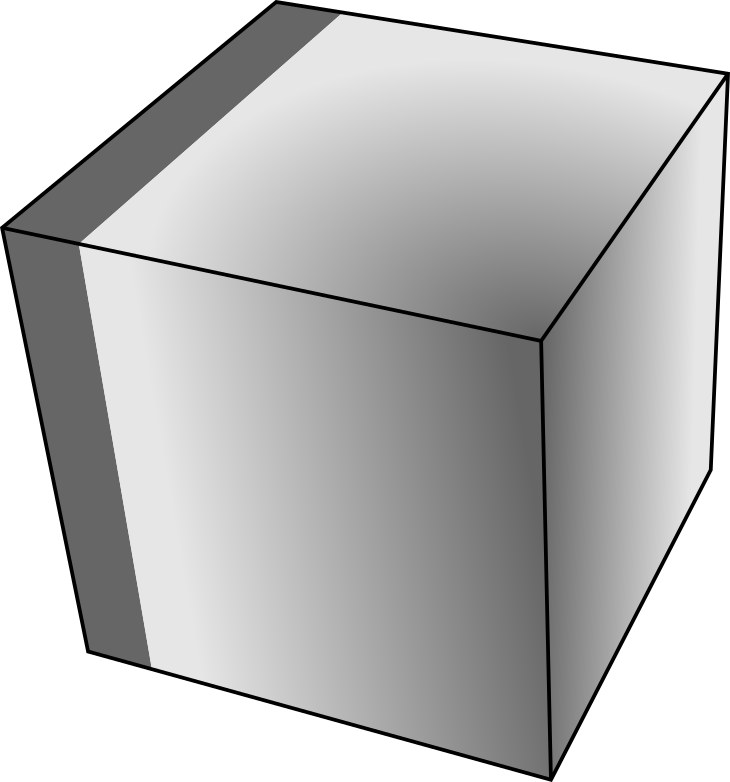
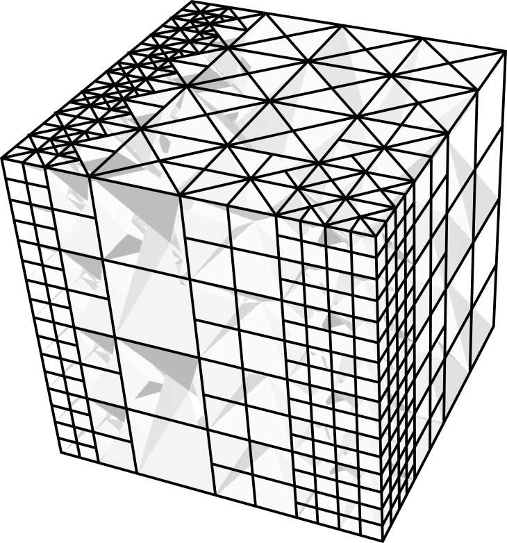
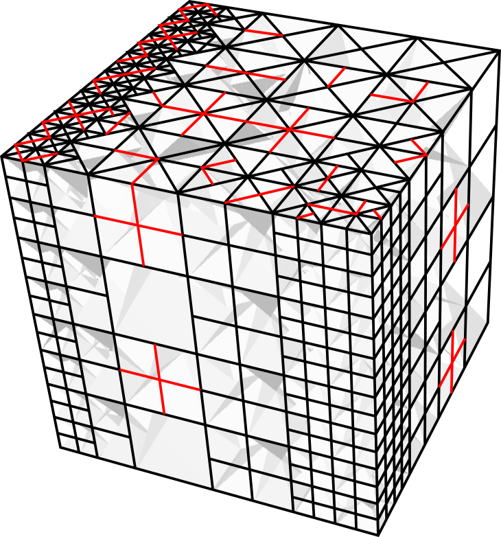
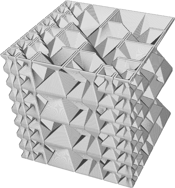
In this paper, we propose a novel type of foam structure that can achieve the aforementioned objective. Specifically, we develop a space-filling surface, called CrossFill, an FDM printable foam structure as infill for a 3D model. Each layer of CrossFill is a space-filling curve that can be continuously extruded along a single overlap-free toolpath. The space-filling surface consists of surface patches which are embedded in prism-shaped cells, which can be adaptively subdivided to match the user-specified density distribution. The adaptive subdivision level results in graded mechanical properties throughout the foam structure. Our method consists of a step to determine a lower bound for the subdivision levels at each location and a dithering step to refine the local average densities, so that we can generate CrossFill that closely matches the required density distribution. A simple and effective algorithm is developed to merge a space-filling curve of CrossFill of a layer into the closed polygonal areas sliced from the input model. Physical printing tests have been conducted to verify the performance of the CrossFill structures.
Our approach provides three technical contributions:
- •
A novel self-supporting space-filling surface which supports spatially graded density;
- •
A scheme for refining the structure to match a prescribed density distribution;
- •
An algorithm for merging the toolpath of an infill structure with the input model’s boundary so as to retain continuity.







2 Related work
For an overview of techniques involved in 3D printing let us refer to the survey articles by Attene et al. 2018 and Livesu et al. 2017. In this section we review the design of microstructures and in particular for extrusion-based 3D printing, as well as the use of space-filling curves and surfaces.
2.1 Structures with graded properties
A variety of graded structures have been proposed in recent years, including lattice structures with varying thickness (e.g. [3, 4, 5, 6, 7]), triply periodic minimal surfaces (e.g. [8, 9]), free-form microstructures [10], microstructures for expressive deformation (e.g. [11, 12, 13]), bone-like microstructures (e.g. [14, 15]) and microstructures optimized by inverse homogenization (e.g. [16, 17]).
Most of these complex structures are fabricated with powder-based 3D printing systems such as selective laser sintering (SLS) or with stereolithography (SLA). Density gradation is typically achieved by varying the thickness of geometric primitives. However, reliably fabricating microstructures with varying thickness is challenging for extrusion-based 3D printing. When printing beads narrower than the nozzle size, it is difficult to predict at which location exactly the bead will end up; furthermore, when the geometry is wider than the nozzle size the toolpath generation needs to switch from a single bead into several in a controlled manner. Furthermore, lattice structures are sliced into small disconnected components for each layer which violates the continuous extrusion constraint (e.g. [3, 12, 18]).
2.2 Structures for extrusion-based printing
3D shapes fabricated by FDM typically comprise uniform infill structures. Recently Martínez et al. 2018 proposed a method to generate infill structures with spatially graded density by printing the cell membranes of 3D Voronoi diagrams. The cells center locations are randomly sampled from a 3D user-specified probability distribution in order to create the spatially graded infill. Overhang constraints are satisfied by carefully constructing a distance measure which forms the basis of defining the cell membranes.
The generated structures are limited by the following factors. The extrusion paths are not continuous; the amount of retractions reduces reliability and increases print time. The density is controlled indirectly through the density of the cell centers. The actual relation between the two remains unclear. At high densities the method is likely to generate overlapping extrusion paths, leading to over-extrusion, which causes defects in the print. These problems are well resolved by our approach.
Wu et al. 2016 proposed using a subdivision grid of slanted cubes called rhombuses for extrusion-based 3D printing and proposed optimizing the subdivision structure for stiffness [21]. The sides of the rhombuses can then be printed using a single bead. However, the T-junctions require retractions, which are problematic especially for flexible materials. Our method makes use of a subdivision grid as well, but generates a continuous toolpath. Moreover, compared to the rigid rhombic structures, the CrossFill structure is more compliant and acts like a foam, which is beneficial for several applications such as an insole.
2.3 Space-filling curves and surfaces
Our method makes use of space-filling surfaces, which are analogous to space-filling curves in 2D (e.g. Hilbert curve [23], Sierpiński curve [24, 25]). Using space-filling curves with varying degrees of subdivision level has been explored for purposes other than 3D printing, such as robotic exploration tasks [26], finite element analysis [27, 28], paths for CNC milling [29]. In the context of 3D printing, Kumar et al. 2009 combined several square based space-filling curves (e.g. Hilbert curve) to generate porous infill structures with spatially graded density and semi-continuous extrusion. However, this method allows for spatially varying density only in the horizontal plane - not in the vertical direction.
While there is much literature on extending such space-filling curves to polylines in 3D, a space-filling curve in 2D can also be extended into a space-filling surface in 3D. Space-filling surfaces are first defined by Ahmed and Bokhari 2007. Although the space-filling surfaces are continuous, any layer-wise cross section is still discontinuous. In this paper we propose a new type of space-filling surfaces, which provides cross sections that are continuous.
3 Overview
CrossFill is a space-filling surface that is constructed using subdivision rules on prism-shaped cells. Each cell contains a patch of the surface, which is sliced into a line segment on each layer to be a segment of the extrusion toolpath. Since the toolpath will be fabricated with a constant width, the size of a cell determines the regional fraction of solid material (hereafter referred to as ‘density’). By adaptively applying the subdivision rules to the prism cells, we create a subdivision structure of cells with a density distribution that closely matches a user-specified input. Continuity of the space-filling surface across adjacent cells with different subdivision levels – both horizontally and vertically – is ensured by the subdivision rules and by post-processing of the surface patches in neighboring cells.
Figure 3 provides an overview of our method using a simple 3D example (bottom) and a 2D schematic illustration (top). From a user-specified 3D density field (Fig. 3(b)), we first increase the subdivision levels everywhere until one further subdivision would result in an average cell density higher than the average requested density in that region (Fig. 3(c)). The resulting subdivision structure forms the lower bound of the final subdivision levels. In order to closely match the input density distribution, we develop a dithering method in which we alternate the subdivision level between the lower bound and one level deeper (Fig. 3(d)). Once the subdivision structure is finalized, we slice it into space-filling curves for the toolpaths on each layer (Fig. 3(e)). In this step, we adjust the surface patches in the cells such that overlapping toolpaths are prevented. Lastly, the space-filling curves are trimmed to the infill area and connected to the shell of the input 3D models to form the final toolpaths preserving continuous extrusion (Fig. 3(f)).
4 CrossFill
CrossFill is an infill structure which consists of a space-filling surface. CrossFill is so named because the toolpath of this structure resembles crosses (see Fig. 9).
4.1 Initialization and data-structure

The space-filling surface of CrossFill is generated using a subdivision scheme that starts from a cube which encompasses the input 3D model with side lengths for integer values of and a constant extrusion width . This cube is divided into four prisms by splitting along the two diagonals of the horizontal faces. Starting from these four prisms, the prisms are adaptively subdivided into smaller ones. In lieu of the commonly used 1:8 subdivision of cubic cells, we make use of 1:2 and 1:4 subdivision of prism-shaped cells. This allows more granularity, which is beneficial for matching the requested density distribution. Details on the types of prism-shaped cells and subdivision rules will be presented in Section 4.2 and 4.3, respectively.
The hierarchy and connectivity of cells are encoded by a combination of a tree and a graph. The subdivision tree connects a cell to its subdivided constituent cells. The root node of the tree corresponds to the starting cube, while other nodes correspond to prism cells. The leaf nodes of the tree constitute the current subdivision structure. The connectivity graph stores the connectivity information among the leaf cells. Two neighboring leaf cells are linked if their surface patches are connected through the space-filling surface; however, two cells which share a face which is not crossed by the space-filling surface are not linked. The links store the relative spatial location of the neighboring cell – up, down left or right along the space-filling surface. See Fig. 4 for an illustration. This connectivity graph facilitates efficient traveling between neighboring cells. The tree and graph are updated each time a new subdivision is applied to a leaf node.
4.2 Types of cell
The construction of CrossFill depends on a subdivision tiling consisting of prism-shaped cells. As shown in Fig. 5, two types of prism are distinguished in our subdivision system:
- H-prism
-
is constructed by vertically cutting a cube in half along a diagonal of the horizontal faces.
- Q-prism
-
is generated by splitting a cube into quarters along both diagonals of the horizontal faces.
The subdivision tiling is generated by subdividing an H-prism into two Q-prisms and subdividing a Q-prism into four H-prisms (see the bottom row of Fig. 5).
Each prism cell encompasses a triangular patch of the space-filling surface. The prism cells are categorized according to which side faces of the prism are crossed by the triangle surface patch (see the horizontal cross sections visualized in Fig. 7(a)):
- A-route
-
the surface is spanned across the faces connected to the two catheti of the right triangle at the base of the prism.
- L-route
-
the surface crosses between the face connected to the hypotenuse and the left cathetus.
- R-route
-
the surface crosses between the face connected to the hypotenuse and the right cathetus.
In order to keep track of the spatial ordering between cells when subdividing and when updating the connectivity graph, we introduce the horizontal direction of traversal (see Fig. 6):
- direction
-
travel from left to right, from left to hypotenuse or from hypotenuse to right.
- direction
-
travel from right to left, from right to hypotenuse or from hypotenuse to left.
In order to fully characterize a cell, we also distinguish between the two fashions in which the 3D surface patch is embedded in the prism (compare the bottom and top in Fig. 6):
- E-embedding
-
when vertically exploring a cell from bottom to top by horizontal cross sections, the embedded surface is said to be expanding if it is moving from the right of the traveling direction to the left.
- C-embedding
-
the embedded surface is contracting otherwise. (Note that the embedding is not defined in terms of whether the triangle surface patch points up or down.)
In total we consider 12 different types of prism cell; see Fig. 6. It can be easily verified that the overhanging angle of embedded surfaces in all types of prism cell is always less than – i.e., the self-supporting constraint is satisfied.
4.3 Subdivision rules
We now define the subdivision rules on the prism cells, which depend on the type of prism (H- or Q-prism), the route type (A-, L- or R-route), the direction of traversal ( or ) and the type of embedding (C- or E-embedding):
| (1) |
where the pattern ‘’ can be filled with any of the subrules for route type and traveling direction as given in Fig. 7(b). The spatial ordering on the right hand side of the rule indicates the spatial ordering of the cells: on top of each other and horizontally next to each other when following the route along its direction. Two examples of filled subdivision rules described by Eq. 1 are illustrated in Fig. 8.
We initialize the CrossFill fractal with four QCA- cells such that the surface patches form a pyramid. Together with the subdivision rules this forms a system closely related to an L-system.
Relation to 2D L-systems
As illustrated in Fig. 9(a) and 9(b), a subdivision tiling of right triangles and an embedded 2D space-filling curve can be obtained when intersecting a uniformly subdivided CrossFill structure with a horizontalplane at an altitude of half the prism’s height. The rules used above with integrated traversal information can help generate a 2D space-filling curve similar to the Sierpiński curve (see the purple curve in Fig. 9(c)). Whereas the Sierpiński curve is generated by connecting the centers of the triangle cells, the CrossFill pattern is generated by connecting the vertices located on the edges which are crossed by the curve. Compared to the 1:4 subdivision of square cells (e.g. for constructing the Hilbert curve), the 1:2 subdivision of triangles allows more granularity. Similarly, our 3D subdivision rules provide more granularity than a cubic 1:8 subdivision. As illustrated in Fig. 10, repeatedly denser space-filling curves can be obtained when reapplying the subdivision rules defined in Fig. 7(b).
4.4 Compatibility and continuity
The surface patches embedded in a subdivision structure with uniform subdivision level form a continuous space-filling surface. With adaptive subdivision levels, neighboring cells can have different sizes. The boundary of the surface patch embedded in a big cell does not always match with the boundary of surface patches in neighboring linked smaller cells (e.g. prisms 10 and 27 in Fig. 4).
To solve this problem in general is difficult; however, it is solvable when neighboring linked cells have only one level difference in the subdivision tree, because there is only a limited set of configurations. The continuity can be enforced on such a structure with heterogeneous subdivision level in three steps.
Step 1: Horizontal continuity enforcement
When horizontally neighboring cells have a different subdivision level their embedded surface patches may not match at the sides where the cells meet. For example the edge in Fig. 11 doesn’t align with and . In such a case the edge of the lower subdivision level cell is transformed such that it matches the higher subdivision level cells and its surface is converted into a ruled surface : on each layer we connect the one edge () of the surface patch with either of the two edges ( or ) of the smaller surface patches using a horizontally straight line segment. See Fig. 11 and Fig. 12(a).
Step 2: Vertical side continuity enforcement
When vertically neighboring cells have a different subdivision level the edges of their surfaces may not end in the same location at the interface where the cells meet. For example the vertex doesn’t coincide with in Fig. 11. In such a case the edge(s) of the lower subdivision level cell are transformed: part of the edge is flipped horizontally in the plane along the cell side where the edge resides. This adjustment is also performed if the discontinuity was introduced because of the horizontal continuity enforcement, as is illustrated by surface patch in the middle of Fig. 11.
Step 3: Vertical mid continuity enforcement
When vertically neighboring cells have different subdivision level and have ruled surfaces the horizontal edges may not align on the horizontal side where the cells meet. For example vertex doesn’t lie on the edge in Fig. 11. In such a case the vertices of the higher subdivision level cells are adjusted to lie on the intersection between edge and the side where the two higher subdivision cells meet horizontally. Similar to vertical side continuity enforcement, we flip part of the edge to which the adjusted vertex belongs and introduce ruled surfaces.
The space-filling surface in linked cells with subdivision level differences can be effectively enforced to be continuous by this approach. Examples of CrossFill structures with continuity enforcement are shown in Fig. 12. For more extensive examples we refer to the video in the supplementary material. Note that in the implementation we do not actually construct the surface; instead, we compute the vertex locations of the edge segments of the surface patches, slice those at the height of a printing layer and connect the resulting locations using straight line segments.


Self-supporting
It should be noted that the curved surfaces introduced by enforcing the continuity of neighboring linked prism cells will not violate the self-supporting property of the space-filling surface. With the help of the carefully designed continuity enforcement algorithm, we generate surfaces that have overhang in most places. There is only one exceptional case for the side enforcement in an H-prism, where the overhang can be increased to . However, geometry overhanging with an angle of is not a problem for most FDM 3D printers, so the self-supporting constraint is not violated.
Density
Sudden jumps in density are hard to be realized on our infill structure. For example, a density distribution which is in the bottom half and in the top half is not easily realized while satisfying the overhang constraint. Our space-filling surface requires some distance to change from the low to the very high density along the vertical direction. Also, the surface patch with enforced continuity would be considerably different from the original triangular surface patches, which might have a large influence on the physical properties associated with a given density. The situation is controlled by imposing the constraint that cells linked to each other only allow to differ by a single subdivision level at most.
The distance required to change from a low density to a high density depends heavily on the size of the cell associated with the lower density. For a simple square subdivision grid the distance between the side of a cell with subdivision level and height to a cell with subdivision level is minimally , which converges to for . For our prism based subdivision approach the distance converges to vertically and horizontally. However, depending on the positioning of the most dense cell w.r.t. the grid of the least dense cell, the required distance can increase to vertically and horizontally. The horizontal distance is measured along the space filling surface in terms of the average length of segments in the 2D L-system. This means that two cells which are spatially next to each other can have a large difference in density so long as the space filling surface takes a large detour between the two.
5 Adaptive subdivision
This section presents our approach for generating a subdivision structure with subdivision levels which closely matches the requested density distribution. Our approach consists of two steps: the first decides a lower bound subdivision level at each location and the second fine-tunes the local density distribution by dithering between the lower bound and a higher bound. Before presenting this approach, we introduce the methods for evaluating the target and the current density in a cell.
5.1 Target cell density
Common ways of specifying a density distribution are as a scalar field defined on a tetrahedral mesh or a voxel model or as a procedural function. In order to make our program compatible with several commercial software packages, we construct a voxel model from a sequence of gray-scale image files. The relationship between the gray-scale value and the physical density is specified by the user. The target density of a cell is computed as the average density of voxels covered by :
| (2) |
where the function computes the volume of the common region of a voxel and a cell . We define the target mass as the requested amount of volume to be filled with solid material in a cell:
| (3) |
Because the size of starting cube of CrossFill is a power of times the extrusion width , the fractal can start with a volume which is considerably larger than the input model and its density distribution. For a cell lying completely outside the voxel set, we use the density of its nearest voxel as its density .
5.2 Current cell density
For a cell located at level in the subdivision tree, we calculate the current amount of material in the surface patch according to the size of and the type of route (L, R or A). By considering the configurations of embedded triangles in a prism cell (Fig. 6), we calculate the current density estimate of and the corresponding current mass as follows:
| (4) |
where is the constant width of material extrusion, is the length of the cathetus at the top of the prism and is the side length of the starting cube. Note that is the horizontal width which differs from the thickness in the direction normal to the surface. Note also that the density, i.e., the fraction of solid material, is independent of the height of the prism, the embedding of the surface patch and the direction; it is determined by the average of horizontal segment length and the extrusion width , which are unaffected by these factors. In this analysis, for the sake of simplicity, we neglect the effect that linked cells influence the density of a given cell due to the continuity enforcement. We provide a method for compensating for the errors induced by continuity enforcement in Section 7.1.1.
From Eq. 4 and the subdivision rules in Fig. 7 we can derive the increment in mass when performing a subdivision, which is used to supervise the generation of an adaptive subdivision structure. The new mass the children cells would have after a subdivision is as follows:
| (5) |
The ratio of A-, L- and R-route cells in a CrossFill structure with uniform subdivision level quickly converges to after a depth of only 5 subdivisions. If the current density of A-route cells is then the other of all cells is still at a lower density, so the maximum attainable density in the whole structure is .
From the above we can derive that the average density increment factor is . This provides more granularity than other fractal structures, e.g. the Hilbert curve, which has a density increment factor of for each subdivision. One step of the Hilbert curve quadruples the amount of cells, while it only doubles the distance between connected cells, so the total length of the curve is doubled, which means that the curve with a constant line width comes to cover double the area.
5.3 Lower bound subdivision levels
Given the specified density distribution, we adaptively refine the subdivision structure such that the current density of each cell approaches, but does not exceed, the average target density (i.e., Eq. 2). This is achieved by a top-down pass on the subdivision tree. In order to accomplish that we subdivide a cell if it satisfies the following condition: . To restrict the subdivision level difference between linked cells to be at most one, before subdividing a candidate cell that satisfies the condition, we subdivide its linked cells with a shallower subdivision level first.
The pseudo-code of our algorithm is presented in Algorithm 1. By calling the function LowerBoundSubd() on the root of the tree, the subdivision level is decided in each location. This constitutes the lower bound subdivision levels. The following subsection presents a dithering approach to further reduce the approximation error.
5.4 Dithering
Because the input is a continuous density distribution while the output only admits a limited set of subdivision levels, choosing a subdivision level of a CrossFill cell always induces a discretization error a.k.a. quantization error. The idea is to diffuse this quantization error to linked cells in the neighborhood so as to influence the chosen subdivision level there. This causes the subdivision levels to oscillate between the subdivision levels closest to the target density (see Fig. 13). This is akin to the widely employed dithering technique in multimedia processing.
We define the quantization error as the difference between target mass and current mass. Diffusing this error to dither the subdivision level leads to a CrossFill structure with densities better matching the target distribution regionally. See Fig. 14 for an example on a simple square subdivision tiling. The lower bound subdivision structure exhibits strong banding artifacts; these artifacts are eliminated by dithering.


Dithering order
When processing cells for dithering we consider the leaf nodes in a sequence analogous to the Morton order [32]: We traverse the tree in depth-first order and at each non-leaf cell we recurse the children in the following order: first the bottom left, then the bottom right and, if it is a Q-prism, then the top left and the top right. Here ‘right’ refers to linked cells along the direction of the horizontal traversal of the surface patches, which is clockwise around the space-filling polygon of each layer. Quantization error of the current cell is then redistributed to those cells in the neighborhood of which have not yet been processed in dithering.
Neighborhood
Dithering along a manifold with a lower dimension makes the implementation simpler while retaining the advantages of dithering. Velho and Gomes 1991 [33] have shown that propagating quantization error along the directions of a space-filling curve (as 1D manifold) for 2D images can yield a halftoning technique with appealing properties. Similarly, rather than considering all geometrically neighboring cells of a prism cell , we only consider the cells which are neighboring in the connectivity graph. As such we only disperse quantization error along the 2D manifold of the space-filling surface within 3D space. In order to visualize the dithering process effectively, we ‘unfold’ the space-filling surface and consider the resulting 2D topology (see Fig. 4(a) and the supplementary video).
Weights
The amount of the quantization error distributed to each (yet unprocessed) cell in the neighborhood depends on its relative position with respect to the current cell being checked. Connected cells to the left and bottom have always already been processed because of the Morton order. For a subdivision structure with uniform subdivision, the configuration is therefore as shown in Fig. 15(a). The diagonal cells are obtained by accessing the links of directly linked neighbors. There are various error diffusion schemes with different weights and different configurations (ref. [34, 35, 36]). A comprehensive study about their performance is beyond the scope of this paper. We employ a simple error diffusion scheme with the following weights: , and . Because not all positions relative to the checking cell are always occupied by (unprocessed) cells, the weights are normalized to compute the quantization error to be diffused to unprocessed linked neighbors:
Because linked cells can have a size different from , the weights need to be adjusted to account for the change of configuration. A linked cell can occupy more space than or only a portion of the space occupied by . In the former case multiple weights are added together, while in the latter case the weight is split equally. The diagonal positions always retain the same weight. An illustration of such a configuration can be found in Fig. 15(b).
Algorithm
The dithering algorithm decides on the final subdivision level by choosing between the lower bound subdivision level and a higher bound of one subdivision level deeper by comparing the quantization error of those two subdivision levels. The quantization error of a prism cell before subdivision () and after subdivision () are calculated by
| (6) |
where is the quantization error diffused to from already processed cells. is subdivided if the absolute value of is smaller than the absolute value of . An exception to this rule is if has linked neighbors with a lower subdivision level in order to comply with the constraint that linked cell can only differ by a single subdivision level. After the subdivision decision the corresponding quantization error is diffused to the unprocessed linked neighbors according to the weighing scheme described above. Pseudo-code of this dithering approach is given in Algorithm 2. The diffused error is initialized as zero on each cell before calling Dither on the root of the subdivision tree. Figure 14(c) shows the result on a 2D example.
6 Toolpath generation
We now have a method for creating an infill structure with spatially graded density according to a user-specified density distribution. The infill structure is defined in a cubic region and can be fabricated by continuous material extrusion. In this section, we will first explain how to effectively slice the structure into a continuous 2D polygonal curve for each layer. After that, we will fit the 2D polygonal curve of a layer into the region of an input 3D model.
6.1 Slicing
The first step toward generating the toolpath of a layer for 3D printing is to generate the space-filling curve which lies on the intersection between the surface of CrossFill and the horizontal plane at the height of the printing layer. As mentioned above, the space-filling surface only exists conceptually in our implementation. We directly generate the space-filling curves from the type of prism cells and their linkage in the connectivity graph. Given a height , we first find the sequence of cells covering this height in the subdivision structure. The cell which is closest to the last point on the toolpath of the previous layer, is chosen as the first cell for exploring the horizontally linked cells. The whole sequence of cells can be traced out by following the links in the connectivity graph which are pointing to the right, i.e., by following the cells along the horizontal traversal direction (see Fig. 6). When appending a cell to the sequence we take take the right linked cell which intersects with the height. After employing the continuity enforcement rules from Section 4.4 we are left with the edges of the surface patches, which are sliced at to serve as the vertices of the space-filling curve of that layer.
6.2 Overlap prevention
These space-filling curves can have overlap near the boundary of a prism when a surface patch segment is too close to the neighboring prism (see Fig. 16(a) for an example). This occurs when the distance between the two segments is less than the horizontal width of extrusion toolpaths. In order to prevent path overlap, we clamp the endpoints of sliced line segments to a position that is away from the neighboring prism (see Fig. 16(b)).
However, only applying the clamping step cannot completely avoid overlap in situations where the toolpath makes a sharp turn. When the turning angle between the segment and the side of the cell is sharper than , we introduce an additional vertex at a position with distance away from the vertex on the side of the cell – called detouring. See Fig. 16(c). It should be noted that in a uniformly subdivided CrossFill structure, the turning angle on a space-filling curve generated by slicing is either or (see Fig. 9(b) for an example), which means that detouring is not needed in such a context.
Detouring does not violate the overhang constraint. The introduced vertex is supported either by a detoured vertex below or a segment with a turning angle just above . Moreover, detouring does not reduce any area covered by the extrusion path, so a detoured layer still supports the layer above. The increased density caused by detouring can be compensated for using a method introduced in Section 7.1.1.
6.3 Conversion into infill structure
Now that we have a non-overlapping space-filling curve as toolpath for fabricating the CrossFill structure of each layer, We limit it to the interior area of an input 3D model while retaining the continuity of the toolpaths. Specifically, we first intersect the space-filling curve with the infill area shrunk by (see Fig. 17(c)). This operation makes the trimmed space-filling curve connected to itself via the perimeters of that layer.

Performing an intersection between the space-filling curve and the infill area could result in a single polygon. However, there are cases in which additional polygons are generated:
- 1.
the infill area splits the space-filling curve into multiple parts (in the bottom right of Fig. 17(b));
- 2.
the infill area contains a polygon which doesn’t touch the space-filling curve (in the top left of Fig. 17(b)).
We tackle both these problems by connecting all polygons to the innermost perimeter of the shell of the print and to each other afterwards. The problem to be solved here for generating continuous toolpaths is different from [37], in which spiraling toolpaths are generated to completely fill a given region. By contrast, we are tackling the problem of connecting multiple polygons into a single polygonal curve.
Two polygons are connected into a single polygon by building a bridge between them as follows. First, two points and with on a polygon are considered. We consider the point on the other polygons closest to and find a point on the other polygon such that is parallel to . We search for such pairs of points until we find a bridge for which the length is at most . New line segments and are then added and the line segments and are removed. Examples for building bridges can be found in Fig. 17(d). Repeatedly building bridges between polygons can connect all into a single polygon. In order to minimize the number of sub-optimal bridges, we start by connecting the smallest polygons to suitable neighbors and work our way outward.
Our method has several advantages. When there are many possible candidate locations for building a bridge, we can select the ‘optimal’ position according to various criteria. For example, we can promote bridges at regions with low curvature in order to minimize the influence on the extruded amount of material. Another option is to build bridges that are closer to interior regions so as to minimize the visual surface impact.
Connecting polygons which have distance more than introduces new line segments hanging in the air. Strictly this conflicts with the overhang constraint; however, this often is not a problem for FDM printing. Such distances are rarely long, and these lines of bridges do not have to support any material above. In practice, the extruded beads of FDM can stay in mid-air because of the high viscosity of the melted plastic.
7 Results
7.1 Experiments
Experiments were performed on an Intel Core i7-7500U CPU @ using a single core and memory. We have printed test structures on several Ultimaker 3 machines, loaded with white Ultimaker TPU 95A in AA Print Cores. The basic print path settings were taken from the default Cura 4.0 profile of layer thickness for this setup. qMost notably the setting for Infill Line Width was and the Speed was . In order to enable the connect polygons functionality in some of our tests, we set the Extra Skin Wall Count to zero and instead set the Extra Infill Wall Count to one, so that we can enable the setting Connect Infill Polygons. The Infill Line Distance setting was set to meaning that the smallest possible prism has sides of length , which corresponds to a density of in order to save computation time.
For various tests we have used a test cube with side lengths of , which is , so that the starting cube of the subdivision tree matches the 3D model. In order to isolate the infill structure, the settings Top/Bottom Thickness and the Wall Thickness have been set to .
For some of the models, the requested infill densities are too low to support the dense top skin. In order to overcome this problem, we enforced a minimal subdivision level for prism cells which overlap with top skin after the dithering stage, by iteratively calling Subdivide from Algorithm 1. By modifying the subdivision structure in this way, we guarantee a required percentage of infill for supporting top skin regions.
7.1.1 Simplified density measure compensation
The method we propose uses a simplified density estimate based on cell size and route type. Because this doesn’t take into account effects from continuity enforcement (Section 4.4) or from clamping and detouring (Section 6.2) the output density is different from the simplified density estimates. Once we evaluate the discrepancy, we can compensate for it.
We have generated test cubes with a homogeneous simplified density (Eq. 4) within the range of to and analyzed the total extruded volume compared to the total volume of the cube. These results are shown in blue in Fig. 18. We fit a Matlab smoothing spline to the data with a smoothing parameter of . The resulting curve is then used to compensate for the disparity between the simplified density estimates and the actual densities by mapping the density requirements to the corresponding simplified density estimates prior to applying our algorithms.
7.1.2 Accuracy
The accuracy of a functionally graded material is inherently related to a viewing resolution. When viewing any print at a resolution close to the printer resolution, the density is either or regardless of the user specified density at each location, which means the accuracy at that resolution is low. In order to evaluate the accuracy of our functionally graded material, we evaluate the average local error at a range of resolutions. For each resolution we divide the specification and the generated infill structure into smaller cubes and compute the local error as the absolute difference between the average specification density throughout that cube and the average realized density throughout that cube. The accuracy is then given by the average local error across all subcubes for that resolution (see Fig. 19). Note that at kernel sizes of powers of two the subcubes align with the prism-shaped cells, which lowers the error measure.


We define several density specifications for our test cube on which we evaluate the accuracy. a) Homogeneous at . b) Homogeneous at . c) Gradient: a smooth linear gradient from in one bottom corner to in the diametrically opposite corner. d) Contrast plane: half of the cube is infill density and the other half is . The plane which separates these two halves makes an angle of with the X axis in the horizontal plane and has an overhang angle of . e) Sphere shell: a sphere with a radius of half the cube side length and a shell thickness of 1/7 the size of the side lengths of the cube. The density of the shell is and the density inside and outside is . All these are specifications consisting of images of . The accuracy results are shown in Fig. 20.
7.1.3 Computation time
In order to evaluate the running time of our algorithms, we consider four of the application models discussed in Section 7.3. We consider the test models and corresponding settings displayed in Table 1. The computation times are shown in Table 2.
| white | black | top | spec size () | phys. size () | |
|---|---|---|---|---|---|
| Sole | |||||
| Bunny | |||||
| Phantom | |||||
| Saddle |
| Sole | Bunny | Phantom | Saddle | |
| Lower bound | 6.2 | 11.2 | 4.3 | 150.9 |
| Dithering | 0.5 | 2.3 | 0.4 | 10.5 |
| Extract polygon | 0.4 | 15.7 | 3.4 | 12.8 |
| Limit polygon | 0.3 | 11.3 | 3.8 | 12.0 |
| Reconnecting | 4.6 | 98.9 | 65.4 | 135 |
| Total gcode | 14 | 182 | 105 | 346 |
7.1.4 Elastic behavior
Because the generated structures are similar to foams, which are often used in a compressive context, it would be interesting to find out their compressive behavior. Because the non-linear material properties at high strain values when compressing a foam are difficult to capture when using a finite elements method, we have performed actual physical tests instead.
We have printed samples with homogeneous subdivision level, and we have printed samples using dithering to approximate several homogeneous density specifications with simplified densities between and . Compressions were performed in both the vertical and the horizontal direction. Because our structures are rotationally symmetric around the Z axis we only need to test 2 of the 3 dimensions. In total 78 prints were made in 42 test configurations (some configurations were tested multiple times): 2 testing directions, 4 homogeneous subdivision levels (, , , ) and 17 heterogeneous subdivision levels in the same range.


We have performed compression tests on the Instron 3366, fitted with compression plates. See Fig. 21(a). Compressions were performed at a speed of up to a maximum force of after which the sample was decompressed.
The stress-strain results are plotted in Fig. 22. One interesting observation from the data is that the stress-strain graphs are roughly horizontal for a long range of strain values. This is caused by the structure collapsing and folding in on itself. Such plateaus are typical of foams [38, 39], and they are important design variables for common applications of foams [40]. Figure 21(b) shows how such collapse can be localized to only a particular Z range in the case of vertical compression.
The constant stress along that range is a fundamental characteristic of such a plateau. We estimate it by taking the average stress along the part of the stress-strain graph which has a local tangent modulus below . The resulting values have been plotted alongside the Young’s modulus values in Fig. 23(b).


7.2 Discussion
Accuracy
At a kernel size of () the average absolute local error is low for smooth input density distributions. Because of the constraint that neighboring linked cells can only differ by a single subdivision level the two distributions with sharp contrast edges or high frequency detail score considerably worse. See Fig. 20, ‘contrast plane’ and ‘sphere shell’. The relative error decreases as the resolution increases. Therefore, depending on the application the user might decide that at a specific resolution the accuracy is good enough.
Computation time
Our algorithms take up over of the total gcode generation time; there is room for improvement. It should be noted that we not optimized the code for loading the density specification data into the subdivision tree or the code for connecting polygons, which currently consume the majority of the processing times. Polygon extraction and polygon limiting times depend highly on the number of layers, which is relatively small for the shoe sole example.
Elastic behavior
It should be noted that the first local maximum in the stress-strain graphs of Fig. 22 are not the yield points. Most of the deformation applied to the structure is elastic deformation. We observed the material to creep back to its original shape at ever decreasing rates. After hours a strain of merely remained after an initial strain above , meaning that the plastic deformation is negligible at stresses with magnitudes as high as in our tests ().
For larger densities the strain at which the structure is fully collapsed is lower. When we compress a sample with density by then the stress-strain graph should exhibit a local tangent equal to the base properties of the material used. In our test results we see that the tangent tends toward the Young’s modulus of TPU: [41]. This agrees with literature on the densification of foams [38].
In most aspects the structures are more compliant in the vertical direction than in the horizontal. The plateau heights in Fig. 22(a) are lower than the corresponding ones in 22(b) and the strain regions of the plateaus are wider as well. Of course some aspect of this anisotropy is caused by the layerwise buildup of FDM, but a larger part of the difference is most likely caused by the geometric structure. The structure can collapse in the Z direction easily because of the alternating E- and C-embeddings.
The vertical Young’s modulus is lower than the horizontal Young’s modulus for most densities. For densities around and , that relationship is reversed, though. That can be explained by the fact that around those densities the subdivision structure contains mostly Q-prism cells which are filled with CrossFill surface patches with a more vertical slope than those for H-prisms. More vertical elements increase the stiffness in the vertical direction.
The prisms only subdivide vertically every two iterations: only the Q-prisms do. The H-prisms of are subdivided horizontally compared to , while the prisms of and are also subdivided vertically compared to and respectively. This irregularity can explain the nonmonotonicity we see in the Young’s modulus with respect to infill densities in Fig. 23(b): horizontal subdivision decreases the slope of the surface patches in the structure, which decreases the thickness of these patches, which in turn decreases the overall stiffness.
Because the deeper subdivision level cells determine the ruled surface in horizontal continuity enforcement, surface patches of a dithered subdivision structure are predominantly determined by the higher density cells. We therefore expect to see large changes after and after . We can see large jumps in the vertical Young’s modulus at those places in Fig. 23(b). Also the plateau heights for horizontal compressions show large jumps.
When comparing the dithered results in Fig. 23 to the ones without dithering we can conclude that dithering indeed provides more granular control of the overall material properties of the manufactured part. However, because of the nonmonotonicity in these results it is not trivial to define a process for the designer to choose which infill density is needed at a location in a design.
7.3 Applications
The structures generated by our method support variable compliance, which can control the deformation of an object under certain loads. We have designed a density specification for the Stanford bunny model using Autodesk Monolith [42], as shown in Fig. 24d.
Because the CrossFill structures behave much like foams, it could be attractive for "cushioning, packaging and energy absorption" [38]. Foams with variable stiffness could be used for a personalized bike saddle (see Fig. 24a) or for personalized shoe soles (see Fig. 24c).
A boundary mesh of a teddy bear along with a density distribution show how different densities lead to different bending behavior (see Fig. 24b). The difference in density distribution in the two arms causes the arms to deform in a different way under the same load.
Because our method is principally density-based, it could also be useful in situations where the relevant material properties are volumetric; CrossFill could prove useful for imaging phantoms - objects which can be used in the medical field to evaluate magnetic resonance imaging (MRI) scan procedures. We have printed an example of what could serve as a phantom in Fig. 24e.
8 Conclusion and future work
In this paper, we have introduced a new infill structure, CrossFill, which can provide spatially graded density to match a user-specified density distribution. CrossFill is carefully designed so that it is self-supporting and can be fabricated from a single, continuous and overlap-free toolpath on each layer. Algorithms for generating the lower bound subdivision levels and dithering the subdivision levels have been developed to accurately match the prescribed density distribution. To use CrossFill as infill structures of a given 3D model, we have presented an algorithm to connect the toolpaths of CrossFill and the toolpaths for the given model’s shell into a single continuous extrusion path. The performance of CrossFill has been verified on a variety of experimental tests and applications.
The study of experimental tests shows that CrossFill acts very much like a foam although future work needs to be conducted to further explore the mapping between density and other material properties. Another line of research is to further enhance the dithering technique, e.g. changing the weighing scheme of error diffusion.
References
References
- Attene et al. [2018] M. Attene, M. Livesu, S. Lefebvre, T. Funkhouser, S. Rusinkiewicz, S. Ellero, J. Martínez, A. H. Bermano, Design, Representations, and Processing for Additive Manufacturing, Synthesis Lectures on Visual Computing: Computer Graphics, Animation, Computational Photography, and Imaging 10 (2) (2018) 1–146, ISSN 2469-4215, doi:10.2200/S00847ED1V01Y201804VCP031.
- Livesu et al. [2017] M. Livesu, S. Ellero, J. Martínez, S. Lefebvre, M. Attene, From 3D models to 3D prints: an overview of the processing pipeline, vol. 36, Wiley, doi:10.1111/cgf.13147, 2017.
- Martínez et al. [2016] J. Martínez, J. Dumas, S. Lefebvre, Procedural voronoi foams for additive manufacturing, ACM Transactions on Graphics 35 (4) (2016) 1–12, ISSN 07300301, doi:10.1145/2897824.2925922.
- Aremu et al. [2017] A. O. Aremu, J. P. Brennan-Craddock, A. Panesar, I. A. Ashcroft, R. J. Hague, R. D. Wildman, C. Tuck, A voxel-based method of constructing and skinning conformal and functionally graded lattice structures suitable for additive manufacturing, Additive Manufacturing 13 (2017) 1–13, ISSN 22148604, doi:10.1016/j.addma.2016.10.006.
- Bates et al. [2018] S. R. Bates, I. R. Farrow, R. S. Trask, Compressive behaviour of 3D printed thermoplastic polyurethane honeycombs with graded densities, Materials & Design 162 (2018) 130–142, ISSN 02641275, doi:10.1016/j.matdes.2018.11.019.
- Choy et al. [2017] S. Y. Choy, C. N. Sun, K. F. Leong, J. Wei, Compressive properties of functionally graded lattice structures manufactured by selective laser melting, Materials and Design 131 (May) (2017) 112–120, ISSN 18734197, doi:10.1016/j.matdes.2017.06.006.
- Limmahakhun et al. [2017] S. Limmahakhun, A. Oloyede, K. Sitthiseripratip, Y. Xiao, C. Yan, Stiffness and strength tailoring of cobalt chromium graded cellular structures for stress-shielding reduction, Materials and Design 114 (2017) 633–641, ISSN 18734197, doi:10.1016/j.matdes.2016.11.090.
- Li et al. [2018] D. Li, W. Liao, N. Dai, G. Dong, Y. Tang, Y. M. Xie, Optimal design and modeling of gyroid-based functionally graded cellular structures for additive manufacturing, CAD Computer Aided Design 104 (2018) 87–99, ISSN 00104485, doi:10.1016/j.cad.2018.06.003.
- Abueidda et al. [2017] D. W. Abueidda, M. Bakir, R. K. A. Al-Rub, J. S. Bergström, N. A. Sobh, I. Jasiuk, Mechanical properties of 3D printed polymeric cellular materials with triply periodic minimal surface architectures, Materials & Design 122 (2017) 255 – 267, ISSN 0264-1275, doi:10.1016/j.matdes.2017.03.018.
- Massarwi et al. [2018] F. Massarwi, J. Machchhar, P. Antolin, G. Elber, Hierarchical, random and bifurcation tiling with heterogeneity in micro-structures construction via functional composition, Computer-Aided Design 102 (2018) 148–159, doi:10.1016/j.cad.2018.04.017.
- Schumacher et al. [2015] C. Schumacher, B. Bickel, J. Rys, S. Marschner, C. Daraio, M. Gross, Microstructures to control elasticity in 3D printing, ACM Transactions on Graphics 34 (4) (2015) 136:1–136:13, ISSN 07300301, doi:10.1145/2766926.
- Panetta et al. [2015] J. Panetta, Q. Zhou, L. Malomo, N. Pietroni, P. Cignoni, D. Zorin, Elastic textures for additive fabrication, ACM Transactions on Graphics 34 (4) (2015) 135:1–135:12, ISSN 07300301, doi:10.1145/2766937.
- Coulais et al. [2016] C. Coulais, E. Teomy, K. de Reus, Y. Shokef, M. van Hecke, Combinatorial design of textured mechanical metamaterials, Nature 535 (7613) (2016) 529.
- Liu and Shapiro [2015] X. Liu, V. Shapiro, Random heterogeneous materials via texture synthesis, Computational Materials Science 99 (2015) 177 – 189, ISSN 0927-0256, doi:https://doi.org/10.1016/j.commatsci.2014.12.017.
- Wu et al. [2018] J. Wu, N. Aage, R. Westermann, O. Sigmund, Infill Optimization for Additive Manufacturing – Approaching Bone-like Porous Structures, IEEE Transactions on Visualization and Computer Graphics 24 (2) (2018) 1127–1140, ISSN 1077-2626, doi:10.1109/TVCG.2017.2655523.
- Andreassen et al. [2014] E. Andreassen, B. S. Lazarov, O. Sigmund, Design of manufacturable 3D extremal elastic microstructure, Mechanics of Materials 69 (1) (2014) 1 – 10, ISSN 0167-6636, doi:10.1016/j.mechmat.2013.09.018.
- Garner et al. [2019] E. Garner, H. M. Kolken, C. C. Wang, A. A. Zadpoor, J. Wu, Compatibility in microstructural optimization for additive manufacturing, Additive Manufacturing 26 (2019) 65 – 75, ISSN 2214-8604, doi:10.1016/j.addma.2018.12.007.
- Sigmund [1995] O. Sigmund, Tailoring materials with prescribed elastic properties, Mechanics of Materials 20 (4) (1995) 351–368, ISSN 01676636, doi:10.1016/0167-6636(94)00069-7.
- Martínez et al. [2018] J. Martínez, S. Hornus, H. Song, S. Lefebvre, Polyhedral Voronoi diagrams for additive manufacturing, ACM Transactions on Graphics 37 (4) (2018) 15, doi:10.1145/3197517.3201343.
- Wu et al. [2016] J. Wu, C. C. Wang, X. Zhang, R. Westermann, Self-supporting rhombic infill structures for additive manufacturing, Computer-aided Design 80 (2016) 32–42, ISSN 00104485, doi:10.1016/j.cad.2016.07.006.
- Wu [2018] J. Wu, Continuous optimization of adaptive quadtree structures, CAD Computer Aided Design 102 (2018) 72–82, ISSN 00104485, doi:10.1016/j.cad.2018.04.008.
- Martínez et al. [2017] J. Martínez, H. Song, J. Dumas, S. Lefebvre, Orthotropic k-nearest foams for additive manufacturing, ACM Transactions on Graphics 36 (4) (2017) 1–12, ISSN 07300301, doi:10.1145/3072959.3073638.
- Hilbert [1891] D. Hilbert, Ueber die stetige Abbildung einer Line auf ein Flächenstück, Mathematische Annalen 38 (3) (1891) 459–460.
- Sierpiński [1912] W. F. Sierpiński, Sur une nouvelle courbe continue qui remplit toute une aire plane, Bulletin de l’Académie des Sciences de Cracovie - Série A (1912) pp. 463–478.
- Polya [1913] G. Polya, Uber eine Peanosche kurve, Bull. Acad. Sci. Cracovie (Sci. math. et nat. Série A) (1913) 305–313.
- Nair et al. [2017] S. H. Nair, A. Sinha, L. Vachhani, Hilbert’s Space-filling Curve for Regions with Holes, arXiv preprint arXiv:1709.02938 URL http://arxiv.org/abs/1709.02938.
- Gonzaga et al. [2015] S. Gonzaga, O. U. Federal, M. Kischinhevsky, U. Federal, E. N. Methods, M. Kischinhevsky, Sierpínski-like Space-filling Curve for Total Ordering of Adaptive Triangular Discretized Domains (February 2015).
- Bader et al. [2008] M. Bader, S. Schraufstetter, C. Vigh, J. Behrens, Memory efficient adaptive mesh generation and implementation of multigrid algorithms using Sierpinski curves, International Journal of Computational Science and Engineering 4 (1) (2008) 12, ISSN 1742-7185, 1742-7193, doi:10.1504/IJCSE.2008.021108.
- Griffiths [1994] J. G. Griffiths, Toolpath based on Hilbert’s curve, Computer-Aided Design 26 (11) (1994) 839–844, ISSN 00104485, doi:10.1016/0010-4485(94)90098-1.
- Kumar et al. [2009] G. S. Kumar, P. Pandithevan, A. R. Ambatti, Fractal raster tool paths for layered manufacturing of porous objects, Virtual and Physical Prototyping 4 (2) (2009) 91–104, ISSN 17452759, doi:10.1080/17452750802688215.
- Ahmed and Bokhari [2007] M. Ahmed, S. Bokhari, Mapping with space filling surfaces, IEEE Transactions on Parallel and Distributed Systems 18 (9) (2007) 1258–1269, ISSN 10459219, doi:10.1109/TPDS.2007.1049.
- Morton [1966] G. M. Morton, A computer oriented geodetic data base and a new technique in file sequencing, Tech. Rep., IBM, 1966.
- Velho and Gomes [1991] L. Velho, J. d. M. Gomes, Digital halftoning with space filling curves, ACM SIGGRAPH Computer Graphics 25 (4) (1991) 81–90, ISSN 00978930, doi:10.1145/127719.122727.
- Floyd [1976] R. W. Floyd, An adaptive algorithm for spatial gray-scale, in: Proc. Soc. Inf. Disp., vol. 17, 75–77, 1976.
- Jarvis et al. [1976] J. F. Jarvis, C. N. Judice, W. H. Ninke, A survey of techniques for the display of continuous tone pictures on bilevel displays, Computer Graphics and Image Processing 5 (1) (1976) 13–40, ISSN 0146664X, doi:10.1016/S0146-664X(76)80003-2.
- Stucki [1981] P. Stucki, MECCA - A Multiple-Error Correcting Computation Algorithm for Bilevel Image Hardcopy Reproduction, Tech. Rep., IBM Research Lab, Zurich, 1981.
- Zhao et al. [2016] H. Zhao, B. Chen, F. Gu, Q.-X. Huang, J. Garcia, Y. Chen, C. Tu, B. Benes, H. Zhang, D. Cohen-Or, Connected fermat spirals for layered fabrication, ACM Transactions on Graphics 35 (4) (2016) 1–10, ISSN 07300301, doi:10.1145/2897824.2925958.
- Ashby [2006] M. F. Ashby, The properties of foams and lattices, Philosophical Transactions of the Royal Society A: Mathematical, Physical and Engineering Sciences 364 (1838) (2006) 15–30, ISSN 1364503X, doi:10.1098/rsta.2005.1678.
- Avalle et al. [2001] M. Avalle, G. Belingardi, R. Montanini, Characterization of polymeric structural foams under compressive impact loading by means of energy-absorption diagram, International Journal of Impact Engineering 25 (5) (2001) 455–472, ISSN 0734743X, doi:10.1016/S0734-743X(00)00060-9.
- Mills et al. [2003] N. J. Mills, C. Fitzgerald, A. Gilchrist, R. Verdejo, Polymer foams for personal protection: cushions, shoes and helmets, Composites science and technology 63 (16) (2003) 2389–2400.
- Ultimaker [2018] Ultimaker, Technical data sheet TPU 95A, Tech. Rep., URL https://ultimaker.com/download/74605/UM180821TDSTPU95ARBV10.pdf, 2018.
- Michalatos, Panagiotis (2018) [Harvard Graduate School of Design] A. O. P. A. Michalatos, Panagiotis (Harvard Graduate School of Design), Autodesk Monolith, URL http://www.monolith.zone/, 2018.