Self-induced Scattering of Strahl Electrons in the Solar WindJournal: The Astrophysical Journal, 886:136 (11pp), 2019 December 1

Quasilinear theory describes the evolution of a plasma under the effects of resonant wave–particle interactions. Prerequisites for the application of this description are small amplitudes and small growth or damping rates (i.e., $|\gamma_{k}|\ll|\omega_{k\mathrm{r}}|$) of the resonant waves, where $\omega_{k\mathrm{r}}$ is the real part of the frequency $\omega_{k}$ at wavevector $\mathbf{k}$, and $\gamma_{k}$ is the imaginary part. These assumptions imply that the background distribution function and the wave amplitudes change on a timescale that is much longer than the wave periods. We use a cylindrical coordinate system for the velocity with the components $v_{\perp}$ and $v_{\parallel}$ perpendicular and parallel to $\mathbf{B}_{0}$. In the same coordinate system, the wavevector components are given by $k_{\perp}$ and $k_{\parallel}$. We denote the azimuthal angle of the wavevector as $\phi$.

Resonant particles of species $j$ diffuse in velocity space according to the equation (Stix 1992)

where $f_{j}$ is the distribution function of species $j$,

and

The argument of the $\nu$th-order Bessel function $J_{\nu}(x_{j})$ is given by $x_{j}\equiv k_{\perp}v_{\perp}/\Omega_{j}$, and $\Omega_{j}\equiv q_{j}B_{0}/m_{j}c$ is the (signed) cyclotron frequency of species $j$, where $q_{j}$ and $m_{j}$ are the particle charge and mass. The quantities

and

are the Fourier transforms of the electric and magnetic fields $\mathbf{E}(\mathbf{x},t)$ and $\mathbf{B}(\mathbf{x},t)$, after these fields have been multiplied by a window function of volume $V$.¹¹ 1 This Fourier transform convention is described in greater detail by Stix 1992, although his definitions of $\mathbf{E}_{k}$ and $\mathbf{B}_{k}$ differ from ours by a factor of $\left(2\pi\right)^{-3/2}$. The left and right circularly polarized components of the electric field are given by $E_{k,\mathrm{l}}\equiv(E_{kx}+iE_{ky})/\sqrt{2}$ and $E_{k,\mathrm{r}}\equiv(E_{kx}-iE_{ky})/\sqrt{2}$

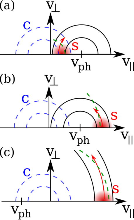
When quasilinear diffusion occurs according to Equation (3), particles diffuse in velocity space along curves of constant energy in the wave frame (i.e., the reference frame that moves with the speed $\omega_{k\mathrm{r}}/k_{\parallel}$ along $\mathbf{B}_{0}$). This diffusive flux of particles is locally tangent to semicircles centered on the parallel phase velocity $v_{\mathrm{ph}}\equiv\omega_{k\mathrm{r}}/k_{\parallel}$ (see also Figure 1), which satisfy the equation

At the same time, Equation (3) allows for diffusion only from higher phase-space densities to lower phase-space densities. Only waves and particles fulfilling the resonance condition

participate in the resonant wave–particle interaction due to the $\delta$-function in Equation (3).

Complementary to Equation (3), Kennel & Wong 1967 calculated the growth/damping rate of waves with $|\gamma_{k}|\ll|\omega_{k\mathrm{r}}|$ in quasilinear theory and found that the contribution of species $j$ to $\gamma_{k}$ is given by

where

$\varepsilon_{\mathrm{h}}$ denotes the Hermitian part of the dielectric tensor, and $f_{0j}$ is the background distribution function of species $j$.²² 2 For the following discussion, we focus on waves with $W_{k}>0$. The arguments are inverted for negative-energy waves. This effect is, however, not relevant for the parameter range explored in this study (Verscharen & Chandran 2013, cf.). The plasma frequency of species $j$ is defined by $\omega_{\mathrm{p}j}\equiv\sqrt{4\pi n_{0j}q_{j}^{2}/m_{j}}$. We assume that the background distribution functions $f_{0j}$ are represented by drifting Maxwellians,

where $w_{j}\equiv\sqrt{2k_{\mathrm{B}}T_{0j}/m_{j}}$ is the thermal speed of species $j$, $k_{\mathrm{B}}$ is the Boltzmann constant, and $T_{0j}$ is the equilibrium temperature of species $j$. The set of Equations (10) and (3) couple the evolution of the waves and particles in the presence of resonant wave–particle interactions and fulfill energy conservation (Kennel & Wong 1967; Chandran et al. 2010).

Figure 1 shows quasilinear diffusion paths for resonant strahl particles in velocity space. The relative alignment of the gradients of $f_{0j}$ in velocity space and the semicircles given by Equation (8) determines if the resonant particles lose or gain kinetic energy during the quasilinear diffusion process. In case (a), $0<U_{0\mathrm{s}}<v_{\mathrm{ph}}$, the resonant particles gain kinetic energy as they diffuse (i.e., their distance, $v_{\perp}^{2}+v_{\parallel}^{2}$, from the origin increases). They remove this energy from the resonant wave, which consequently decreases in amplitude. Therefore, case (a) represents a configuration that leads to wave damping. In case (b), $0<v_{\mathrm{ph}}<U_{0\mathrm{s}}$, the resonant particles lose kinetic energy as they diffuse and transfer this energy to the resonant wave, which consequently grows in amplitude. Therefore, case (b) represents a configuration that leads to wave instability. Case (c), in which $U_{0\mathrm{s}}>0$ and $v_{\mathrm{ph}}<0$, represents an additional configuration that leads to wave damping since the resonant particles gain kinetic energy during quasilinear diffusion.

We, therefore, conclude that

is a necessary condition in order for strahl electrons to lose kinetic energy through a wave–particle resonance. At this point, we limit ourselves to $\omega_{k\mathrm{r}}>0$ and $k_{\parallel}>0$ without loss of generality.³³ 3 Our arguments for instability also apply to a configuration in which $U_{0\mathrm{s}}<v_{\mathrm{ph}}<0$ (Verscharen & Chandran 2013; Verscharen et al. 2013a, see). If the strahl streams away from the Sun, the configuration $U_{0\mathrm{s}}<0$ corresponds to the case in which $\mathbf{B}_{0}\cdot\hat{\mathbf{e}}_{r}<0$, where $\hat{\mathbf{e}}_{r}$ is the radial unit vector in the solar rest frame.

The frequency $\omega_{k\mathrm{r}}$ is associated with the wavevector through the linear dispersion relation. Figure 2 shows two representative plots for the FM/W-wave dispersion relation (for details, see Section IV) with $\omega_{k\mathrm{r}}>0$ and $k_{\parallel}>0$. In addition, we plot the resonance condition in Equation (9) for $n=-1$ and $n=+1$. Resonant interactions only occur for waves and particles for which the line corresponding to the resonance condition intersects the plot of the dispersion relation. Figure 2 illustrates that strahl electrons with $v_{\parallel}>0$ only fulfill the resonance condition with FM/W waves with $\omega_{k\mathrm{r}}>0$ and $k_{\parallel}>0$ through resonance with $n\geq 0$. They cannot fulfill the resonance condition with these waves through resonances with $n\leq-1$ since $\omega_{k\mathrm{r}}<|\Omega_{\mathrm{e}}|$ for all $\mathbf{k}$ and $\Omega_{\mathrm{e}}<0$. We do not consider the $n=0$ strahl resonance since this resonance only excites instabilities when there is a bump-on-tail distribution (i.e., $\partial f_{j}/\partial v_{\parallel}>0$ at the resonance speed), which is not observed (see also Section VI.4). Moreover, instabilities driven via the $n=0$ strahl resonance are unable to account for the halo formation since they cause particles to diffuse only in $v_{\parallel}$ and not in $v_{\perp}$.

Although we will allow for oblique modes, we still limit ourselves to $k_{\perp}\rho_{\mathrm{e}}\ll 1$ to avoid cyclotron damping by the core, where $\rho_{\mathrm{e}}\equiv w_{\mathrm{e}}/|\Omega_{\mathrm{e}}|$, a point that we discuss further in Section IV.1 below.

When $k_{\perp}\rho_{\mathrm{e}}\ll 1$ and $n>0$, the only non-negligible term in Equation (5) is $E_{k,\mathrm{l}}e^{-i\phi}J_{n-1}(x_{j})$ which, moreover, is nonzero only when $n=+1$, because $J_{\nu}(x_{j})\rightarrow 0$ for $x_{j}\rightarrow 0$ for all $\nu\neq 0$. Therefore, in order for electrons to undergo an $n>0$ resonance with FM/W waves with $k_{\perp}\rho_{\mathrm{e}}\ll 1$, the FM/W waves must have a left-circularly polarized component (i.e., $E_{k,\mathrm{l}}\neq 0$). This requirement rules out the parallel-propagating FM/W wave, which is purely right-circularly polarized (i.e., $E_{k,\mathrm{l}}=0$), forcing us to consider obliquely propagating FM/W waves.⁴⁴ 4 The only left-circularly polarized parallel-propagating normal mode is the Alfvén/ion-cyclotron mode. This mode, however, has low frequencies ($\lesssim\Omega_{\mathrm{p}}$) compared to $|\Omega_{\mathrm{e}}|$. At these frequencies and under typical solar-wind conditions, thermal protons fulfill the resonance condition in Equation (9), so that the mode is prone to strong proton-cyclotron damping.

Figure 1 (b) shows a case that satisfies all of these requirements for the instability of the oblique FM/W wave. The diffusing particles increase in $v_{\perp}$ and (slightly) decrease in $v_{\parallel}$. These particles are the seed for the halo population. However, scattering by the initially excited FM/W waves does not fully describe the formation of the observed halo since it is restricted to particles in a certain range in $v_{\parallel}$ that fulfill the resonance condition. The scattered seed population, however, represents a strong deformation of the electron distribution function, which may eventually relax through secondary instabilities into a more symmetric halo about the electron core. A detailed study of the nonlinear evolution of the electron system is, however, beyond the scope of this work.

We assume that the instability drive by strahl electrons is most efficient at the center of the strahl distribution function, i.e., by particles with $v_{\parallel}=U_{0\mathrm{s}}$ and $v_{\perp}=0$. Through the $n=+1$ resonance, the oblique FM/W instability only occurs at frequencies of about

according to Equation (9).

We discuss the properties of the FM/W mode at different angles of propagation in the $\omega_{\mathrm{r}}$-$k_{\parallel}$ plane in Figure 3, where we show four solutions from the full dispersion relation of a hot electron–proton plasma. We use the linear Vlasov–Maxwell solver NHDS (Verscharen et al. 2013b; Verscharen & Chandran 2018, for details on the numerics, see).

In addition, we show Equation (15). The intersection between this line and a plot of the dispersion relation indicates a wavenumber and frequency at which the resonance condition between the wave and an electron with $v_{\parallel}=U_{0\mathrm{s}}$ is fulfilled. Since highly oblique modes cease to exist in plasmas with Maxwellian background distributions at large $\beta_{\mathrm{p}}\equiv 8\pi n_{0\mathrm{p}}T_{0\mathrm{p}}/B_{0}^{2}$ due to increasing Landau damping, we apply lower $\beta_{\mathrm{p}}$ for the highly oblique cases in Figure 3.⁵⁵ 5 We note that the lower $\beta_{\mathrm{p}}$-value used for the highly oblique solutions in Figure 3 is not representative for the solar wind at 1 au, but represents coronal conditions instead. We note that $k_{\perp}$ in the case with $\theta=89^{\circ}$ is by a factor $\tan\theta\sim 57$ greater than $k_{\parallel}$. The FM/W mode exists in two regimes in the wavenumber range in which Equation (15) can be fulfilled—i.e., where the line of the strahl resonance intersects with the corresponding plot of the dispersion relation. Regime 1 is the whistler regime in which the angle of propagation fulfills $0^{\circ}\leq\theta\lesssim 70^{\circ}$, and

where $d_{\mathrm{e}}\equiv v_{\mathrm{Ae}}/|\Omega_{\mathrm{e}}|$ is the electron inertial length. Equation (16) follows from the cold-plasma dispersion relation in a plasma with a single electron species under the assumption that $kd_{\mathrm{p}}\gg 1$, where $d_{\mathrm{p}}$ is the proton inertial length, and is approximately valid for small $\beta_{\mathrm{c}}$ and $\beta_{\mathrm{p}}$. The dispersion relation asymptotes toward $\sim|\Omega_{\mathrm{e}}|\cos\theta$ for large $k_{\parallel}$ provided that $\cos^{2}\theta\gtrsim m_{\mathrm{e}}/m_{\mathrm{p}}$. In the highly oblique limit (regime 2; i.e., $\cos^{2}\theta\lesssim m_{\mathrm{e}}/m_{\mathrm{p}}$), the wave propagates in the lower-hybrid regime. Its frequency asymptotes toward a frequency of order the lower-hybrid frequency,

as long as thermal corrections are small (Verdon et al. 2009).

To determine whether the oblique FM/W wave is unstable, we must consider not only the instability drive provided by the strahl, but also the possibility of damping by the core electrons. According to Equations (9) and (13), cyclotron damping by the core with $n=-1$ occurs at wavenumbers and frequencies that fulfill

Landau damping by the core with $n=0$ occurs at wavenumbers and frequencies that fulfill

Strahl driving with $n=+1$ occurs at wavenumbers and frequencies that fulfill Equation (15).

Figure 4 shows the plot of the dispersion relation from Equation (16), the strahl-resonance line from Equation (15), and the parameter space in which core Landau damping and core cyclotron damping act from Equations (18) and (19). For this plot, we have assumed that $w_{\mathrm{c}}\ll v_{\mathrm{Ae}}$. To a first approximation, the FM/W wave is unstable if there is a wavenumber range in which Equation (15) is fulfilled and Equations (18) and (19) are not fulfilled. The resonance line in Figure 4 represents the minimum $U_{0\mathrm{s}}$ for which strahl driving can occur in a wavenumber range in which neither core cyclotron damping nor core Landau damping acts. In order for the dispersion relation to intersect this resonance line within the white triangle, two conditions must be met: (1) $\beta_{\mathrm{e}}$ must be small (otherwise the dispersion relation will lie within the Landau-damped region – see Figure 4), and (2) $\theta$ must be $\simeq 60^{\circ}$. When these conditions are satisfied, the frequency of the resonant waves is given by

Furthermore, it follows from Equations (18) and (19) that the wavenumber of the resonant waves satisfies

where $k_{\mathrm{crit}}$ is the minimum wavenumber at which the green and blue regions in Figure 4 overlap; i.e., the minimum wavenumber at which both core Landau damping and core cyclotron damping can occur. Combining Equations (15), (20), and (21) leads to the instability criterion

For $\beta_{\mathrm{c}}\sim 1$, the dispersion relation lies below the Landau-damping threshold from $k_{\parallel}=0$ to $k_{\parallel}=k_{\mathrm{crit}}$. This situation is illustrated in Figure 5. We now determine the instability threshold in this regime by balancing the destabilizing effects of the strahl against the stabilizing effects of core Landau damping. Under these assumptions, the FM/W mode is unstable if there is a wavenumber range in which

Using Equation (11), we derive the instability criterion in Appendix A. We find that the FM/W mode is unstable if

for the $\beta_{\mathrm{c}}\sim 1$ case. The minimum of the right-hand side of Equation (24) suggests that the lowest threshold occurs for $\cos\theta=-1+\sqrt{2}$, i.e., for $\theta\approx 65.6^{\circ}$. The transition between the low-$\beta_{\mathrm{c}}$ case and the $\beta_{\mathrm{c}}\sim 1$ case occurs when $w_{\mathrm{c}}$ is large enough that the inequality in Equation (19) encompasses the entire plot of the dispersion relation. By combining Equation (16) for $\theta=60^{\circ}$ and Equation (19), we find that this transition occurs when

We compare our analytical thresholds from Equations (22) and (24) with numerical solutions of the hot-plasma dispersion relation from our NHDS code in Figure 6.

Our analytical instability thresholds agree well with our numerical solutions. The transition between the low-$\beta_{\mathrm{c}}$ case and the $\beta_{\mathrm{c}}\sim 1$ case occurs at $w_{\mathrm{c}}\approx 0.2v_{\mathrm{Ae}}$, which is slightly below our analytical finding in Equation (25). We attribute this difference to inaccuracies based on our assumption of a discrete onset of Landau damping as soon as $\omega_{k\mathrm{r}}\leq k_{\parallel}w_{\mathrm{c}}$.

The parallel-propagating FM/W wave is purely right-handed in polarization (i.e., $E_{k,\mathrm{l}}=E_{kz}=0$). Equation (5) for $k_{\perp}=0$, therefore, requires that the only contributing resonant interaction is the cyclotron resonance with $n=-1$. The resonant particles driving this instability must move in the opposite direction along the magnetic field as the wave (i.e., $v_{\parallel}<0$ in our convention) in order to fulfill the resonance condition, Equation (9). This property characterizes the halo rather than the strahl. If unstable, this mode corresponds to the whistler heat-flux instability (Gary & Feldman 1977; Gary et al. 1999; Wilson et al. 2009; Wilson et al. 2013; Shaaban et al. 2018a). The diffusion paths for this instability are shown in Figure 8 (Shaaban et al. 2019, see also).

The resonant particles diffuse toward smaller values of $v_{\perp}$ and form a tail-like structure in the distribution. This behavior does not agree with the scenario that strahl scattering forms the halo distribution function as discussed in Section II. For these reasons, we exclude the parallel whistler heat-flux instability as a candidate for a plasma instability that scatters the strahl into the halo. This instability can, however, be relevant for the regulation of the halo heat flux in the solar wind. Its threshold then also depends on the halo anisotropy (Shaaban et al. 2018b). We note that a reduction of $U_{0\mathrm{c}}$ can lead to an indirect reduction of $U_{0\mathrm{s}}$ by the fulfillment of quasi-neutrality according to Equation (2). This indirect effect is also relevant for the ion-acoustic heat-flux instability and for the KAW heat-flux instability. Evidence for the whistler heat-flux instability was found in measurements of solar-wind core and halo electrons (Tong et al. 2019).

In the limit $\cos^{2}\theta<m_{\mathrm{e}}/m_{\mathrm{p}}$, the FM/W-mode branch corresponds to the lower-hybrid mode as shown in Section IV.1. The fan instability of the lower-hybrid mode is driven by the $n=+1$ resonance of strahl electrons like the oblique FM/W instability (Omelchenko et al. 1994; Shevchenko & Galinsky 2010). It scatters particles about the parallel phase speed of the lower-hybrid wave, $v_{\mathrm{ph}}=\omega_{\mathrm{LH}}/k_{\parallel}$, and is, thus, capable of scattering strahl electrons into the halo. The highly oblique lower-hybrid mode has a strong electrostatic component and relatively low frequencies compared to the moderate-$\theta$ FM/W mode. Therefore, it is prone to strong core Landau damping if $w_{\mathrm{c}}$ is large enough that the core provides a significant number of electrons at $v_{\parallel}\approx v_{\mathrm{ph}}$. In this case, the resonance speed for Landau-resonant core electrons lies deep within the core distribution function. With increasing $w_{\mathrm{c}}$, the phase speed of the lower-hybrid wave increases slightly due to thermal corrections to its dispersion relation. This effect can overcompensate the increasing number of Landau-resonant core electrons at the strahl resonance speed. However, the growth rate of the highly oblique lower-hybrid mode is still less than the growth rate of the oblique FM/W instability by about two orders of magnitude under typical solar-wind conditions. As $U_{0\mathrm{s}}$ increases, $|U_{0\mathrm{c}}|$ must increase so that the parallel current vanishes as per Equation (2). In cases with very low $\beta_{\mathrm{c}}$, the lower-hybrid fan instability is a good candidate for self-induced strahl scattering. This situation is illustrated in Figure 9.

The instability is related to the oblique FM/W instability since it is driven by the same resonance effect and transitions into the oblique FM/W mode for smaller $\theta$. We note that some authors use a broader definition of the term fan instabilities for all instabilities driven by an $n=+1$ resonance (Krafft & Volokitin 2003, e.g., ).

The ion-acoustic heat-flux instability (Gary 1978) has a comparable instability threshold to the threshold of the oblique FM/W instability under certain conditions. However, this instability acts on particles with $v_{\parallel}\approx v_{\mathrm{ph}}$. The parallel phase speed of the ion-acoustic mode is much less than both $w_{\mathrm{c}}$ and the typical strahl speed in the solar wind. Therefore, it is more likely that this instability is driven by the core drift, which is directed in the opposite direction of the strahl speed according to Equation (2). For this case, we illustrate the quasilinear diffusion of particles under the action of the ion-acoustic instability in Figure 10. The ion-acoustic heat-flux instability is driven by the Landau resonance of the core electrons, which leads to a diffusion of core electrons at $v_{\parallel}=v_{\mathrm{ph}}$ toward smaller $|v_{\parallel}|$. This instability is not a candidate to explain strahl scattering into the halo since it does not increase $v_{\perp}$ of strahl electrons. We also note that large $T_{0\mathrm{c}}\gg T_{0\mathrm{p}}$ are required in order to increase $v_{\mathrm{ph}}$ of the ion-acoustic mode and to avoid proton Landau damping, which would otherwise efficiently suppress this instability. The maximum growth rate of the ion-acoustic heat-flux instability occurs in parallel propagation.

The same instability mechanism is responsible for the kinetic-Alfvén-wave (KAW) heat-flux instability (Gary et al. 1975a). In the parameter range explored by Gary et al. 1975a, the KAW heat-flux instability requires low $\beta_{\mathrm{c}}\lesssim 10^{-3}$ to have the lowest threshold of all electron-drift driven instabilities. It propagates at very large angles $\theta$ with respect to $\mathbf{B}_{0}$. The nonzero $E_{kz}$ of the KAW allows for the electron core to drive the mode unstable through the Landau resonance as in the case of the ion-acoustic heat-flux instability. Likewise, this instability does not scatter strahl particles into the halo.

The electrostatic electron-beam instability (Gary 1978) is a low-$\beta_{\mathrm{c}}$ instability that propagates into the direction of the strahl and has maximum growth parallel to $\mathbf{B}_{0}$. Its typical phase speed is $v_{\mathrm{ph}}\lesssim U_{0\mathrm{s}}$. For $\beta_{\mathrm{c}}\lesssim 0.1$, it has lower thresholds than the other instabilities, as long as the strahl forms a bump-on-tail configuration rather than a shoulder of the distribution while all other parameters are kept at representative solar-wind values. It is driven by the Landau resonance of the strahl electrons. We illustrate this instability in Figure 11.

The Landau-resonant diffusion of strahl electrons leads to an excitation of this instability only if the diffusion paths down the gradients of the strahl distribution function are directed to lower kinetic energies. For this reason, $U_{0\mathrm{s}}$ has to be slightly greater than $v_{\mathrm{ph}}$ as illustrated in Figure 11. This instability only reduces $v_{\parallel}$ and does not increase $v_{\perp}$ of the resonant strahl electrons and is thus not a candidate mechanism to scatter strahl electrons into the halo. We also note that, if this instability were to operate in the solar wind, it would lead to a quasilinear flattening of the electron distribution function in at least some narrow range of parallel velocities near the strahl velocity. However, the measured electron distribution functions are strongly decreasing functions of $v_{\parallel}$ near the strahl velocity (Pilipp et al. 1987a; Marsch 2006).

References

- Alexandrova et al. (2012) Alexandrova, O., Lacombe, C., Mangeney, A., Grappin, R., & Maksimovic, M. 2012, ApJ, 760, 121
- Alexandrova et al. (2009) Alexandrova, O., Saur, J., Lacombe, C., et al. 2009, Phys. Rev. Lett., 103, 165003
- Bale et al. (2013) Bale, S. D., Pulupa, M., Salem, C., Chen, C. H. K., & Quataert, E. 2013, ApJ, 769, L22
- Bender & Orszag (1999) Bender, C. M., & Orszag, S. A. 1999, Advanced Mathematical Methods for Scientists and Engineers I (New York, USA: Springer)
- Chandran et al. (2010) Chandran, B. D. G., Pongkitiwanichakul, P., Isenberg, P. A., et al. 2010, ApJ, 722, 710
- Chen et al. (2012) Chen, C. H. K., Salem, C. S., Bonnell, J. W., Mozer, F. S., & Bale, S. D. 2012, Phys. Rev. Lett., 109, 035001
- Detering et al. (2005) Detering, F., Rozmus, W., Brantov, A., et al. 2005, Phys. Plasmas, 12, 012321
- Feldman et al. (1976) Feldman, W. C., Asbridge, J. R., Bame, S. J., Gary, S. P., & Montgomery, M. D. 1976, J. Geophys. Res., 81, 2377
- Feldman et al. (1975) Feldman, W. C., Asbridge, J. R., Bame, S. J., Montgomery, M. D., & Gary, S. P. 1975, J. Geophys. Res., 80, 4181
- Fitzenreiter et al. (1998) Fitzenreiter, R. J., Ogilvie, K. W., Chornay, D. J., & Keller, J. 1998, Geophys. Res. Lett., 25, 249
- Gary (1978) Gary, S. P. 1978, J. Plasma Phys., 20, 47
- Gary (1979) —. 1979, J. Plasma Phys., 21, 361
- Gary & Feldman (1977) Gary, S. P., & Feldman, W. C. 1977, J. Geophys. Res., 82, 1087
- Gary et al. (1975a) Gary, S. P., Feldman, W. C., Forslund, D. W., & Montgomery, M. D. 1975a, Geophys. Res. Lett., 2, 79
- Gary et al. (1975b) —. 1975b, J. Geophys. Res., 80, 4197
- Gary & Li (2000) Gary, S. P., & Li, H. 2000, ApJ, 529, 1131
- Gary & Saito (2007) Gary, S. P., & Saito, S. 2007, Geophys. Res. Lett., 34, 14111
- Gary et al. (1994) Gary, S. P., Scime, E. E., Phillips, J. L., & Feldman, W. C. 1994, J. Geophys. Res., 99, 23391
- Gary et al. (1999) Gary, S. P., Skoug, R. M., & Daughton, W. 1999, Phys. Plasmas, 6, 2607
- Gosling et al. (2001) Gosling, J. T., Skoug, R. M., & Feldman, W. C. 2001, Geophys. Res. Lett., 28, 4155
- Graham et al. (2017) Graham, G. A., Rae, I. J., Owen, C. J., et al. 2017, J. Geophys. Res., 122, 3858
- Gurgiolo & Goldstein (2017) Gurgiolo, C., & Goldstein, M. L. 2017, Annales Geophysicae, 35, 71
- Hammond et al. (1996) Hammond, C. M., Feldman, W. C., McComas, D. J., Phillips, J. L., & Forsyth, R. J. 1996, A&A, 316, 350
- He et al. (2012) He, J., Tu, C., Marsch, E., & Yao, S. 2012, ApJ, 745, L8
- Hollweg (1974) Hollweg, J. V. 1974, J. Geophys. Res., 79, 3845
- Horaites et al. (2018) Horaites, K., Astfalk, P., Boldyrev, S., & Jenko, F. 2018, MNRAS, 480, 1499
- Kennel & Wong (1967) Kennel, C. F., & Wong, H. V. 1967, J. Plasma Phys., 1, 75
- Krafft & Volokitin (2003) Krafft, C., & Volokitin, A. 2003, Ann. Geophys., 21, 1393
- Krafft & Volokitin (2006) —. 2006, Phys. Plasmas, 13, 122301
- Krafft et al. (2005) Krafft, C., Volokitin, A., & Zaslavsky, A. 2005, Phys. Plasmas, 12, 112309
- Lakhina (1977) Lakhina, G. S. 1977, Sol. Phys., 52, 153
- Lakhina (1979) —. 1979, Ap&SS, 63, 511
- Landi & Pantellini (2003) Landi, S., & Pantellini, F. 2003, A&A, 400, 769
- Lazar et al. (2013) Lazar, M., Poedts, S., & Michno, M. J. 2013, A&A, 554, A64
- Lazar et al. (2011) Lazar, M., Poedts, S., & Schlickeiser, R. 2011, Monthly Not. Royal Astron. Soc., 410, 663
- Lie-Svendsen et al. (1997) Lie-Svendsen, Ø., Hansteen, V. H., & Leer, E. 1997, J. Geophys. Res., 102, 4701
- Lin (1998) Lin, R. P. 1998, Space Sci. Rev., 86, 61
- Lin et al. (1995) Lin, R. P., Anderson, K. A., Ashford, S., et al. 1995, Space Sci. Rev., 71, 125
- Maksimovic et al. (2000) Maksimovic, M., Gary, S. P., & Skoug, R. M. 2000, J. Geophys. Res., 105, 18337
- Maksimovic et al. (1997) Maksimovic, M., Pierrard, V., & Riley, P. 1997, Geophys. Res. Lett., 24, 1151
- Maksimovic et al. (2005) Maksimovic, M., Zouganelis, I., Chaufray, J.-Y., et al. 2005, J. Geophys. Res., 110, 9104
- Marsch (2006) Marsch, E. 2006, Living Rev. Solar Phys., 3, 1
- Omelchenko et al. (1994) Omelchenko, Y. A., Shapiro, V. D., Shevchenko, V. I., Ashour-Abdalla, M., & Schriver, D. 1994, J. Geophys. Res., 99, 5965
- Owens et al. (2008) Owens, M. J., Crooker, N. U., & Schwadron, N. A. 2008, J. Geophys. Res., 113, A11104
- Pagel et al. (2005) Pagel, C., Crooker, N. U., Larson, D. E., Kahler, S. W., & Owens, M. J. 2005, J. Geophys. Res., 110, 1103
- Pavan et al. (2013) Pavan, J., Viñas, A. F., Yoon, P. H., Ziebell, L. F., & Gaelzer, R. 2013, ApJ, 769, L30
- Phillips & Gosling (1990) Phillips, J. L., & Gosling, J. T. 1990, J. Geophys. Res., 95, 4217
- Pilipp et al. (1987a) Pilipp, W. G., Muehlhaeuser, K.-H., Miggenrieder, H., Montgomery, M. D., & Rosenbauer, H. 1987a, J. Geophys. Res., 92, 1075
- Pilipp et al. (1987b) Pilipp, W. G., Muehlhaeuser, K.-H., Miggenrieder, H., Rosenbauer, H., & Schwenn, R. 1987b, J. Geophys. Res., 92, 1103
- Pongkitiwanichakul & Chandran (2014) Pongkitiwanichakul, P., & Chandran, B. D. G. 2014, ApJ, 796, 45
- Pulupa et al. (2014) Pulupa, M. P., Bale, S. D., Salem, C., & Horaites, K. 2014, J. Geophys. Res., 119, 647
- Ramani & Laval (1978) Ramani, A., & Laval, G. 1978, Phys. Fluids, 21, 980
- Roberg-Clark et al. (2019) Roberg-Clark, G. T., Agapitov, O. V., Drake, J. F., & Swisdak, M. M. 2019, arXiv e-prints, arXiv:1908.06481
- Roberg-Clark et al. (2016) Roberg-Clark, G. T., Drake, J. F., Reynolds, C. S., & Swisdak, M. 2016, ApJ, 830, L9
- Roberg-Clark et al. (2018) Roberg-Clark, G. T., Drake, J. F., Swisdak, M., & Reynolds, C. S. 2018, ApJ, 867, 154
- Rosenbauer et al. (1977) Rosenbauer, H., Schwenn, R., Marsch, E., et al. 1977, J. Geophysics, 42, 561
- Sahraoui et al. (2012) Sahraoui, F., Belmont, G., & Goldstein, M. L. 2012, ApJ, 748, 100
- Sahraoui et al. (2010) Sahraoui, F., Goldstein, M. L., Belmont, G., Canu, P., & Rezeau, L. 2010, Phys. Rev. Lett., 105, 131101
- Salem et al. (2003a) Salem, C., Hoang, S., Issautier, K., Maksimovic, M., & Perche, C. 2003a, Adv. Space Res., 32, 491
- Salem et al. (2003b) Salem, C., Hubert, D., Lacombe, C., et al. 2003b, ApJ, 585, 1147
- Salem et al. (2012) Salem, C. S., Howes, G. G., Sundkvist, D., et al. 2012, ApJ, 745, L9
- Scime et al. (1999) Scime, E. E., Badeau, Jr., A. E., & Littleton, J. E. 1999, Geophys. Res. Lett., 26, 2129
- Scudder & Olbert (1979a) Scudder, J. D., & Olbert, S. 1979a, J. Geophys. Res., 84, 2755
- Scudder & Olbert (1979b) —. 1979b, J. Geophys. Res., 84, 6603
- Shaaban et al. (2018a) Shaaban, S. M., Lazar, M., & Poedts, S. 2018a, MNRAS, 480, 310
- Shaaban et al. (2018b) Shaaban, S. M., Lazar, M., Yoon, P. H., & Poedts, S. 2018b, Phys. Plasmas, 25, 082105
- Shaaban et al. (2019) Shaaban, S. M., Lazar, M., Yoon, P. H., Poedts, S., & López, R. A. 2019, MNRAS, 486, 4498
- Shevchenko & Galinsky (2010) Shevchenko, V. I., & Galinsky, V. L. 2010, Nonlinear Processes in Geophysics, 17, 593
- Stix (1992) Stix, T. H. 1992, Waves in plasmas (New York, USA: American Institute of Physics)
- Tong et al. (2019) Tong, Y., Vasko, I. Y., Pulupa, M., et al. 2019, ApJ, 870, L6
- Štverák et al. (2009) Štverák, Š., Maksimovic, M., Trávníček, P. M., et al. 2009, J. Geophys. Res., 114, 5104
- Štverák et al. (2008) Štverák, Š., Trávníček, P., Maksimovic, M., et al. 2008, Journal of Geophysical Research (Space Physics), 113, 3103
- Vasko et al. (2019) Vasko, I. Y., Krasnoselskikh, V., Tong, Y., et al. 2019, ApJ, 871, L29
- Verdon et al. (2009) Verdon, A. L., Cairns, I. H., Melrose, D. B., & Robinson, P. A. 2009, in IAU Symposium, Vol. 257, IAU Symposium, ed. N. Gopalswamy & D. F. Webb, 569–573
- Verscharen et al. (2013a) Verscharen, D., Bourouaine, S., & Chandran, B. D. G. 2013a, ApJ, 773, 163
- Verscharen et al. (2013b) Verscharen, D., Bourouaine, S., Chandran, B. D. G., & Maruca, B. A. 2013b, ApJ, 773, 8
- Verscharen & Chandran (2013) Verscharen, D., & Chandran, B. D. G. 2013, ApJ, 764, 88
- Verscharen & Chandran (2018) —. 2018, Res. Notes AAS, 2, 13
- Verscharen et al. (2018) Verscharen, D., Klein, K. G., Chandran, B. D. G., et al. 2018, J. Plasma Phys., 84, 905840403
- Verscharen et al. (2019) Verscharen, D., Klein, K. G., & Maruca, B. A. 2019, Living Rev. Solar Phys., accepted
- Vocks & Mann (2003) Vocks, C., & Mann, G. 2003, ApJ, 593, 1134
- Watson (1922) Watson, G. N. 1922, A Treatise on the Theory of Bessel Functions (New York, USA: Cambridge University Press)
- Wilson et al. (2009) Wilson, L. B., I., Cattell, C. A., Kellogg, P. J., et al. 2009, J. Geophys. Res., 114, A10106
- Wilson et al. (2018) Wilson, Lynn B., I., Stevens, M. L., Kasper, J. C., et al. 2018, ApJS, 236, 41
- Wilson et al. (2013) Wilson, L. B., Koval, A., Szabo, A., et al. 2013, J. Geophys. Res., 118, 5