From Caesar Cipher to Unsupervised Learning:
A New Method for Classifier Parameter Estimation

The Caesar cipher, also known as shift cipher, is one of the simplest forms of encryption. It has been first used by Julius Caesar, the well-known Roman general who led to the rise of the Roman Empire. And the encryption technique was named after him. Caesar Cipher is a substitution cipher where each letter in the plain text, or the original message, is replaced with another letter corresponding to a certain number of letters up or down in the alphabet. For example, in Figure 1, the message in the plain text is “THE QUICK BROWN FOX JUMPS OVER THE LAZY DOG”. With a shift of 3 letters up, the encrypted message becomes “QEB NRFZH YOLTK CLU GRJMP LSBO IXWV ALD”.

To decrypt Caesar Cipher with unknown shift, we need three steps: 1) acquiring standard English statistics as a “prior”; 2) calculating the same statistics of the encrypted message, and 3) matching the two statistics with a trial-and-error scheme to recover the shift. Here we assume that the encrypted message is large enough that the number of letters has statistical significance. The process is illustrated in Figure 2 and explained in details as follows Cipher 2009:

Step 1: Prior standard English statistics To discover the correspondence between the encrypted letters and standard English letters, we first need to know precisely how the encrypted letters look like in the standard alphabet. To this end, for example, one can take a large bulk of standard English corpus (e.g. newspapers) and calculate the frequency or histogram of each of 26 English letters, as shown in lower part of the Figure 2.

Step 2: Encrypted message statistics Similarly, we can determine the same statistics on our encrypted original message. This can be accomplished by counting the frequency of each letters in the encrypted message. We may give the histogram that looks like the one on the upper part of Figure 2 (after a shift).

Step 3: Matching the two statistics With the two histogram charts side by side, one can easily try out in a brute-force way all of 25 shifts and find the best match, as shown in Figure 2. After determining the shift, one can obtain the shifted alphabet and recover the original message.

Our unsupervised learning problem here is formulated in the simplest setting of binary classification where no input-output pairs are needed in the classifier training. The input $\mathcal{X}=(\mathbf{x_{1}},\dots,\mathbf{x_{T}})$ is a sequence of 2-dimensional vectors, where $\mathbf{x_{t}}=(x_{t}^{a},x_{t}^{b})\in\mathbb{R}^{2\times 1}$ is a 2-dimensional vector. The ground-truth labels $\mathcal{Y}=(y_{1},\dotsm y_{T})$ are the corresponding sequence, where each $y_{t}$ denotes the class that $x_{t}$ corresponds to. Note that the ground-truth labels are not used in the training. Here, analog to Caesar Cipher, the input sequence $\mathcal{X}$ acts as the encrypted message, and $\mathcal{Y}$ is the original message to recover.

Importantly, as any original English message is subject to English language rules, we also ask that $y_{t}$ be subject to a given “rule”. In this context, we call this rule as “language model” in the form of N-gram, i.e. the statistics of $y_{t}\sim p(y_{N}|y_{N-1},\dots,y_{1})$. In case of $N=1$, the language model reduces to the basic frequency distribution, i.e. Unigram, just like the statistics used in the example of Caesar Cipher. In case of $N>1$, the language model describes the sequential pattern by predicting the next letter in the form of a $(N-1)$-th order Markov model, e.g. $N=2$ the Bigram model. We will formulate unsupervised learning in detail assuming the Unigram model in this section, and walk through the Bigram case in Section V.

Our problem here is very similar to that of decryption of Caesar Cipher; i.e. given only the N-gram statistics (analogous to the Prior standard English statistics) and a sequence $(\mathbf{x_{1}},\dots,\mathbf{x_{T}})$, which is analogous to the original message) as the input, we desire to predict the true label sequence $(y_{1},\dotsm y_{T})$, which is analogous to the decrypted message).

Since the problem discussed here for pedagogical purposes is binary classification, we use the most common model, the log-linear model, as our classifier. In the log-linear model, the output of the classifier is a posterior probability. Recalling that the input is two-dimensional $\mathbf{x_{t}}=(x_{t}^{a},x_{t}^{b})$, we define the model that has two learnable parameters denoted as $\theta=\{w^{a},w^{b}\}$:

where $\gamma$ is a constant (e.g. we fix $\gamma=10$ in our experiments described in Section VI). These formulas calculate the probability of producing $y_{t}$ when receiving input $\mathbf{x_{t}}$. For example, if $p_{\theta,t}(0)\geq 0.5$, we predict label $\bar{y_{t}}=0$; otherwise we predict label $\bar{y_{t}}=1$. Note that from Eqn.(1), we always have $p_{\theta,t}(0)+p_{\theta,t}(1)=1$.

We approach the binary classification problem with unsupervised learning in three steps, analogous to decrypting Caesar Cipher described in Section III-B. The corresponding three main steps are: 1) Determine language model statistics as the prior on labels $\mathcal{Y}$; 2) Calculate the statistics on the classifier output, and 3) Match the two statistics with which a cost function is determined. Next we carry out this procedure step-by-step to create the cost function.

Step 1: Prior language model statistics. Since the dataset we use is synthetic data, i.e. both $\mathcal{X}$ and $\mathcal{Y}$ are known, we can easily obtain the statistics of a Unigram language model by calculating the probabilities below with all $y_{t}\in\mathcal{Y}$ given in the dataset:

Note that $p_{0},p_{1}\geq 0$ are constants with $p_{0}+p_{1}=0$.

Step 2: Classifier output statistics. The classifier outputs from Eqn.(1) directly determine the probability of data being assigned with each label. The Unigram (or histogram) statistics can be easily calculated by

where $\mathbf{\overline{P_{LM}}}(\theta)$ stands for the estimated language model from classifier which is parameterized by $\theta$.

Step 3: Matching the two statistics. In the same spirit of decryption of Caesar Cipher, we need to compare and then match the two statistics $\mathbf{P_{LM}}$ and $\mathbf{\overline{P_{LM}}}(\theta)$ in order to find the best decipher. As suggested in (Chen et al. 2016), the difference between two distributions can be measured by Kullback-Leibler (KL) divergence. The KL divergence of the true prior distribution $\mathbf{{P_{LM}}}$ and the estimated distribution $\mathbf{\overline{P_{LM}}}$ is:

where the sign $\oslash$ denotes element-wise division. We minimize $D_{KL}$ in order to learn the model parameters $\theta$ to the effect that the estimated statistics become as close to the prior statistics as possible. Note that in $D_{KL}$ of Eqn. (4), the second term $\mathbf{P_{LM}},\ln{\mathbf{{P_{LM}}^{T}}},$ is a constant and can be ignored in optimization. Thus, our objective function to be minimized becomes:

In summary, we formulate our problem of unsupervised learning in this pedagogical example as an optimization problem of finding the best classifier parameters $\theta^{*}$ according to

However, for the objective function of Eqn.(5), it is not feasible to use SGD-based optimizer to solve the above minimization problem above. This is due to two reasons: the high cost of computing the gradient and the highly non-convex profile of the objective function with respect to the parameters.

High cost of computing the gradient. The SGD-based optimizers, such as AdaGrad (Duchi et al. 2012) and ADAM (Kingma & Ba 2014), require that the sum over training samples be outside of the logarithmic loss (Ferguson 1982). However, in the above loss function, the sum over samples $t$, i.e. $\frac{1}{T}\sum_{t=1}^{T}$, is inside the logarithmic loss ($\ln$). This makes a very large difference from traditional neural network error minimization problems solved by SGD. The special form of the objective function in Eqn. (5) prevents us from applying SGD to minimize the cost.

Highly non-convex profile. Even worse, the cost function is highly non-convex, and hard to converge to the optimum. Figure 3 illustrates this non-convex surface of the cost function $\mathcal{J}(\theta)$ in in Eqn. (5). To obtain this profile surface, we take two steps. First, we use both data $\mathcal{X}$ and true labels $\mathcal{Y}$ to find the global optimum $\theta^{0}=(w^{a0},w^{b0})$ (the red points in the figures) by solving the supervised learning problem

This is an ordinary maximum posterior optimization problem with the sum over training sameples lying outside of the logarithm. Hence we solve it by plain SGD and plot with red dot in Figure 3. In the second step, we plot the two-dimensional function around $w^{a0},w^{b0}$, i.e. $\mathcal{J}(w^{a0}+\lambda_{1},w^{b0}+\lambda_{2})$ with respect to $\lambda_{1},\lambda_{2}\in\mathbb{R}$. We can observe the surface of the cost function $\mathcal{J}(\theta)$ and find that it is highly non-convex. There are many local optimal solutions and there is a high barrier that makes it difficult for naive optimization algorithms to reach the global optimum.

To overcome the above two difficulties, we can transform the optimization problem for the cost function in Eqn. (5) into an equivalent one, called saddle point problem, where the cost function has a more desirable profile surface for gradient-based methods. One such technique is introduced in Section IV next.

Let us first introduce a lemma that will be used in the later description of the saddle point problem.

Examining Lemma 1, we find $\ln{u}$ on the left side of the equation is transformed into an maximum over a different variable $v$ of a formula where $u$ comes outside the logarithm. Thus, we use this Lemma to rewrite the logarithm part in the cost function in Eqn. (5):

Let us now define the new cost function $\mathcal{L}(\theta,V)$ to be the quantity inside the $\min\max$ in Equation 10 above:

where $V=\{v_{0},v_{1}\}$. With the use of matrix form $\mathbf{V}=\begin{bmatrix}v_{0},v_{1}\end{bmatrix}$, as well as Equations (2) and (24), we rewrite the new cost function into a matrix form (where $\odot$ stands for pairwise multiplication between two matrices):

Let us provide interpretation for the new cost function $\mathcal{L}(\theta,\mathbf{V})$ in Eqn. (12), contrasting the earlier form of $\mathcal{J}(\theta)$ in Eqn. (5). In the new form, parameter $\mathbf{V}$ is called dual variables, and the original parameters $\mathbf{\theta}$ are called primal variables. Minimization of $\mathcal{J}(\theta)$ over primal variables $\theta$ has been transformed to a min-max problem on $\mathcal{L}(\theta,\mathbf{V})$ over both primal variables $\theta$ and dual variables $\mathbf{V}$. The min-max problem in this new form is called saddle-point problem. Specifically, the saddle-point problem can be solved by seeking a point, which is not only the minimum point along primal domain ($\theta$) but also the maximum point along dual domain ($\mathbf{V}$). This point, denoted as $(\theta^{*},\mathbf{V}^{*})$, is called the saddle point for the domain of $(\theta,\mathbf{V})$ [2]. Importantly, we find that the sum over $t$ has been taken outside of logarithm. As a result, we can now apply SGD or its variation in learning the model.

We now draw the profile of cost function $\mathcal{L}(\theta,\mathbf{V})$ in Figure 4. Like the profile surface of $\mathcal{J}(\theta)$ in Section IV-C, we need to first get $\theta^{0}$ by solving the supervised problem $\theta^{0}=\arg\max_{\theta}\sum_{t=1}^{T}\ln{p_{t,\theta}(y_{t}|x_{t})}$. Then, we inference $V^{0}$ by

With the supervised optima $\theta^{0},\mathbf{V^{0}}$, we can plot the 3-D cost function surface around this optima. We randomly choose two direction $(\theta^{1}-\theta^{0})$ and $(\mathbf{V^{1}}-\mathbf{V^{0}})$, where $\theta^{1}$ and $\mathbf{V^{1}}$ are random vectors with same size of $\theta^{0}$ and $\mathbf{V^{0}}$. Then we plot on the 3-D space the point $(\lambda_{p},\lambda_{d},Z(\lambda_{p},\lambda_{d}))$, with $Z(\lambda_{p},\lambda_{d})=\mathcal{J}(\theta^{*}+\lambda_{p}(\theta_{1}-\theta^{0}),\mathbf{V^{0}}+\lambda_{d}(\mathbf{V_{1}}-\mathbf{V^{0}}))$. The Figure 4 shows the plotting results.

Comparing surface of original surface in Figure 3 with surface of transformed cost function in Figure 4, we can see that, after the primal-dual reformulation, the barrier in original cost function $\mathcal{J}(\theta)$ disappears. Thus the optimization become much easier on the new cost function.

In this section, we proceed to find the solution to the saddle-point problem in Eqn. (12).

To solve a min-max problem, our idea is to minimize $\mathcal{L}(\theta,\mathbf{V})$ with respect to $\theta$, while, at the same time, maximize $\mathcal{L}(\theta,\mathbf{V})$ with respect to $\mathbf{V}$. Specifically, we solve the min-max problem by stochastic gradient descent of $\mathcal{L}(\theta,\mathbf{V})$ over $\theta$ while by stochastic accent of $\mathcal{L}(\theta,\mathbf{V})$ over $\mathbf{V}$ with following update equations:

The updates happens at time $\tau$. And $\mu_{\theta},\mu_{V}>0$ are learning rate for primal variables and dual variables, respectively. Note that we update two of primal and dual variables in a synchronized manor.

Now we derive the close form of $\frac{\partial\mathcal{L}}{\partial\mathbf{\theta}}$ and $\frac{\partial\mathcal{L}}{\partial\mathbf{V}}$. First, for $\frac{\partial\mathcal{L}}{\partial\mathbf{\theta}}$, from Eqn. (12), we take partial derivative:

where the term $\frac{\partial\mathbf{\overline{P_{LM}}}(\theta)}{\partial\mathbf{\theta}}$ in above can be decomposed and calculated in element-wise. Recall that $\mathbf{P_{LM}}=[p_{0},p_{1}]$ is constant, $\mathbf{\overline{P_{LM}}}(\theta)=[\frac{1}{T}\sum_{t=1}^{T}p_{\theta,t}(0),~~\frac{1}{T}\sum_{t=1}^{T}p_{\theta,t}(1)]^{T}$ and $\mathbf{\theta}=[w^{a},w^{b}]^{T}$. From matrix derivative rules we know:

where $p_{t,\theta}(0)$ and $p_{t,\theta}(1)$ are defined in Eqn. (1) being log-linear classifier model for classes $0$ and $1$, respectively. The four derivatives in Eqn. (16) can be calculated from definition in Eqn. (1). For example:

In above derivation, $\sigma(\cdot)$ indicate sigmoid function that $\sigma(a)=\frac{1}{1+e^{-a}}$. Note that we use the equation $\frac{\partial\sigma(a)}{\partial a}=\sigma(a)(1-\sigma(a))$ in above derivation. Similarly, we can get all the derivatives in matrix of 16 as:

Then we substitute all derivative terms in Eqn. (16) using (18):

Thus we get the final close form of $\frac{\partial\mathcal{L}}{\partial\mathbf{\theta}}$:

Then for $\frac{\partial\mathcal{L}}{\partial\mathbf{V}}$, recall that $\mathbf{V}=[v_{0},v_{1}]$. Simply use matrix derivative rules and we can get:

For mini-batch updates, we simply replace the sum over total data $T$ with sum over the mini-batch data $B=(\mathbf{x_{s}},…,\mathbf{x_{s+N-1}})$. For each update, a sequence of data with size $N$ is randomly taken from $\mathcal{X}$ as a mini-batch. Then we use Formula (14) to update both primal and dual variable with close form (20) and (21). Repeating this process until convergence. We describe the this process with mini-batch gradient in Algorithm 1.

However, we found the language model of Unigram is too weak. It does not capture the sequence structure which is important information for unsupervised classification. As in Chen et al. 2016, the sequence prior of output labels is a important structure to employ in unsupervised problems, especially when the order is high. However, the Unigram language model does not capture such structure.

However, the experiment results turns out to be unsatisfied. The average classification error rate is $30.8\%$, which is just about the error rate of majority guess. The model constantly predicts class with label 1, regardless of the input data. In experiment we conduct the experiments on the binary classification task with the dataset we created for $(\mathcal{X},\mathcal{Y})$.

Next, we will walk through this problem by using Bigram language model, the simplest language model with sequence prior statistics. The main procedure of the derivation is the same with Unigram we just did in previous sections. So it can be easier for readers to apply to Bigram case, in spite of more mathematics will be involved.

In Bigram case, the problem formulation and approach is the same as Unigram case that we also use model for classifier as in formula 1. except using Bigram language models. Here below are the three main steps accordingly.

Step 1: Prior language model statistics (Bigram) We will create synthetic data with arbitrary given language model. First, we create output labels $\mathcal{Y}=(y_{1},y_{2},\dots,y_{T})$ from a 1st-order Markov model that is based on a given transition probability:

$p(y_{t}|y_{t-1})$ denotes conditional probability of the transition between adjacent labels $y_{t-1}$ to $y_{t}$, which is given in transition matrix $\mathbf{P_{Trans}}$. Then, the language model $\mathbf{P_{LM}}$ can be calculated from the transition matrix:

$\mathbf{p_{st}}$ denotes the steady state vector of transition $\mathbf{P_{Trans}}$. The creation of data, as well as connection between language model and transition matrix will be explained in detail in experiment section VII.

Step 2: Classifier output statistics (Bigram) Due to first order dependency, the probability of data being assigned with each label by the classifier in Eqn. (1) can be calculated by:

Step 3: Matching the two statistics As with Unigram, we still use KL-divergence to measure the difference, and obtain cost function :

where the notation $\left\langle\mathbf{A},\mathbf{B}\right\rangle=\sum_{i}\sum_{j}a_{ij}b_{ij}$ stands for the inner product of two matrices $\mathbf{A}$ and $\mathbf{B}$, specifically, sum of the products of the corresponding components of two matrices. Thus, we formulate our problem as an optimization problem finding the best classifier parameters $\theta^{*}$:

We again observe the sum inside logarithm. With using Lemma 1, we can transform this problem to its equivalent saddle-point problem:

As in the case of Unigram, we define the new cost:

$\theta$ is called primal variables, and $\mathbf{V}$ is called dual variables. Thus, the minimization problem of $\mathcal{J}(\theta)$ over primal variables $\theta$ is transformed to an equivalent saddle-point problem of $\mathcal{L}(\theta,\mathbf{V})$, and the sum over $t$ has been taken outside of logarithm. In other words, the optimal solution $(\theta^{*},\mathbf{V}^{*})$ to $\mathcal{L}(\theta,\mathbf{V})$ is called the saddle point [2], which is relative minimum along primal domain $\theta$ while is a relative maximum along dual domain $\mathbf{V}$.

As in the Unigram case, we also visualize the profile surface of cost function $\mathcal{L}(\theta,\mathbf{V})$ in Figure 5. Again, we need to first get $\theta^{0}$ by solving the supervised problem $\theta^{0}=\arg\max_{\theta}\sum_{t=1}^{T}\ln{p_{t,\theta}(y_{t}|x_{t})}$, and inference $V^{0}$ using

Using the same method, we first randomly choose two direction $(\theta^{1}-\theta^{0})$ and $(\mathbf{V^{1}}-\mathbf{V^{0}})$, where $\theta^{1}$ and $\mathbf{V^{1}}$ are random vectors with same size of $\theta^{0}$ and $\mathbf{V^{0}}$. Then we plot on the 3-D space the point $(\lambda_{p},\lambda_{d},Z(\lambda_{p},\lambda_{d}))$, with $Z(\lambda_{p},\lambda_{d})=\mathcal{J}(\theta^{*}+\lambda_{p}(\theta_{1}-\theta^{0}),\mathbf{V^{0}}+\lambda_{d}(\mathbf{V_{1}}-\mathbf{V^{0}}))$. The Figure 5 shows the plotting results.

Similarly, we solve the min-max problem by stochastic gradient descent of $\mathcal{L}(\theta,V)$ over $\theta$ while by stochastic accent of $\mathcal{L}(\theta,V)$ over $V$ with the same update equations:

The updates happens at time $\tau$. And $\mu_{\theta},\mu_{V}>0$ are learning rate for primal variables and dual variables, respectively. Note that we update two of primal and dual variables in a synchronized manor.

By using Formula (19), we calculate ${\partial\mathcal{L}}/{\partial\mathbf{\theta}}$ and ${\partial\mathcal{L}/}{\partial\mathbf{V}}$ similar as the Unigram Case:

As Unigram, we also use mini-batch to calculate each update during training in the Bigram case. It is the same as the Unigram case with mini-batch gradient in Algorithm 1.

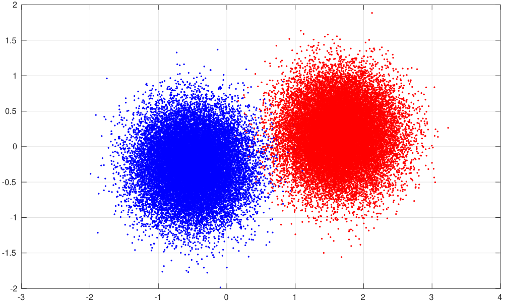
Data Generation We first create synthetic data with Unigram language model, where the data points and associated labels subject to a given Unigram language model, such as:

That is 69.2% of labels “0” and 30.8% of label “1” in $\mathcal{Y}=(y_{1},\dots,y_{T})$.

Given the corresponding label of $y_{t}$, we can create the input points on a 2-dimensional grid $\mathcal{X}=(\mathbf{x_{1}}\dots\mathbf{x_{T}})$ by sampling over independent following Gaussian distributions:

where the parameters $\mathbf{\mu_{0},\mu_{1}}\in\mathbb{R}^{2\times 1}$ are centers of two classes data points, and $\mathbf{\Sigma}$ denotes the covariance matrix. In experiment, the central points $\mathbf{\mu_{0}}$ and $\mathbf{\mu_{1}}$ are randomly generated, for example, $\mathbf{\mu_{0}}=[-0.504,-0.264]^{T}$ and $\mathbf{\mu_{1}}=[1.646,0.181]^{T}$. Particularly, $\mathbf{\Sigma}$ is manually chosen to make sure the data points of two classes slightly “blend” into each other, because we need to insure that an unique optimal solution can be reached. So we set $\mathbf{\Sigma}=0.4\cdot\mathbf{I}$. Following above settings, we sample total size of $T=60,000$ data points, which is then split to 50,000 for training, 5,000 for testing and 5,000 for validation. Figure 6 shows examples of the plot of data points $\mathcal{X}$, with blue points being class “0” and red ones being class “1”.

References

- Abdel-Hamid et al. (2014) Abdel-Hamid, O., Mohamed, A., Jiang, H., Deng, L., Penn, G., and Yu, D. Convolutional neural networks for speech recognition. IEEE/ACM Trans. Audio, Speech and Language Processing, 22, 2014.
- Artetxe et al. (2017) Artetxe, Mikel, Labaka, Gorka, Agirre, Eneko, and Cho, Kyunghyun. Unsupervised neural machine translation. In arXiv:1710.11041v1, 2017.
- Bahdanau et al. (2015) Bahdanau, Dzmitry, Cho, Kyunghyun, and Bengio, Yoshua. Neural machine translation by jointly learning to align and translate. ICLR, 2015.
- Boyd & Vandenberghe (2004) Boyd, S. and Vandenberghe, L. Convex optimization. Cambridge university press, 2004.
- Chen et al. (2016) Chen, Jianshu, Huang, Po-Sen, He, Xiaodong, Gao, Jianfeng, and Deng, Li. Unsupervised learning of predictors from unpaired input-output samples. arXiv:1606.04646, 2016.
- Cipher (2009) Cipher, Caesar. Online tool of caesar cipher. https://studio.code.org/s/hoc-encryption/stage/1/puzzle/4, 2009.
- Dahl et al. (2012) Dahl, George E, Yu, Dong, Deng, Li, and Acero, Alex. Context-dependent pre-trained deep neural networks for large-vocabulary speech recognition. Audio, Speech, and Language Processing, IEEE Transactions on, 20(1):30–42, 2012.
- Deng & Yu (2014) Deng, L. and Yu, D. Deep Learning: Methods and Applications. NOW Publishers, 2014.
- Deng et al. (2010) Deng, L., Seltzer, M., Yu, D., Acero, A., Mohamed, A., and Hinton, G. Binary coding of speech spectrograms using a deep autoencoder. Proceedings of Interspeech, 2010.
- Deng et al. (2013) Deng, L., Hinton, G., and Kingsbury, B. New types of deep neural network learning for speech recognition and related applications: An overview. Proceedings of ICASSP, 2013.
- Deng (2015) Deng, Li. Deep learning for speech and language processing: A tutorial. In Tutorial at Interspeech Conf, Dresden, Germany, https://www.microsoft.com/en-us/research/wpcontent/uploads/2016/07/interspeech-tutorial-2015-lideng-sept6a.pdf, 2015.
- Deng & Li (2013) Deng, Li and Li, Xiao. Machine learning paradigms for speech recognition: An overview. IEEE Transactions on Audio, Speech, and Language Processing, 21(5):1060–1089, 2013.
- Devlin et al. (2018) Devlin, Jacob, Chang, Ming-Wei, Lee, Kenton, and Toutanova, Kristina. Bert: Pre-training of deep bidirectional transformers for language understanding. arXiv preprint arXiv:1810.04805, 2018.
- Duchi et al. (2012) Duchi, John, Hazan, Elad, and Singer, Yoram. Adaptive subgradient methods for online learning and stochastic optimization. Journal of Machine Learning Research, 2012.
- Eslami et al. (2018) Eslami, SM Ali, Rezende, Danilo Jimenez, Besse, Frederic, Viola, Fabio, Morcos, Ari S, Garnelo, Marta, Ruderman, Avraham, Rusu, Andrei A, Danihelka, Ivo, Gregor, Karol, et al. Neural scene representation and rendering. Science, 360(6394):1204–1210, 2018.
- Ferguson (1982) Ferguson, Thomas S. An inconsistent maximum likelihood estimate. Journal of the American Statistical Association, 1982.
- Finn et al. (2016) Finn, Chelsea, Goodfellow, Ian, and Levine, Sergey. Unsupervised learning for physical interaction through video prediction. Conference on Neural Information Processing Systems, 2016.
- Goodfellow et al. (2014) Goodfellow, Ian, Pouget-Abadie, Jean, Mirza, Mehdi, Xu, Bing, Warde-Farley, David, Ozair, Sherjil, Courville, Aaron, and Bengio, Yoshua. Generative adversarial nets. In Proceedings of the Advances in Neural Information Processing Systems (NIPS), pp. 2672–2680, 2014.
- Gupta et al. (2018) Gupta, Ankush, Vedaldi, Andrea, and Zisserman, Andrew. Learning to read by spelling: Towards unsupervised text recognition. arXiv preprint arXiv:1809.08675, 2018.
- He et al. (2008) He, X., Deng, L., and Chou, W. Discriminative learning in sequential pattern recognition. 25(5), 2008.
- Hinton et al. (2012) Hinton, Geoffrey, Deng, Li, Yu, Dong, Dahl, George E, Mohamed, Abdel-Rahman, Jaitly, Navdeep, Senior, Andrew, Vanhoucke, Vincent, Nguyen, Patrick, Sainath, Tara N., and Kingsbury, B. Deep neural networks for acoustic modeling in speech recognition: The shared views of four research groups. IEEE Signal Processing Magazine, 29(6):82–97, November 2012.
- ImageNet (2010) ImageNet. Imagenet website. http://www.image-net.org/, 2010.
- Jakab et al. (2018) Jakab, Tomas, Gupta, Ankush, Bilen, Hakan, and Vedaldi, Andrea. Unsupervised learning of object landmarks through conditional image generation. 2018.
- Kazemi et al. (2018) Kazemi, Hadi, Soleymani, Sobhan, Taherkhani, Fariborz, Iranmanesh, Seyed, and Nasrabadi, Nasser. Unsupervised image-to-image translation using domain-specific variational information bound. Conference on Neural Information Processing Systems, 2018.
- Kingma & Ba (2014) Kingma, Diederik P. and Ba, Jimmy. Adam: A method for stochastic optimization. CoRR, abs/1412.6980, 2014. URL http://arxiv.org/abs/1412.6980.
- Kingma & Welling (2013) Kingma, Diederik P and Welling, Max. Auto-encoding variational bayes. arXiv preprint arXiv:1312.6114, 2013.
- Lample et al. (2017) Lample, Guillaume, Denoyer, Ludovic, and Ranzato, Marc Aurelio. Unsupervised machine translation using monolingual corpora only. In arXiv:1711.00043v1, 2017.
- LeCun et al. (2015) LeCun, Y., Bengio, Y., and Hinton, G. Deep learning. Nature, 521, 2015.
- Liu et al. (2017) Liu, Yu, Chen, Jianshu, and Deng, Li. An unsupervised learning method exploiting output statistics. Conference on Neural Information Processing Systems, 2017.
- Mejjati et al. (2018) Mejjati, Youssef A., Richardt, Christian, Tompkin, James, Cosker, Darren, and Kim, Kwang In. Unsupervised attention-guided image to image translation. Conference on Neural Information Processing Systems, 2018.
- Mesnil et al. (2013) Mesnil, Gregoire, He, Xiaodong, Deng, Li, and Bengio, Yoshua. Investigation of recurrent-neural-network architectures and learning methods for spoken language understanding. In Proceedings of Interspeech, 2013.
- Mikolov et al. (2013) Mikolov, T., Sutskever, I., Chen, K, Corrado, G., and Dean, J. Distributed representations of words and phrases and their compositionality. Proceedings of NIPS, 2013.
- Ng et al. (2002) Ng, A., Jordan, M., and Weiss, Y. On spectral clustering: analysis and an algorithm. Conference on Neural Information Processing Systems, 2002.
- OpenAI (2019) OpenAI. Better language models and their implications. In http://aiweb.techfak.uni-bielefeld.de/content/bworld-robot-control-software/, 2019.
- Ramachandran et al. (2017) Ramachandran, Prajit, Liu, Peter, and Le, Quoc. Unsupervised pretraining for sequence to sequence learning. Proceedings of the 2017 Conference on Empirical Methods in Natural Language Processing, 2017.
- van den Oord et al. (2016a) van den Oord et al. Wavenet: A generative mode for raw audio. arXiv, 2016a.
- van den Oord et al. (2016b) van den Oord et al. Pixel recurrent neural networks. International Conf. Machine Learning, 2016b.
- Vincent et al. (2010) Vincent, Pascal, Larochelle, Hugo, Lajoie, Isabelle, Bengio, Yoshua, and Manzagol, Pierre-Antoine. Stacked denoising autoencoders: Learning useful representations in a deep network with a local denoising criterion. The Journal of Machine Learning Research, 11:3371–3408, 2010.
- Yang et al. (2018a) Yang, Zhilin, Zhao, Jake, Dhingra, Bhuwan, He, Kaiming, Cohen, William W., Salakhutdinov, Ruslan R., and LeCun, Yann. Glomo: Unsupervised learning of transferable relational graphs. 2018a.
- Yang et al. (2018b) Yang, Zichao, Hu, Zhiting, Dyer, Chris, Xing, Eric P., and Berg-Kirkpatrick, Taylor. Unsupervised text style transfer using language models as discriminators. Conference on Neural Information Processing Systems, 2018b.
- Yeh et al. (2019) Yeh, Chih-Kuan, Chen, Jianshu, Yu, Chengzhu, and Yu, Dong. Unsupervised speech recognition via segmental empirical output distribution matching. Proc. International Conference of Learning Representations, 2019.
- Yu & Deng (2015) Yu, D. and Deng, L. Automatic Speech Recognition: A Deep Learning Approach. Springer, 2015.
- Yu et al. (2010) Yu, D., Deng, L., and Dahl, G. Roles of pre-training and fine-tuning in context-dependent dbn-hmms for real-world speech recognition. NIPS Workshop, 2010.
- Zhu et al. (2017) Zhu, J, Park, T, Isola, P, and Efros, A. Unpaired image-to-image translation using cycle-consistent adversarial networks. In arXiv:1703, 2017.