Tensor-Network Approach for Quantum Metrology in Many-Body Quantum Systems
Abstract
Identification of the optimal quantum metrological protocols in realistic many particle quantum models is in general a challenge that cannot be efficiently addressed by the state-of-the-art numerical and analytical methods. Here we provide a comprehensive framework exploiting matrix product operators (MPO) type tensor networks for quantum metrological problems. Thanks to the fact that the MPO formalism allows for an efficient description of short-range spatial and temporal noise correlations, the maximal achievable estimation precision in such models, as well as the optimal probe states in previously inaccessible regimes can be identified. Moreover, the application of infinite MPO (iMPO) techniques allows for a direct and efficient determination of the asymptotic precision of optimal protocols in the limit of infinite particle numbers. We illustrate the potential of our framework in terms of an atomic clock stabilization (temporal noise correlation) example as well as for magnetic field sensing in the presence of locally correlated magnetic field fluctuations (spatial noise correlations). As a byproduct, the developed methods for calculating the quantum Fisher information via MPOs may be used to calculate the fidelity susceptibility—a parameter widely used in many-body physics to study phase transitions.
I Introduction
Quantum metrology Giovannetti et al. 2006; Paris 2009; Tóth and Apellaniz 2014; Demkowicz-Dobrzański et al. 2015; Schnabel 2017; Degen et al. 2017; Pezzè et al. 2018; Pirandola et al. 2018 is plagued by the same computational difficulties afflicting all quantum information processing technologies, namely, the exponential growth of the dimension of many particle Hilbert space Feynman 1982. While small-scale problems are feasible via direct numerical study, even a slight increase in the number of elementary objects quickly makes such an approach intractable. This presents a serious conceptual roadblock for the development of quantum technologies—once inside the quantum enhanced regime one can no longer validate the performance of quantum devices using naive classical simulation Aolita et al. 2015. For example, just storing the tomographic reconstruction of a multiqubit quantum state quickly becomes unfeasible for more than 40 particles Cramer et al. 2010.
Despite the curse of dimensionality there has nevertheless been considerable progress in quantum metrology. This is because in the noiseless case Giovannetti et al. 2006, as well as in some noisy models including e.g. perfectly correlated dephasing Dorner 2012; Macieszczak et al. 2014, the description of metrological phase/frequency estimation protocols may, without loss of generality, be restricted to the fully symmetric subspace. Since the dimension of the symmetric subspace scales linearly with particle number it is possible to perform direct and efficient calculations in the large particle limit. Apart from that, a number of powerful methods have been designed to obtain fundamental precision bounds for uncorrelated noise models, circumventing the issue that the states involved in the protocols are no longer restricted to the fully symmetric subspace Escher et al. 2011; Demkowicz-Dobrzański et al. 2012; Kołodyński and Demkowicz-Dobrzański 2013; Knysh et al. 2014; Demkowicz-Dobrzański and Maccone 2014; Sekatski et al. 2017; Demkowicz-Dobrzański et al. 2017; Zhou et al. 2018. However, in cases when one deals with partially correlated noise metrological models, or whenever one wishes to study the performance of states outside the fully symmetric subspace, there are no efficient methods that can be applied and one is forced to restrict considerations to small-scale problems.
There are several ways in which correlated noise manifests itself in metrological problems. The first is when environmental memory effects are significant, leading to probe dynamics with a time-correlated noise. The simplest example here is that of the atomic clock stabilization problem, where the effective dephasing process of atoms is temporally correlated as a result of correlations of the frequency fluctuations of the local oscillator Ludlow et al. 2015. Because of this feature, identification of the optimally quantum clock stabilization strategies taking into account all the possible states of the atoms as well as quantum measurement and feedback strategies is a highly non-trivial task André et al. 2004; Borregaard and Sørensen 2013; Kessler et al. 2014. One of the approaches, addressing the optimality of the protocols to stabilise atomic clocks, was based on the concept of the quantum Allan variance (QAVAR) Chabuda et al. 2016. Unfortunately the computation of the QAVAR for even small systems becomes quickly unfeasible, as its computational complexity grows exponentially with the number of atomic clock interrogations. An even more challenging case involves models where time-correlated noise cannot be effectively described via some classical stochastic process Clerk et al. 2010; Szańkowski et al. 2017 and as such manifests non-Markovian features of quantum dynamics Chin et al. 2012, as e.g. in NV-center sensing models Rondin et al. 2014; Paz-Silva et al. 2017; Kwiatkowski and Cywiński 2018. A second natural setting exhibiting nontrivial noise correlations is that of many-body systems such as, e.g., spin chains. Here, typically, spatially correlated noise emerges. This is of crucial relevance for any models where the effective signal is obtained from spatially distributed probes in the mean field estimation Jeske et al. 2014 or e.g. in field-gradient metrology Altenburg et al. 2017; Apellaniz et al. 2018.
Although realistic quantum noise is unlikely to be strictly uncorrelated, it is not going to be arbitrarily complicated. On the contrary, temporal noise correlations usually decay rapidly. Similarly, in the spatially correlated case one expects on dimensional and energetic grounds that noise will be short-range correlated. For typical short-range correlated noise processes the optimal performance of a metrological protocol is expected to be attainable with input probe states exhibiting entanglement within groups of a finite number of particles similarly as in the uncorrelated noise models Jarzyna and Demkowicz-Dobrzański 2013. This key physical insight is a strong hint for how to go beyond the extant methods for uncorrelated and Markovian noise: one needs a way to represent short-range correlations in many body systems.
The most successful approach for classically simulating short-range correlated many body systems is via the variational tensor-network state (TNS) ansatz (see, e.g., Bridgeman and Chubb 2017 for a recent review). Expressive ansatz classes such as the matrix product states (MPS) Fannes et al. 1992; Östlund and Rommer 1995, projected entangled-pair states (PEPS) Verstraete and Cirac 2004, or the multiscale entanglement renormalisation ansatz (MERA) Vidal 2007, have led to unparalleled insights into the physics of quantum many body systems ranging from the description of quantum phase transitions to new phases of matter such as topological order. Most relevant for the present work is the application of tensor networks to the study of dissipative physics via the matrix product operator (MPO) ansatz for density operators Zwolak and Vidal 2004; Verstraete et al. 2004a and also their infinite particle limit known as infinite MPO (iMPO) Cincio and Vidal 2013.
With a few notable examples, the application of tensor-network methods to quantum metrology is still in its infancy. At the present time calculations of the QFI for mixed tensor-network states has been via approximate upper bounds, effectively amounting to a weighted sum of the QFI calculated on pure states Jarzyna and Demkowicz-Dobrzański 2013— a task equivalent to calculating the variance of a local observable. A further problem is that quantities such as the Quantum Fisher Information (QFI) or the Bayesian cost are not familiar in the tensor-network literature and, until now, it was far from clear whether they can be easily calculated at all in the mixed-state setting.
In this Paper we develop tensor-network based methods to address quantum metrological problems, in particular that involving short-range quantum noise. We demonstrate how to directly calculate relevant metrological quantities, such as the QFI and Bayesian-type cost, using the MPO formalism. Moreover, we also show how to optimize input probe states for metrological problems using the same formalism. As a result, we provide an efficient iterative procedure to design optimal metrological protocols that remains within the MPO formalism and does not suffer from the curse of dimensionality.
The Paper is extensive as its aim is also to bridge the gap between the tensor network and quantum metrology communities and the outline is as follows. In Sec. II we review the main concepts of quantum metrology, including, the Cramér-Rao bound and the quantum Fisher information, and specify the optimization algorithm that leads to the identification of the optimal metrological protocols. We also define the class of metrological models with correlated (but short range) noise for which the developed MPO methods are expected to be efficient. In Sec. III we review the tensor networks formalism with a particular focus on the MPO and MPS construction and describe the whole metrological optimization algorithm in the language of MPO operations. We also present the iMPO approach where asymptotic performance of metrological protocols in the limit of large number of particles can be obtained in a direct way. This is followed, in Sec. IV, with a series of applications including: magnetic field sensing in presence of spatially correlated fluctuating field, calculation of the QAVAR for the atomic clock stabilisation problem taking into account temporal correlations of the local oscillator fluctuations, and finally demonstrate how the developed tools may be applied to problems outside the field of quantum metrology, namely, the calculation of the fidelity susceptibility of a finite-temperature thermal state of a many-body spin system. Finally, in Sec. V we conclude and provide future directions.
II Optimal quantum metrological protocols
II.1 General models
A typical problem in quantum metrology may be formulated as follows:
.
Here a probe state is subject to a parameter-dependent quantum evolution, mathematically represented by a parameter-dependent quantum channel . A POVM type measurement Nielsen and Chuang 2000 is then carried yielding a conditional probability distribution
| (1) |
where
| (2) |
Given the conditional probability distribution the objective is to estimate the value of the unknown parameter . To this end one employs an estimator function to produce a given estimate for given the measurement outcome . The performance of an estimator function is limited by the average uncertainty
| (3) |
where the expectation is over all measurement results . The central goal of quantum metrology is to find the best input probe state , the best measurement and estimator so as to minimize . This is a challenging problem in general as both the optimal probe state and the measurement depend in a deeply nontrivial way on the channel .
Progress can be made by exploiting a fundamental result in quantum metrology, namely, the Cramér-Rao inequality Helstrom 1976; Holevo 1982; Braunstein and Caves 1994. This crucial result lower-bounds the average uncertainty of the best possible estimator in terms of a quantity known as the QFI:
| (4) |
where
| (5) |
and is the symmetric logarithmic derivative (SLD) defined implicitly via
| (6) |
where is derivative of with respect to . Instead of directly minimising from Eq. (3) one can instead maximise the QFI over input states , an easier task in general as the optimization of the measurement and the estimator is no longer required.
A calculation of the QFI requires solving Eq. (6) for the SLD operator . This is a linear equation; its solution generally requires finding the eigenvalues and eigenvectors of Helstrom 1976; Holevo 1982; Braunstein and Caves 1994:
| (7) |
Performing a full eigendecomposition is generally unfeasible for a system comprised of more than a small number of particles, and cannot be easily implemented using the efficient MPO description advocated in this paper. For this reason we do not use the above formula. Instead, it is much more numerically efficient to solve the linear equation (6) directly using standard linear equation solving methods in order to find . Alternatively, one may reformulate the calculation of the QFI as the following maximization problem Macieszczak 2013; Macieszczak et al. 2014:
| (8) |
where we will refer to as the figure of merit (FoM) for the problem. To see the equivalence of the definition Eq. (5) with Eq. (8) note that the above formulation is the supremum of a quadratic function of a Hermitian operator . This optimization may be solved by formally taking the derivative with respect to and setting it to zero. The resulting extremum condition yields the equation for the SLD and hence the formula Eq. (5) for the QFI.
The QFI formula (8) has an advantage over the original (5), when one wants to additionally perform optimization of the QFI over the input states in order to find the optimal quantum metrological protocol. Using (8) this problem can be written as a double maximization problem:
| (9) |
where the FoM is linear in and quadratic in . This formulation leads to an extremely efficient iterative numerical procedure for determining the optimal input probe state: start with some random (or an educated guess for an) input state, determine the corresponding optimal by performing the relevant optimization. Then, for the just found, reverse the procedure and look for the optimal input state. This procedure converges very quickly and yields the optimal input probe state as well as the corresponding QFI. This approach was first proposed in Demkowicz-Dobrzański 2011; Macieszczak et al. 2014 in the Bayesian estimation context, and then applied to the QFI FoM in Macieszczak 2013 (recently the method has been rediscovered in a slightly modified incarnation in Tóth and Vértesi 2018 and proved useful in studying metrological properties of PPT states). As we will see, each of these iterative steps may be performed efficiently using tensor networks.
Even though, in the above formulation, we focused solely on the QFI based approach, the above considerations are valid whenever the quantity to be optimized is given in the form (8): need not necessarily be the derivative of the state with respect to the estimated parameter. As such, this procedure is applicable in the Bayesian approach, and also in case of less trivial FoMs such as the QAVAR as discussed in Sec. IV.2.
II.2 Many-particle models with local parameter encoding and locally correlated noise
In this subsection we describe the class of metrological models currently challenging for state-of-the-art methods. These are the main motivation for the development of MPO-based techniques. We focus on systems comprised of distinguishable -dimensional particles, so that the total Hilbert space is . We assume that the parameter is unitarily encoded in the output state according to a product of unitaries given by the exponential of local generators (or Hamiltonians):
| (10) |
where is the generator acting on the th particle.
Most importantly for this paper, the noise, represented above by the operator , is not assumed to be local, which makes the problem particularly challenging. Powerful methods capable of yielding fundamental metrological bounds in the large particle number regime effectively work only in case of uncorrelated noise models Escher et al. 2011; Demkowicz-Dobrzański et al. 2012; Kołodyński and Demkowicz-Dobrzański 2013; Knysh et al. 2014; Demkowicz-Dobrzański and Maccone 2014; Demkowicz-Dobrzański et al. 2017; Zhou et al. 2018 and cannot be directly used to study the effects of noise correlations. In many physically realistic situations, however, correlated noise tends to be only locally correlated, which gives one hope that more efficient methods to deal with such problems than simple brute force numerical optimization may be found.
We assume that may be effectively approximated as a product of single (), two- (), three- (), etc. particle maps up to some cut-off point after which to is assumed that noise correlations do not extend beyond neighbouring particles. From a more physical perspective, consider a time-independent quantum master equation Breuer and Petruccione 2002 describing the noisy part of the evolution of an -body quantum system:
| (11) | ||||
where
| (12) |
In the above, the are noise operators acting on neighbouring particles (not to be confused with the SLD), and the combined effect of the -particle noise acting on the subset of particles is represented by the operator, where we neglect terms with higher range than —note that a three-particle term may in particular represent a two-body interaction between next-nearest neighbours. The channel can now be obtained by integrating the evolution over some fixed time :
| (13) |
If all the operators in the above exponent commute we can immediately write as a product of single, two-, three- etc. maps acting on different subsets of particles, which will lead us immediately to an efficient MPO description of the dynamics, see Sec. III. Otherwise, one may approximate the evolution for a time as a product of short time steps, where in each time step we perform the Suzuki-Trotter decomposition Trotter 1959; Suzuki 1966; Suzuki 1976.
In what follows we often use a vectorized density matrix notation , which is useful in the MPO approach, and where clear from context, we switch between the cases where is understood as acting on or . For example, .
For definiteness, we assumed above that the noise acts before the unitary encoding. This entails no loss of generality if the noise commutes with the encoding, as is the case in the most popular metrological models of phase/frequency estimation in presence of dephasing or loss Dorner et al. 2009; Escher et al. 2011; Demkowicz-Dobrzański et al. 2012. If needed, one can extend our formalism to the case where the parameter dependence no longer commutes. This comes at the expense of a slightly higher complexity of formulas and numerics, since we are no longer able to write the derivative of over the parameter as a commutator with the Hamiltonian. Instead, the entire channel structure determines the derivative.
Note that, thanks to the assumptions of the model, if the input probe state is only locally correlated, which is a sufficient condition for an efficient MPO description, then it remains so under the above evolution. Moreover, the derivative of the output state with respect to the parameter —required for calculations of the QFI—reads and, since is the sum of local Hamiltonians, is also be efficiently describable using MPO.
Most importantly, in essentially all realistic metrological protocols, the maximal achievable QFI scales linearly with in the limit of large particle numbers Escher et al. 2011; Demkowicz-Dobrzański et al. 2012, and the quantum-enhancement advantage appears in the form of a constant factor. This further implies that it is enough to consider input states with finite-range correlations to achieve almost optimal metrological performance Jarzyna and Demkowicz-Dobrzański 2013. As a result the MPO formalism is ideally suited to tackle this class of metrological problems and guarantees that the optimal values of QFI as well as the optimal probe states will be found via this approach.
III Matrix product operator approach
In this section we present the formalism of MPO (and also closely connected MPS) type tensor networks, adapted to quantum metrological problems, and show effective ways to use it in order to solve the optimizations formulated in the previous section.
III.1 Review of tensor networks
First we give a short review of the tensor-network formalism (for a more comprehensive recent review see Bridgeman and Chubb 2017). To succinctly describe tensor networks we represent tensors diagrammatically: suppose that is a tensor with indices, each ranging from to , elements of this tensor we denote as . We depict such a tensor as a circle with legs, each labelled with an index:
.
Tensors in this paper are nothing more than lists of numbers; we don’t assume any particular transformation properties for our tensors. Some simple special cases include kets , bras () and operators ():
, , ,
where the overline denotes complex conjugation.
Tensor contraction, whereby the components of two tensors and are multiplied and summed over repeated indices, is depicted by connecting the legs, e.g.,
.
Here this tensor network depicts the contraction
| (14) |
which is a tensor with legs. By combining tensors with three or more legs via tensor contraction we can build networks of arbitrary complexity. (Tensor networks involving tensors with one or two legs are necessarily a combination of lines and cycles.)
Among various tensor network classes, the most important for this paper are the matrix product state (MPS) and matrix product operator (MPO) tensor networks. MPS/MPO are a natural compact representation for states/operators with finite correlations so we expect that they form natural language to study quantum metrology problems with locally correlated noise. An MPS with open boundary conditions (OBC) is a state of the form
.
Matrix product states with OBCs are now known to provide an excellent model for the ground states of one-dimensional quantum spin chains with (constant) spectral gap Hastings 2007.
We can accommodate periodic boundary conditions (PBCs) by joining the last tensor to the first via an additional “horizontal leg”:
.
Such MPS with PBCs offer some numerical advantages for quantum spin systems on rings Verstraete et al. 2004b.
A matrix product operator (MPO) is a tensor network which is, in the PBCs case, a linear operator from to itself parametrised according to
,
where the last horizontal leg is contracted with the first. Here the tensor has four legs:
.
The horizontal-leg indices (also called the virtual indices) and range from , where the parameter is called the bond dimension and the vertical leg indices (also called the physical indices) and range from , where is the physical dimension. Thus an MPO with PBCs is the following operator
| (15) |
Exploiting channel/state duality we can bend the vertical legs upward () to write an MPO as an MPS of particles:
.
Defining a new vertical line to range over a doubled index , with , we arrive at the equivalent tensor network for :
.
The multiplication of two MPOs and , with bond dimensions and , respectively, is given by
.
Contracting the two tensors and vertically, and combining the two horizontal lines into a new horizontal line ranging from :
,
results in a new MPO with bond dimension :
.
The bond dimension is a refinement parameter limiting the correlations occurring in the MPO/MPS representation of an operator/state: when the correlations have a finite range there is a finite capable of representing operator/state accurately. As the cost of tensor network computations is polynomial in , the MPO/MPS ansatz is a basis for powerful numerical methods. The bond dimension of an MPS is directly connected to the entanglement between a bipartition of the chain: when one computes the entanglement entropy of a contiguous collection of spins one may derive the bound
| (16) |
on the entanglement between the region and the rest of the chain (see, e.g., Fannes et al. 1992; Vidal 2003; Vidal 2004 for an elaboration of this result amongst many others). Accordingly, if a quantum state has a large bipartite entanglement then a larger is required to represent it as an MPS, and hence the harder it is to approximate it numerically.
A central tool for tensor network manipulations is the singular value decomposition (SVD), according to which, for all operators there exist unitaries and and a diagonal matrix with non-negative real numbers on the diagonal called singular values, such that
| (17) |
This may be diagrammatically represented as follows:
.
So far we have discussed tensor networks for finite collections of particles. A crucial advantage of the tensor-network formalism is that we can easily extend the MPO (as well as MPS) ansatz to apply to infinite-sized systems; we simply allow the network to extend to infinity from either side:
.
In order to work with such networks it is expedient to assume translation invariance (TI), which is imposed by assuming the tensor does not vary from site to site, so for each : . With this simple assumption it becomes possible to contract and evaluate infinite MPO (iMPO).
A key primitive operation for manipulations involving iMPOs is the trace. Diagrammatically the trace of an iMPO may be obtained by connecting the vertical legs:
.
Define
.
In this way we obtain for the trace a tensor network involving the infinite product of so-called transfer matrices :
or, in equations,
| (18) |
To calculate this expression we note that when is diagonalizable (does not have to be Hermitian) we can decompose it: , where , are respectively right and left eigenvectors of which can be normalized that . This decomposition in diagrammes looks like
,
and give us dominant contribution of , determined by the (here assumed unique) leading eigenvalue :
| (19) |
and . Thus, the limit in an expression such as
| (20) |
exists and is equal to .
III.2 MPO representation of and
In this subsection we exploit the tensor-network representation to write and its derivative as MPOs. The initial assumption we make to obtain our representation is that admits an efficient representation, with some finite bond dimension , as an MPO:
| (21) |
where for brevity we have introduced . Exploiting channel/state duality to vectorize we obtain the MPS representation:
.
Our first goal is to find the tensor network representation of . We achieve this in two steps. First we exploit the local structure of the noise channel, Eq. (13), to build a tensor network for —the result of this construction is not, in general, in MPS form. Then we exploit the singular value decomposition to put the resulting tensor network back into MPS form. Finally, we apply the local unitary parameter imprinting and return to the original MPO form.
For definiteness, we focus on the situation when the operator can be described by a subsequent action of singe-particle and two-particle terms —which in the following are denoting by and , respectively—while retaining translation invariance. Physically this is the case when single and two-particle evolution terms commute and no particle is distinguished—generalizations to more complex situations are tedious but straightforward. In the tensor network representation the action of the operator therefore takes the following form:
,
where we place operators in a skewed orientation in order to maintain a manifestly translation invariant model.
This state is no longer in MPS form. The operator is defined with respect to a product basis for the doubled legs and it acts on two neighbouring subsystems and , i.e., it is the tensor
| (22) |
By vectorizing each of the subsystems we can express it as a matrix:
| (23) |
Applying the SVD to this matrix gives us the representation
| (24) |
where with singular values and and are unitary operators. Graphically this becomes:
.
(Here we regard the two vertical legs of on the left as a doubled leg acting on a single virtual system and the two vertical legs on the right as acting on a second virtual system: in this way one can think of as a simple matrix acting on a virtual system and we can then apply the SVD.)
We apply the SVD to each operator and absorb into the tensor from the right (respectively, into the tensor from the left). Let (the upper index indicates two-particle nature of the noise) be the number of non-zero (or more practically non-negligible) singular values . Introducing , results in the following tensor network,
,
in place of the layer of s.
The final step to obtain an MPO representation for is to combine the tensors , , , and a tensor —which represents the unitary phase encoding process—into a single new MPS tensor :
.
The doubled horizontal legs can be then combined into thicker horizontal legs to yield the MPS representation:
.
This representation can be put into MPO form by splitting the vertical legs back into the original two legs and bending:
.
As a result we end up with an MPO with the bond dimension . The generalization of this derivation beyond the case of nearest-neighbour correlations will lead to an MPO representation of the density matrix with bond dimension . Here represents the contribution to the effective bond dimension of the output state resulting from the action of the correlated noise, where is the number of non-zero singular values that will appear when considering the -particle noise term (the upper bound on is ).
We finally move on to the task of writing the operator as an MPO. It is possible to do this efficiently thanks to the fact that this operator is given as a commutator of with , where is a sum of local Hamiltonians
| (25) |
As a result we can regard as a sum of MPOs where each of them represents the original MPO modified by an action of the Hamiltonian on consecutive particles. In what follows we assume that the basis associated with the physical indices is chosen to be the eigenbasis of the local Hamiltonian , , where are the corresponding eigenvalues. With this choice of local basis, the MPO representation of can be easily written at the cost of doubling the bond dimension ():
| (26) |
where is equal to
| (27) |
The matrices that appear in the above construction are responsible for the increase of the bond dimension but guarantee that the effect of trace in (26) is equivalent to that resulting from the sum of MPO acted upon consecutively by the commutator of the local Hamiltonians corresponding to different particles.
III.3 Optimization of the QFI
As indicated in Sec. II.1, maximization of our FoM leading to the maximal possible QFI for a given metrological model is a two-step iterative process. In the first part of this subsection we show how to maximize the FoM over a Hermitian operator with fixed , and in the second part we focus on the maximization over the input state with fixed .
We search for the optimal in the form of an MPO
| (28) |
with a finite bond dimension . Without loss of generality, each is assumed Hermitian in its physical indices,
| (29) |
to ensure that is Hermitian. We call this condition a Hermitian gauge.
The bond dimension for is expected to be small for weakly correlated noise models. Indeed, in the limit of an uncorrelated product state , is a sum of local operators, . Here is the SLD for the single-particle problem applied to particle . In a similar way as for presented above, the sum can be represented by an MPO with a bond dimension . Therefore, is the limiting value for uncorrelated noise models.
The FoM to be maximized is
.
Maximization of the FoM over is equivalent to a joint maximization over each tensor . We relax this optimization problem by iterating an optimization loop. In the loop we first find the optimal , then , and so on up to , after which we go back to . The optimization over each is performed with all other tensors fixed. The loop is repeated until the FoM converges.
After fixing the other tensors, the FoM becomes quadratic in and the optimal is found as a solution to a linear equation. For definiteness, to explain the procedure, we focus on the generic example of . After vectorizing ,
,
we can represent the -FoM as
,
which can be written in a compact way as
| (30) |
Here are the elements of the vector , and are the elements of the matrix . Both and describe the entire tensor network complementing the distinguished vector in the two respective terms of the -FoM. After taking a derivative with respect to , we obtain a linear equation for the extremum:
| (31) |
The matrix typically has a non-zero kernel and the linear equation does not have a unique solution. We use the Moore-Penrose pseudo-inverse, , to obtain a solution that does not contain any zero modes of .
If the linear equation was non-singular, then its exact solution would satisfy the Hermitian gauge (29). For the typical singular case, using an SVD of to construct its pseudo-inverse, we have to truncate singular values falling below a small but finite cut-off, set by multiplied by the highest singular value. As the cut-off solution need not satisfy the Hermitian gauge condition exactly, we filter out its small anti-Hermitian part with the substitution:
| (32) |
From experience, this substitution can improve numerical stability but is not necessary when all initial are in the Hermitian gauge (29) and is large enough to suppress the anti-Hermitian part of the solution. However, with too large a cut-off the final optimized does not reach the maximal possible value of the QFI. Therefore, we adjust to obtain the highest QFI achievable without compromising the stability.
Now we move on to the maximization of the FoM over the input state for a fixed . We start by rewriting as
| (33) |
where by we denote the channel which is dual to (the evolution written in the Heisenberg picture). We can rewrite this as
| (34) |
where we introduce , and . By analogy with the construction of the MPO representation for and in Sec. III.2, we can easily construct the MPO representation of and from the known MPO form of . The tensors determining the MPO form of and are denoted by and , respectively, and their respective bond dimensions are and .
The quantity in (34) is maximal when is a projection on the eigenvector associated with the maximal eigenvalue of the Hermitian operator . Hence, without loss of generality, we can assume a pure input state with being an MPS with bond dimension :
| (35) |
The input state has bond dimension and its MPO tensors are .
The maximization of over the input state is equivalent to the variational optimization for the ground state of a many-body “Hamiltonian” , a problem widely discussed in the many-body physics MPS literature White 1992; Schollwöck 2011; Bridgeman and Chubb 2017. After reinterpreting our problem as a variational minimization of the “energy”
| (36) |
we proceed iteratively in a similar way as in the case of the maximization of over .
For example, in order to find the minimum over , we begin by vectorizing the tensor and expressing the “energy” (36) as a Rayleigh quotient
| (37) |
Here the matrices are
and
.
After taking the derivative of (37) we obtain the condition for the extremum:
| (38) |
which is a generalized eigenvalue problem with eigenvalue . By multiplying it with a pseudo-inverse of matrix we bring it into the form of ordinary eigenvalue problem, for which we obtain the lowest eigenvalue and its corresponding eigenvector using the Lanczos algorithm.
Modification of the entire tensor-network framework to calculate the maximal QFI for systems with open boundary conditions (OBC) poses no problem and, for systems which are not sensitive to boundary conditions, is even advisable. In OBC the MPS representing can be brought to a canonical form, where the matrix becomes an identity and Eq. (38) reduces to a standard eigenvalue problem. There is no need to pseudo-invert .
To summarize the procedure: one needs to iteratively determine the optimal for a given and then the optimal for a given , until one observes convergence of the final result, e.g. the FoM does not change more than, say, after a fixed number of steps. From our numerical experience this happens very rapidly, typically after iterations of the and optimization steps.
While running the algorithm, one has to choose the bond-dimensions for the input state, , as well as for the SLD, , over which the optimization is performed. As in all tensor-network algorithms, keeping the bond-dimension as low as possible is essential for their efficiency. In our calculations, we typically started with a product input state, , and optimized for with a minimal non-trivial . Then we increased one of the bond dimensions, either or , each time repeating the optimization procedure, until we found that the QFI did not change when increasing the ’s more than by, e.g., and hence assumed that relative error of our method is around .
III.4 Asymptotic limit
The previous subsection describes an algorithm that functions for a system with a finite number of particles . For quantum metrological problems in the presence of decoherence, it is the generic situation that the optimal quantum enhancement thanks to the use of entanglement leads asymptotically (for large ) to an improvement by a constant factor over product-state strategies. Even though the finite-system MPO approach allows us to achieve values of that are inaccessible via exact full-Hilbert space computation, it may sometimes be not enough to reach the asymptotic limit and determine the quantum enhancement coefficient with the desired precision. For this reason, we would like to have a procedure that allows us to go directly to the infinite-particle limit, calculate the maximal achievable QFI per particle and, as a result, determine the maximal quantum enhancement coefficient.
For this purpose, we exploit the infinite MPO/MPS (iMPO/iMPS) approach, see e.g. Cincio and Vidal 2013. We assume that all tensors are translationally invariant (TI). Then we take the limit of infinite . Technically this limit is most natural in the case of PBCs, where it is enough to notice that, for any TI transfer matrix , the spectral decomposition of is dominated by the leading eigenvalue and eigenvector of . This is why in the following discussion we proceed with PBCs. In the OBC case, which is arguably more natural in some metrological contexts, one has in principle to consider the boundary conditions at infinity. However, applied to a boundary vector gives the leading eigenvector of when becomes longer than the finite correlation range (just as in the Lanczos algorithm). Therefore, in the bulk (i.e., far from the boundaries), all equations the TI tensors have to satisfy become the same as for the PBC.
When the input state is TI then the final state is TI as well. There is a problem, however, with the operator . Its construction as an MPO in Eq. (27) is not TI. Because of this, instead of calculating the derivative exactly, we approximate it by a difference of two TI iMPOs:
| (39) |
with infinitesimal parameter . Motivated by the defining equation for the SLD (6), we can consider a similar expansion of the operator :
| (40) |
Here and are solutions of Eq. (6) when is replaced by, respectively, and . We search for the optimal which is better suited for the TI formalism than the original operator . Let us denote by
| (41) |
the QFI per particle that we want to maximize:
| (42) |
A TI iMPO is defined by only one tensor which we assign respectively as: , , , , , .
Optimization of a tensor-network consisting of identical tensors is a highly nonlinear problem in and one might think that an approach similar to the one used in the previous subsection is not applicable here. Fortunately, an efficient method for the problem was developed in Corboz 2016. The main idea is to find the optimal tensor at one site, treating all other tensors as fixed, and then rather then replacing all tensors by perform a flexible substitution,
| (43) |
with a mixing angle . The angle is optimized to yield the best possible FoM.
We now apply this approach to our two-step iterative procedure. First we need to find the optimal which is equivalent to the determination of the optimal local tensor .
As explained in Sec. III.1, the trace of an operator represented as an iMPO is defined by its transfer matrix, so we start by introducing transfer matrices and associated with, respectively, and :
,
,
which allow us to write and . Now using the fact that is determined by its leading eigenvalue (see Eq. (19)) we can write and express as:
,
which after vectorizing is equal to
,
or when written in as equation:
| (44) |
The condition for an extremum reads:
| (45) |
For the powers of the eigenvalues may seem to pose a problem. Fortunately, however, this problem can be circumvented. For a given we can calculate the associated value of our FoM per particle:
| (46) |
but going back to the roots (Eq. (8)) we see that FoM per particle should have form where and are of the same order of magnitude as the asymptotic limit of the QFI per particle. Assuming that our calculations are in the regime of , , and , and remembering binomial expansion
| (47) |
it is to be expected that the highest eigenvalues of the transfer matrices have the form:
| (48) |
which after inserting into Eq. (46) and using binomial expansion to the first order give us exactly . Note that, it means that we can calculate value of FoM per particle in a simple way:
| (49) |
It is clear now that for the purpose of solving Eq. (45) we can approximate and by ones and, hence, bring the condition for the optimal to a simpler form:
| (50) |
This equation is solved with a pseudo-inverse and its anti-Hermitian part is filtered out at every iteration step.
The SLD is always traceless in any unitary parameter estimation problem—see Eq. (7). Note also that for any which is an eigenstate of . We can ensure that solution has proper normalization using the condition or, equivalently which in the language of transfer matrices means that the highest eigenvalue of the transfer matrix,
,
has to be equal to .
Now we turn to the second part of our optimization procedure, namely the variational minimization over the input state. This step does not introduce any qualitatively new challenges, so we only briefly discuss it for completeness. As for the , we approximate the exact derivative of by its discrete version:
| (51) |
After the expansion , our task becomes equivalent to minimization of the “energy density”:
| (52) |
over . Using transfer matrices , and associated with, respectively, , and ,
we can rewrite Eq. (52) in a diagrammatic form:
.
As previously, we expect that and for the purpose of finding the optimal tensor , we can approximate and by ones. After taking the derivative we obtain the condition for the extremum:
| (53) |
where is a generalised eigenvalue, whereas the matrices and are defined as:
,
.
The matrix is a tensor product of three matrices, , the identity, and , hence its pseudo-inverse can be obtained as a tensor product of (pseudo-)inverses of the smaller matrices. Applying to Eq. (53) we bring it into the form of a standard eigenvalue problem. We solve this eigenproblem with respect to the smallest eigenvalue and its corresponding eigenvector and require that is normalized so that . Then we calculate the asymptotic value of the QFI per particle:
| (54) |
Just as for the finite , iterating the and optimization steps leads to the optimal solution with the maximal QFI per particle.
While performing the numerics one should choose to be small but not too small as too small values may lead to numerical instabilities. Our general strategy in obtaining numerical results reported in the next section, was to lower the value of until we observed no noticeable change in the obtained results, while still remaining in the regime where algorithm was stable. In all the examples we studied in this paper this approach resulted in the choice of (instabilities started to appear for ). Notice that in the asymptotic iMPO approach described above we required to be small—on the order of the precision we expect from the numerical results. In other words setting the precision requirements to this implies that and hence . What this physically means is that in our setup the QFI per particle does not change in any noticeable way for larger and hence the asymptotic behaviour in the actual limit may be inferred from this results.
IV Applications
In this section we present three applications of our framework. The examples were chosen in a way so as to highlight the possibility of applying the framework to a variety of qualitatively different physical problems and therefore demonstrate versatility of the approach. The first example – of magnetic field sensing with locally correlated magnetic field fluctuations from Sec IV.1 – falls into the general metrological model structure as outlined in Sec. II, and should be regarded as a typical representative of the models that can be dealt with efficiently using the MPO framework. In this case it is the standard QFI FoM that is being employed in the optimization process. However, in order to demonstrate that the utility of MPO based approach to metrology goes beyond the QFI optimization tasks, in Sec. IV.2 we show how the framework can be adapted to calculate the fundamental bound on the achievable Allan variance in the atomic clock stabilization problem. In this case not only the physical setup is different (temporal LO noise correlations affecting the atoms, rather than spatial noise correlations between the probes), but also the employed FoM. Instead of the QFI the QAVAR is optimized—a quantity in fact more closely related with the Bayesian variance rather than the QFI. Finally, in Sec. IV.3, the third example demonstrates that the utility of the techniques of calculating QFI for mixed state via the MPO formalism developed in this paper, goes beyond the realm of metrological applications and can be directly applied to exact calculation of fidelity susceptibility in many-body thermal states—a task deemed too hard for all the state-of-the art methods.
IV.1 Magnetic field sensing with locally correlated noise
Consider particles each with spin (in principle this might be an effective spin of some number of “sub-particles”) which interact for a fixed time with an external magnetic field (assumed to be in the direction) whose strength fluctuates. The fluctuations induce an effective dephasing process on the particles. We will go beyond the standard model of independent field fluctuations resulting in independent dephasing of atoms Huelga et al. 1997; Escher et al. 2011, by taking into account correlations between field fluctuations at the nearest neighbour particle sites. This will lead us to a model where we will be able to study the impact of correlations (and anti-correlations) in the effective dephasing process on the metrological potential of the system.
For a moment let us assume that the field is fixed. The Hamiltonian corresponding to the dynamics of an -th spin in a static magnetic field is , where is the spin component of the -th particle and is the gyromagnetic ratio of the particle. In order to stay consistent with the abstract notation introduced in Sec. II.2, we will identify , . The uncertainty of estimation of will be related with the uncertainty of a standard phase estimation problem via a simple proportionality relation .
Now, taking into account the presence of fluctuations let us write the magnetic field at site as . Here we assume that fluctuations are Gaussian and have no relevant temporal correlations (white noise). The corresponding variance as well as the nearest-neighbour correlation functions of the fluctuating field read: , , where represents the strength of correlations and may be both positive and negative (anti-correlation)—for simplicity, we assume periodic boundary conditions, so in fact also the particles and are correlated.
Let , be the eigenbasis with well defined eigenvalues of local Hamiltonians operators equal to : . Using this basis we can easily write the evolution of the density matrix under the action of noise by applying the standard technique of the cumulant expansion van Kampen 1981:
| (55) |
where are column vectors , and is the correlation matrix
| (56) |
where , . It is straightforward to extend the discussion here to deal with the more general longer range correlations covering up to neighbouring particles, in which case the matrix will be diagonal.
For a better physical insight, let us provide the corresponding master equation in the form of Eq. 11. One may obtain it by simply differentiating (55) over . As a result we get the master equation with single particle and two particle dephasing operators. The dephasing rates , are related with field fluctuation properties as follows: , —note that by virtue of positivity of the correlation matrix so the rate is always positive.
In order to write the evolution manifestly in the MPO formalism, we will replace which forms a basis for the vectorized input density matrix . The action of on is identical to the action of the operator on , i.e., , where
| (57) |
with
| (58) |
and
| (59) |
Note that the and mutually commute with each other, so that
| (60) |
Denoting and we finally obtain
| (61) |
which is the form of evolution the same as discussed in Sec. III.2 guaranteeing efficient MPO description.
After evolution through quantum channel , the phase is imprinted in our state through unitary evolution according to Eq. (10) with local Hamiltonians —in the notation of Sec. III this is represented by the action of , where . Written in the basis , reads:
| (62) |
Now we are ready to make use of the methods described in Sec. III in order to find the optimal probe states and the corresponding maximal QFI. All the numerical results that follow correspond to the spin particle case, . We perform numerical calculations using MATLAB software with the help of ncon() function Pfeifer et al. 2014 for tensor contractions. We should stress that all the optimization algorithms are written from scratch with the metrological context in mind, since standard optimization procedures utilized by many-body physics community are not easily adapted to the optimization tasks that we face.
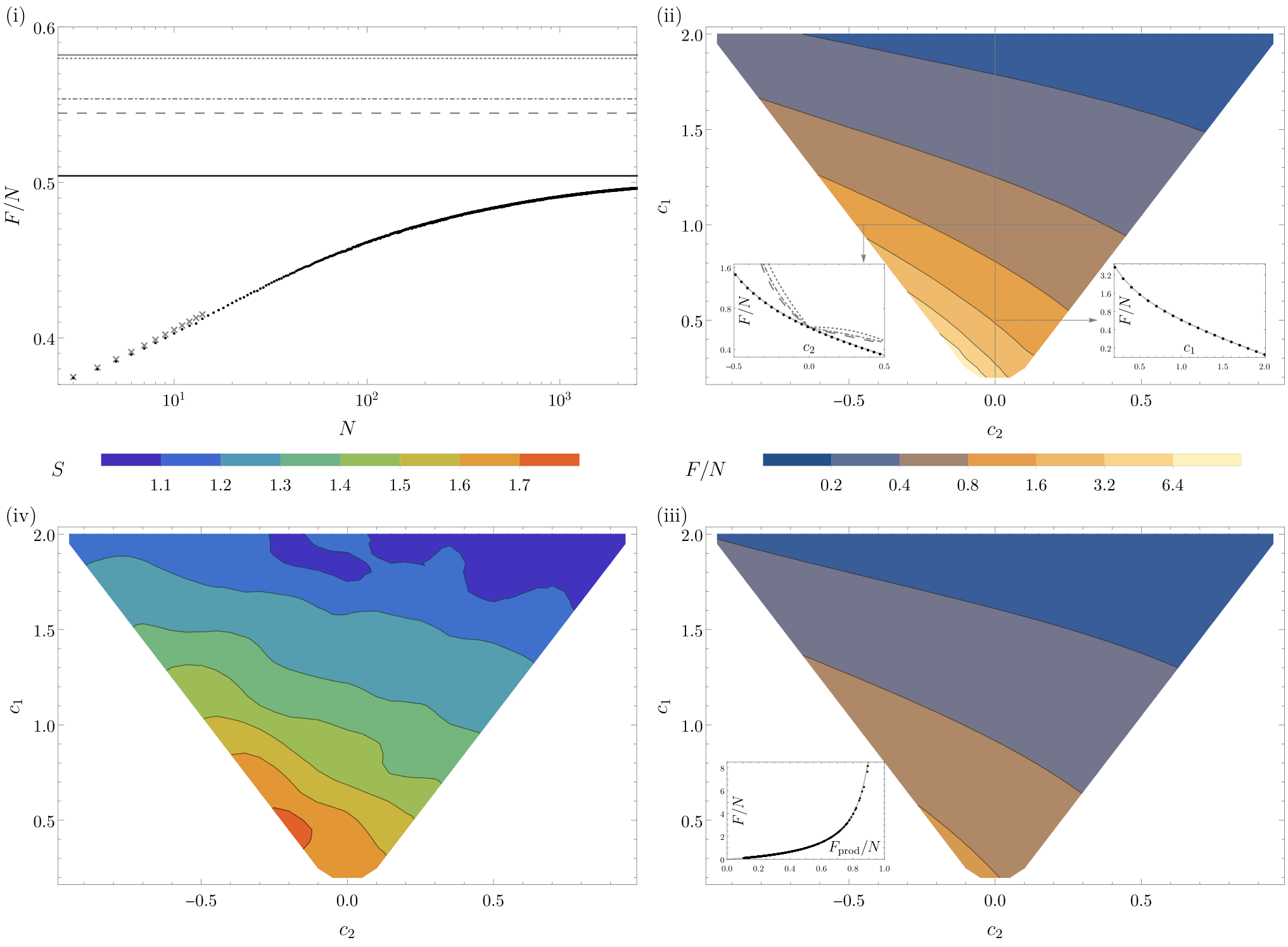
First, in Fig. 1(i) we present a comparison of results of the QFI optimization procedure for exemplary dephasing parameters , (correlated noise) obtained using the finite number of particles MPO approach and the asymptotic value of the QFI per particle obtained using the iMPO approach—note that we plot as we expect asymptotic linear scaling of the QFI and hence convergence of to a fixed value. The results obtained via the two approaches are in very good agreement. When we plot QFI versus and fit to the data for large a straight line we obtain a slope of . It compares well with the asymptotic limit obtained directly from the iMPO method as . This is a numerical confirmation that indeed the iMPO approach which, as described in Sec. III.4 is much more conceptually involved, yields correct results. This is a highly relevant observation as it is numerically much more efficient to obtain asymptotic properties of the QFI using directly the iMPO approach rather than performing finite computations and extrapolating them to . While performing the optimization we have set the error tolerance on the level of , which resulted in the maximal bond dimension required in the numerical procedure to be only for the input state and for the SLD. This demonstrates how efficient the MPO description is in this case. Crosses overlaid on the plot indicate the regime where direct calculations using the standard full Hilbert space description were possible on the same high performance PC on which the MPO algorithms were run. This regime is clearly very far from the one were we observe the convergence to the asymptotic linear scaling of the QFI with , and is only accessible numerically using the MPO based methods. In Fig. 1(ii) we present the contour plot depicting the asymptotic value of the QFI per particle as a function of noise parameters and contrast with the achievable QFI when using product states, see Fig. 1(iii). In order to appreciate the amount of entanglement that is present in the optimal states, in Fig. 1(iv) we provide a contour plot of the results of calculation of the von Neuman entropy for the iMPO Cirac et al. 2011 corresponding to the reduced density matrix of the system when half of the particles is traced out (optimal QFI can be achieved by many different states so some fluctuations of entropy are to be expected). We see a clear relation, between the amount of entanglement and the increase in sensing precision.
Let us now ask the question, whether some insight into the problem could have been gained by ingeniously adapting the state-of-the-art methods of deriving fundamental bounds in quantum metrology developed with uncorrelated noise models in mind Escher et al. 2011; Demkowicz-Dobrzański et al. 2012; Demkowicz-Dobrzański and Maccone 2014; Demkowicz-Dobrzański et al. 2017; Zhou et al. 2018. These methods provide easily calculable asymptotic bounds, based on just the knowledge of the Kraus operators of elementary probe dynamics or alternatively noise jump operators appearing in the quantum master equation. Even though the noise in our problem is correlated we can formally divide the evolution as a collection of independent channels acting on two, three or more particles—a similar trick has been employed in a recent study of the impact of many-body effects in atomic interferometry Czajkowski et al. 2018. In the scheme below we indicate the possible constructions. First we formally decompose local dephasing gates as products of local dephasing gates with corresponding and such that , and the unitary encoding gate as a product , where , are phase gates with corresponding phases , , such that . We can now unravel the total dynamics as effectively composed of independent channels , or group the gates into larger channels , or channel , etc.—see Fig. 2.
.
We may now apply the bounds derived for uncorrelated noise models Demkowicz-Dobrzański et al. 2012; Demkowicz-Dobrzański and Maccone 2014 using either decomposition of the dynamics into , or channels—we can group the operations in any way we please as in this case all elementary evolutions commute. In order to obtain the tightest bound we numerically optimize the split of phases as well as noise contributions between gates , and , , while making sure that the resulting is a legitimate quantum channel—note that the bare two qubit gate is not a proper quantum channel as it is not completely positive. The results obtained are depicted in the left inset of Fig. 1(ii). While the bounds are tight for the decorrelated noise model they are far from the actual achievable QFI in the correlated (or anti-correlated) noise regimes and as expected they improve when we increase the elementary channel size. Still, because this method scales badly with the elementary channel size we were forced to stop with channel. This demonstrates, that state-of-the-art methods developed with uncorrelated noise models in mind yield bounds that are far from satisfactory in case of correlated noise models.
As mentioned above, the use of the iMPO approach can greatly speed up process of calculating asymptotic value of QFI. In order to study the impact of noise correlations on the achievable QFI and the optimal states, for the rest of this section, we will therefore restrict ourselves to numerical results obtained using this approach. Using iMPO we have studied the optimal QFI for all noise parameters in the range , and . We were able to impose the 0.3% relative error on the obtained results, by going with state bond dimensions up to while keeping . In interesting to note, that in the studied here cases higher gave negligible gain in comparison to gain from increasing —this is most probably related with the fact that local uncorrelated measurement are close to optimal, a fact often encountered in quantum metrology studies when the QFI is the only figure of merit to be optimised.
The main qualitative feature that clearly emerges from the Fig. 1(ii) is the decrease of the optimal QFI with the increase of correlated noise part parameter . At the same time going into the anti-correlation regime (negative ) allows for a significant increase in the achievable QFI. This is to be expected as in the noise anti-correlation regime the noise operators responsible for correlations take the form of and are therefore linearly independent from the Hamiltonian operator which is a sum of . This is related with the fact that in the extreme case of perfect anti-correlations (no independent local dephasing noise component) it is possible to employ quantum error-correction inspired protocols in order to preserve the Heisenberg scaling Layden and Cappellaro 2018. This is also reflected by the divergent behaviour of the state-of-the-art based bounds, which take into account all possible adaptive estimation strategies—note that there is no analogous divergence in the numerical results we obtain as we consider a parallel sensing strategy involving the most general entangled input states and most general measurement but no adaptive strategies. This again indicates, that if one aims at determining the potential of parallel entangled based strategies in presence of noise correlations, the state-of-the-art methods provide bounds which are very far from the actually achievable performance. The line on the Fig. 1(ii) corresponds to the strictly local dephasing model for which exact asymptotically saturable bound is known and reads Escher et al. 2011; Demkowicz-Dobrzański et al. 2012, where . Our numerical results obtained using iMPO agree perfectly with this formula (see right inset on Fig. 1(ii)).
In case of purely local dephasing it is known that in the limit of large number of particles the fundamental bound, , can be saturated by protocols involving weakly spin squeezed states Ulam-Orgikh and Kitagawa 2001; Escher et al. 2011, e.g. one-axis twisted states Ma et al. 2011. Having obtained numerical optimal values of the QFI per particle using our MPO based methods, we want now to check whether the weakly spin squeezed strategy saturates the QFI in case of locally correlated noise model similarly as in the decorrelated noise scenario. For concreteness, consider the following one-axis squeezed state of particles:
| (63) |
where is the squeezing strength. We follow the standard protocol Ma et al. 2011, where the above state is rotated to the equator of the Bloch sphere so that the points in the direction, in a way that the direction in which the angular momentum has minimal variance is . The state is then subject to locally correlated dephasing evolution and is rotated by an unknown angle . Assuming we operate around , we measure the observable as this is the optimal choice in this case, from which value we infer the value of . Using the standard linear error propagation formula the resulting uncertainty of estimating the phase reads: . In order to calculate the above quantity we move to the Heisenberg picture. Since we operate around , we can replace , and plug everywhere. Under the locally correlated dephasing noise the relevant expectation values should be replaced according to the following rules:
| (64) | ||||
Taking the limit , in a way that we obtain that the relevant expectation values on the squeezed state read Ma et al. 2011 (assume ): , , , (). As a result while
| (65) |
This leads to the final formula for the asymptotic precision which can be related with the corresponding Fisher information per particle equal to:
| (66) |
We have checked that this formula agrees with our numerical results up to the desired accuracy (), and the representative comparison of the numerical data and this formula is provided in the left inset of Fig. 1(ii). This implies that similarly as in the uncorrelated dephasing models, weakly spin-squeezed states are asymptotically optimal. Note that this does not imply that the optimal MPO states we have obtained in our numerical procedure are these kind of states. Quite contrary, our MPO approach favours states with low bond dimension and local correlations, while the above states due to their fully symmetric nature correlate all the particles with each other irrespectively of their distance. Had we considered a product state strategy, the only modification in the above reasoning would be a substitution , which would lead to the corresponding QFI per particle:
| (67) |
which also agrees perfectly with the numerical results we have presented in Fig. 1(iii).
Using the above formula, we may also go back to the original problem of magnetic field sensing. Utilizing the relation we get the corresponding magnetic field sensing precision:
| (68) |
The above formula assumes a fixed interrogation time . We may generalize the considerations, and fix the total interrogation time which we allow to split into independent interrogation steps. The corresponding estimation uncertainty reads:
| (69) |
which when optimized over reaches the minimal value when and yields:
| (70) |
Based on the above results we can expect that weakly spin-squeezed states should also be optimal in case of a more general dephasing noise, provided the range of correlations is finite and we consider the asymptotic limit . In this case, following analogous calculations, we would arrive at the optimal magnetic field sensing precision of the form
| (71) |
where represent magnetic field correlations for particles at distance : . Comparing this result with the performance of the GHZ states for the same model, see Layden et al. 2019, we notice that there is the factor improvement in performance of the optimally spin-squeezed states over the GHZ states familiar from uncorrelated dephasing considerations Huelga et al. 1997; Ulam-Orgikh and Kitagawa 2001.
IV.2 Atomic clock stabilization
When one follows the Bayesian rather than the frequentist line of reasoning and focuses on minimization of the Bayesian variance, an apparently similar computational problem arises as in the cases of optimization of the QFI Macieszczak et al. 2014; Demkowicz-Dobrzański et al. 2015. The goal is then to minimize:
| (72) |
where and is a prior distribution for the parameter to be estimated (for simplicity we assume that the prior is centered at : ). The minimal achievable quadratic Bayesian cost for the problem, optimized over all measurements and estimators, reads Helstrom 1976; Macieszczak et al. 2014:
| (73) |
where is the variance of the prior distribution, is the output state averaged with the prior, while . It is clear from the above formula that the problem is computationally very similar to calculation of the QFI, as given in Eq. 8 (up to a replacement of the derivative of with )
An important problem where the Bayesian line of reasoning is relevant, and which at the same time is very well suited for our tensor network framework is the atomic clock stabilization problem. A typical atomic clock operates in a feedback loop where the local oscillator (LO, e.g. laser) is stabilised to atomic reference frequency by periodically interrogating atoms (using radiation from the LO) and based on the measured response, the frequency of the LO is corrected Ludlow et al. 2015. One of the main goals in the design of the clock interrogation scheme is to achieve the lowest instability typically quantified by the Allan variance (AVAR) Allan 1966; Riehle 2004:
| (74) |
where represents averaging over frequency fluctuations of the LO described by some stochastic process (which from the Bayesian estimation perspective plays the role of the prior distribution), denotes averaging time, atomic reference angular frequency and time-dependent angular frequency of the LO.
Fixing the physical properties of the atoms the goal is to optimize their initial states states, interrogations times, measurements and feedback corrections in order to minimize the AVAR. Performing such a comprehensive optimization is not feasible. In Chabuda et al. 2016 a lower bound on the achievable AVAR was introduced the quantum Allan Variance (QAVAR):
| (75) | ||||
| (76) |
where is the AVAR of free running LO, represents a correction to it from the feedback loop and is the interrogation time. We do not provide here explicit forms of the operators and and refer the interested reader to Chabuda et al. 2016, but just note that they are analogs of , as defined in the simple Bayesian estimation problem in Eq. (73). The important information is that, if the atoms with which the atomic clock interacts are described via states on some dimensional Hilbert space , then the and objects act on a tensor space , where is the number of atomic cycles that need to be considered in order to calculate QAVAR. We assume here an idealized situation that one cycle of atomic clock operation lasts —there is no dead time, and all the time is dedicated to interrogation of atoms by the LO. Typically we will think of the dimensional spaces of atomic states as being a fully symmetric subspace of two-level systems representing the relevant clock transition levels of the atoms—therefore we will use the notation for the states , which correspond to the symmetric state, where atoms are in an excited state and atoms in the ground state. Interaction between the LO and the atomic sample has form of Ramsey interferometry and after a single interrogation step will effectively encode the phase in the above written state as , where is the detuning of the LO frequency from the atomic reference frequency . The effect of LO fluctuations is equivalent to collective dephasing of atoms and hence the state will remain within the symmetric subspace—note that we are talking about the single Hilbert space here which will be represented by single node in the MPO framework. The key feature from our perspective is the fact that the LO frequency fluctuations are temporally correlated, and hence the collective dephasing acting on atoms at different interrogation steps (in our representation different steps are formally represented as different product subsystems in the space) will be correlated.
Assuming that LO fluctuations have finite correlations in time we can expect that QAVAR can be efficiently calculated using a tensor network in the form of a chain of length with -dimensional physical indices on each site. Apart from a clear numerical efficiency advantages, the use of tensor networks approach also allows us to constrain the class of input states to be product (bond dimension ) which corresponds to the typical situation in which atomic samples in different time steps are independent of each other, as they prepared anew at the beginning of each interrogation step—note that we will still consider entanglement between physical atoms with which the LO interacts at a given interrogation time step.
LO fluctuations can be characterized by the autocorrelation function which for the purpose of our example we choose to be a combination of Ornstein–Uhlenbeck (OU) process and white Gaussian frequency noise:
| (77) |
where we can interpret parameters , as strength of respectively OU process and white noise and as OU correlation range. We choose , , for which noise correlations on the time scale that will correspond to the optimal interrogation time step (which in this case will happen to be around ) will be weak enough so that they will appreciable affect only the nearest-neighbour “time-step subsystems”—studying noise with further correlations is possible but would require more computational resources because of the larger bond dimensions. For such a noise the AVAR of the free running LO reads:
| (78) |
and in the most interesting regime of large averaging times takes the form . We expect that in this limit QAVAR also takes the form with some constant which we will refer to as asymptotic coefficient.
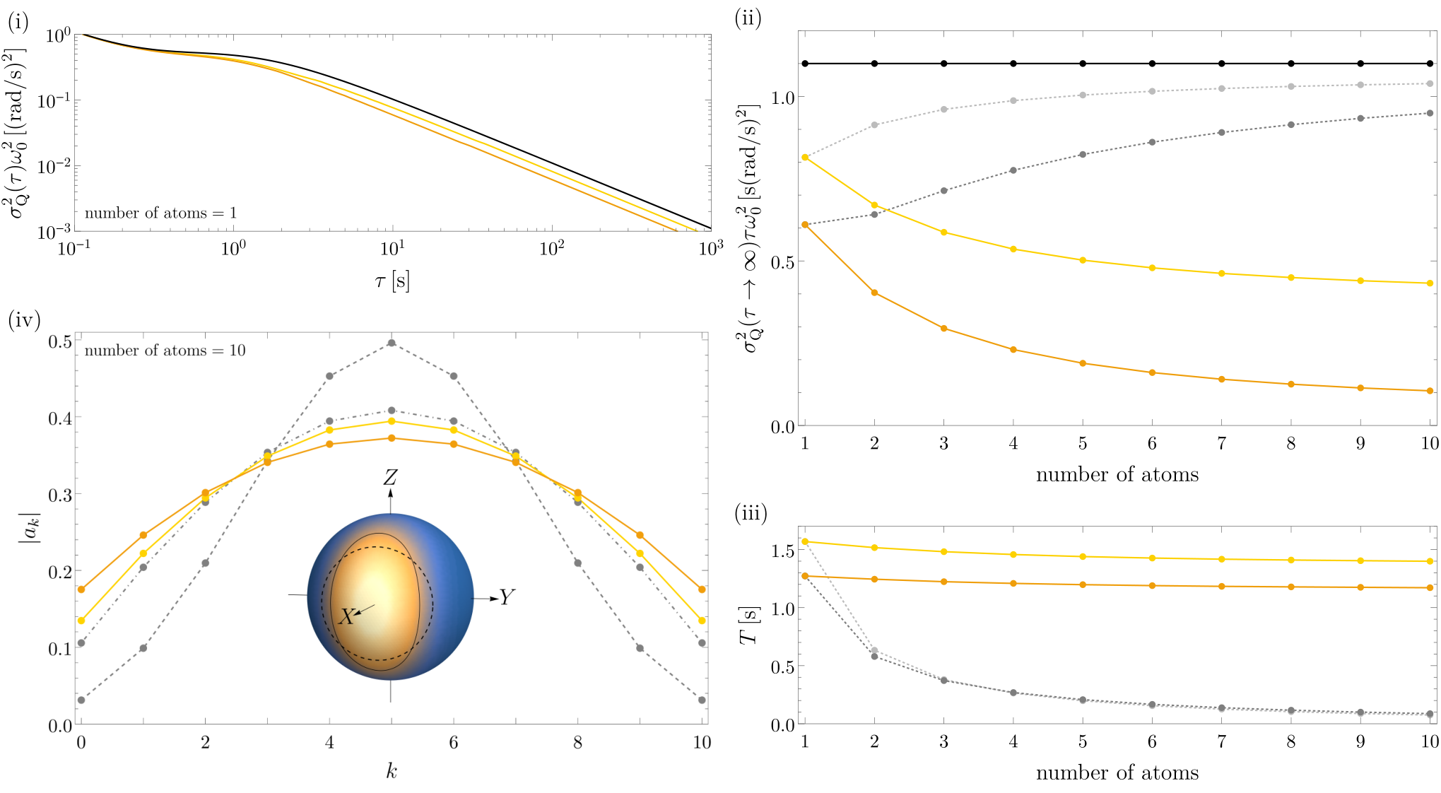
These calculations have been attempted in Chabuda et al. 2016 using the full Hilbert space description, but were not capable of approaching the regime where the character of the scaling of the QAVAR and the coefficient could be unambiguously read out. The tensor network framework, proposed in this paper, allows us to calculate QAVAR in previously inaccessible regime of large . In Fig. 3(i) we present the exemplary results for an atomic clock operating on one two-level atom which also shows that completely neglecting noise correlations in analysing the clock performance is unjustified. We see that the QAVAR curve flatten for , which when taking into account the optimal interrogation times which in this case approaches , implies that for calculations of the QAVAR we would need to consider interrogation steps and hence if full Hilbert space description was used for this purpose would require dimensional space—clearly an impossible task. Similarly as in the previous example, we may directly access the asymptotic behaviour () of the QAVAR function with the help of the iMPO approach. Following this approach we calculate the QAVAR asymptotic coefficient and the corresponding optimal interrogation time as a function of the number of atoms in the clock, see Fig. 3(ii-iii). From this figures we see that the differences in QAVAR between cases with strictly local noise and when nearest neighbour noise correlations are included only grow with the increasing number of atoms. This implies that noise correlations play an important role in the accurate analysis of clock performance. Note that, the definition (74) of the AVAR leads to an intrinsically not translationally invariant MPO for in the expression for QAVAR. Because of this when implementing the iMPO approach we approximate AVAR by an asymptotically equivalent expression:
| (79) |
which coincide with previous definition for much larger then the noise correlation length (which is exactly the regime in which iMPO approach operates). In order to keep relative errors below the numerical calculations required bond dimension for finite case and in the case of the iMPO approach.
We confront the results (which are optimized over the input state) with values obtained using a NOON/GHZ states as an input, . The NOON states are highly prone to dephasing noise, and hence the optimal interrogation times will be necessary reduced compared to the optimal (more robust states). This is visible in the Fig. 3(ii-iii), where we see that even though the optimal for the NOON state scales down (in fact as ), the noise quickly destroys any gain from the feedback loop to AVAR of a free running LO. This is a manifestation of a generic poor performance of the NOON/GHZ states in realistic (noisy) scenarios with increasing particle number Huelga et al. 1997; Escher et al. 2011; Demkowicz-Dobrzański et al. 2012.
Our framework allow us also to easily study the optimal input states. In Fig. 3(iv) we plot the absolute values of the probability amplitudes for the optimal states (for LO noise which is strictly local or also includes the nearest neighbours correlations) alongside for coherent spin state (CSS) and the sine state Berry and Wiseman 2000 (which is the optimal input state for Bayesian estimation of phase with a flat prior distribution). We see that our optimal states are nonclassical, which we can quantify by calculating their spin-squeezing parameter Ma et al. 2011 which is for CSS, for sine state, and for the optimal states for LO noise which is respectively strictly local or also includes the nearest neighbours correlations (squeezing in this last case can be also observed from Husimi Q distribution on Bloch sphere in the centre of the Fig. 3(iv)).
IV.3 Fidelity susceptibility calculations for many-body thermal states
In condensed matter context, fidelity between many-body states and , that differ by a small variation of a parameter in a Hamiltonian, is a mean to identify the location of a phase transition Zanardi and Paunković 2006; Rams and Damski 2011. This is where the fidelity susceptibility , defined by , has a maximum indicating a fundamental change in the state of the system. This concept was employed in Ref. Rams et al. 2018 to evaluate the usefulness of a quantum phase transition, that happens at zero temperature, for precise sensing of the parameter in a realistic system at a finite temperature. QFI defines a metric in the space of quantum states (the Bures metric)Braunstein and Caves 1994 and is directly related with the fidelity susceptibility, namely .
Unlike at zero temperature, the fidelity between a thermal many-body states represented by MPOs is not tractable in general. This is why a quasi-fidelity was employed defining a quasi-susceptibility, , that provides bounds for the exact fidelity susceptibility Albuquerque et al. 2010; Sirker 2010:
| (80) |
The Hamiltonian considered in Ref. Rams et al. 2018 was the spin- XX model
| (81) |
with a quantum critical point at . Taking the MPOs studied in Ref. Rams et al. 2018, we bypass the tractability problem employing the part of our scheme with to calculate the QFI . This exact susceptibility for the chain with spins is shown in Fig. 4 together with the upper and lower bounds (80). The accuracy of the fidelity susceptibility is limited by the finite bond dimension as well the finite parameter difference . Nevertheless, we obtain satisfying results with relative error around for and .
This example demonstrates that the scheme for calculating fidelity susceptibility is a useful byproduct of our general algorithm. Beyond the present metrological context, it paves a way to generalize the zero-temperature fidelity approach to detecting quantum phase transitions Zanardi and Paunković 2006; Rams and Damski 2011—by now standard in condensed matter physics—to phase transitions in quantum many-body systems at finite temperature. Their thermal states can be represented either by MPO, when DMRG on a cylinder is employed Chen et al. 2018, or its two-dimensional generalization on an infinite lattice (iPEPO) Czarnik et al. 2016; Czarnik and Corboz 2019.
V Conclusions
We have provided a comprehensive framework for optimization of quantum metrological protocols using the MPO/MPS formalism. The potential to deal effectively with correlated noise models as well as directly access the asymptotic is what makes this framework unique. We also expect that this framework may also be adapted to deal with even more challenging metrological problems including noisy multiparameter estimation Ragy et al. 2016; Szczykulska et al. 2016; Baumgratz and Datta 2016, waveform estimation Tsang et al. 2011; Berry et al. 2013 or the study of the effectiveness of adaptive metrological protocols including quantum error correction based schemes Arrad et al. 2014; Dür et al. 2014; Zhou et al. 2018; Layden and Cappellaro 2018; Gorecki et al. 2019. We also expect that this numerical framework may be crucial for understanding better metrological models with temporally correlated noise especially of non-Markovian nature Chin et al. 2012, where effective tools to find the optimal metrological protocols in such cases are yet to be developed.
Acknowledgements.
We would like to thank Marek M. Rams, David Layden, Maciej Lewenstein, Shi-Ju Ran, Piet O. Schmidt and Ian D. Leroux for fruitful discussions. We are also indebt to Marek M. Rams for sharing with us the data from Ref. Rams et al. 2018. KCh and RDD acknowledge support from the National Science Center (Poland) grant No. 2016/22/E/ST2/00559. Work of JD was funded by NCN together with European Union through QuantERA ERA NET program 2017/25/Z/ST2/03028. TJO was supported, in part, by the DFG through SFB 1227 (DQmat), the RTG 1991, and the cluster of excellence EXC 2123 QuantumFrontiers.References
- Giovannetti et al. (2006) V. Giovannetti, S. Lloyd, and L. Maccone, Phys. Rev. Lett. 96, 010401 (2006).
- Paris (2009) M. G. A. Paris, Int. J. Quantum Inf. 07, 125 (2009).
- Tóth and Apellaniz (2014) G. Tóth and I. Apellaniz, Journal of Physics A: Mathematical and Theoretical 47, 424006 (2014).
- Demkowicz-Dobrzański et al. (2015) R. Demkowicz-Dobrzański, M. Jarzyna, and J. Kołodyński, in Progress in Optics, Vol. 60, edited by E. Wolf (Elsevier, 2015) pp. 345 – 435.
- Schnabel (2017) R. Schnabel, Physics Reports 684, 1 (2017).
- Degen et al. (2017) C. L. Degen, F. Reinhard, and P. Cappellaro, Rev. Mod. Phys. 89, 035002 (2017).
- Pezzè et al. (2018) L. Pezzè, A. Smerzi, M. K. Oberthaler, R. Schmied, and P. Treutlein, Rev. Mod. Phys. 90, 035005 (2018).
- Pirandola et al. (2018) S. Pirandola, B. R. Bardhan, T. Gehring, C. Weedbrook, and S. Lloyd, Nat. Photonics 12, 724 (2018).
- Feynman (1982) R. P. Feynman, International Journal of Theoretical Physics 21, 467 (1982).
- Aolita et al. (2015) L. Aolita, C. Gogolin, M. Kliesch, and J. Eisert, Nature Communications 6, 8498 EP (2015).
- Cramer et al. (2010) M. Cramer, M. B. Plenio, S. T. Flammia, R. Somma, D. Gross, S. D. Bartlett, O. Landon-Cardinal, D. Poulin, and Y.-K. Liu, Nature Communications 1, 149 EP (2010).
- Dorner (2012) U. Dorner, New Journal of Physics 14, 043011 (2012).
- Macieszczak et al. (2014) K. Macieszczak, M. Fraas, and R. Demkowicz-Dobrzański, New Journal of Physics 16, 113002 (2014).
- Escher et al. (2011) B. M. Escher, R. L. de Matos Filho, and L. Davidovich, Nature Phys. 7, 406 (2011).
- Demkowicz-Dobrzański et al. (2012) R. Demkowicz-Dobrzański, J. Kołodyński, and M. Guţă, Nat. Commun. 3, 1063 (2012).
- Kołodyński and Demkowicz-Dobrzański (2013) J. Kołodyński and R. Demkowicz-Dobrzański, New Journal of Physics 15, 073043 (2013).
- Knysh et al. (2014) S. I. Knysh, E. H. Chen, and G. A. Durkin, (2014), arXiv:1402.0495 [quant-ph] .
- Demkowicz-Dobrzański and Maccone (2014) R. Demkowicz-Dobrzański and L. Maccone, Phys. Rev. Lett. 113, 250801 (2014).
- Sekatski et al. (2017) P. Sekatski, M. Skotiniotis, J. Kołodyński, and W. Dür, Quantum 1, 27 (2017).
- Demkowicz-Dobrzański et al. (2017) R. Demkowicz-Dobrzański, J. Czajkowski, and P. Sekatski, Phys. Rev. X 7, 041009 (2017).
- Zhou et al. (2018) S. Zhou, M. Zhang, J. Preskill, and L. Jiang, Nat. Commun. 9, 78 (2018).
- Ludlow et al. (2015) A. D. Ludlow, M. M. Boyd, J. Ye, E. Peik, and P. O. Schmidt, Rev. Mod. Phys. 87, 637 (2015).
- André et al. (2004) A. André, A. S. Sørensen, and M. D. Lukin, Phys. Rev. Lett. 92, 230801 (2004).
- Borregaard and Sørensen (2013) J. Borregaard and A. S. Sørensen, Phys. Rev. Lett. 111, 090801 (2013).
- Kessler et al. (2014) E. M. Kessler, P. Kómár, M. Bishof, L. Jiang, A. S. Sørensen, J. Ye, and M. D. Lukin, Phys. Rev. Lett. 112, 190403 (2014).
- Chabuda et al. (2016) K. Chabuda, I. D. Leroux, and R. Demkowicz-Dobrzański, New Journal of Physics 18, 083035 (2016).
- Clerk et al. (2010) A. A. Clerk, M. H. Devoret, S. M. Girvin, F. Marquardt, and R. J. Schoelkopf, Rev. Mod. Phys. 82, 1155 (2010).
- Szańkowski et al. (2017) P. Szańkowski, G. Ramon, J. Krzywda, D. Kwiatkowski, and Ł. Cywiński, Journal of Physics: Condensed Matter 29, 333001 (2017).
- Chin et al. (2012) A. W. Chin, S. F. Huelga, and M. B. Plenio, Phys. Rev. Lett. 109, 233601 (2012).
- Rondin et al. (2014) L. Rondin, J.-P. Tetienne, T. Hingant, J.-F. Roch, P. Maletinsky, and V. Jacques, Reports on Progress in Physics 77, 056503 (2014).
- Paz-Silva et al. (2017) G. A. Paz-Silva, L. M. Norris, and L. Viola, Phys. Rev. A 95, 022121 (2017).
- Kwiatkowski and Cywiński (2018) D. Kwiatkowski and L. Cywiński, Phys. Rev. B 98, 155202 (2018).
- Jeske et al. (2014) J. Jeske, J. H. Cole, and S. F. Huelga, New Journal of Physics 16, 073039 (2014).
- Altenburg et al. (2017) S. Altenburg, M. Oszmaniec, S. Wölk, and O. Gühne, Phys. Rev. A 96, 042319 (2017).
- Apellaniz et al. (2018) I. Apellaniz, I. Urizar-Lanz, Z. Zimborás, P. Hyllus, and G. Tóth, Phys. Rev. A 97, 053603 (2018).
- Jarzyna and Demkowicz-Dobrzański (2013) M. Jarzyna and R. Demkowicz-Dobrzański, Phys. Rev. Lett. 110, 240405 (2013).
- Bridgeman and Chubb (2017) J. C. Bridgeman and C. T. Chubb, Journal of Physics A: Mathematical and Theoretical 50, 223001 (2017).
- Fannes et al. (1992) M. Fannes, B. Nachtergaele, and R. F. Werner, Comm. Math. Phys. 144, 443 (1992).
- Östlund and Rommer (1995) S. Östlund and S. Rommer, Phys. Rev. Lett. 75, 3537 (1995).
- Verstraete and Cirac (2004) F. Verstraete and J. I. Cirac, (2004), arXiv:cond-mat/0407066 [cond-mat.str-el] .
- Vidal (2007) G. Vidal, Phys. Rev. Lett. 99, 220405 (2007).
- Zwolak and Vidal (2004) M. Zwolak and G. Vidal, Phys. Rev. Lett. 93, 207205 (2004).
- Verstraete et al. (2004a) F. Verstraete, J. J. García-Ripoll, and J. I. Cirac, Phys. Rev. Lett. 93, 207204 (2004a).
- Cincio and Vidal (2013) L. Cincio and G. Vidal, Phys. Rev. Lett. 110, 067208 (2013).
- Nielsen and Chuang (2000) M. A. Nielsen and I. L. Chuang, Quantum Computing and Quantum Information (Cambridge University Press, 2000).
- Helstrom (1976) C. W. Helstrom, Quantum detection and estimation theory (Academic Press, 1976).
- Holevo (1982) A. S. Holevo, Probabilistic and Statistical Aspects of Quantum Theory (North Holland, 1982).
- Braunstein and Caves (1994) S. L. Braunstein and C. M. Caves, Phys. Rev. Lett. 72, 3439 (1994).
- Macieszczak (2013) K. Macieszczak, (2013), arXiv:1312.1356 [quant-ph] .
- Demkowicz-Dobrzański (2011) R. Demkowicz-Dobrzański, Phys. Rev. A 83, 061802(R) (2011).
- Tóth and Vértesi (2018) G. Tóth and T. Vértesi, Phys. Rev. Lett. 120, 020506 (2018).
- Breuer and Petruccione (2002) H.-P. Breuer and F. Petruccione, The Theory of Open Quantum Systems (Oxford University Press, 2002).
- Trotter (1959) H. F. Trotter, Proc. Amer. Math. Soc. 10, 545 (1959).
- Suzuki (1966) M. Suzuki, Journal of the Physical Society of Japan 21, 2274 (1966).
- Suzuki (1976) M. Suzuki, Progress of Theoretical Physics 56, 1454 (1976).
- Dorner et al. (2009) U. Dorner, R. Demkowicz-Dobrzanski, B. J. Smith, J. S. Lundeen, W. Wasilewski, K. Banaszek, and I. A. Walmsley, Phys. Rev. Lett. 102, 040403 (2009).
- Hastings (2007) M. B. Hastings, Journal of Statistical Mechanics: Theory and Experiment 2007, P08024 (2007).
- Verstraete et al. (2004b) F. Verstraete, D. Porras, and J. I. Cirac, Phys. Rev. Lett. 93, 227205 (2004b).
- Vidal (2003) G. Vidal, Phys. Rev. Lett. 91, 147902 (2003).
- Vidal (2004) G. Vidal, Phys. Rev. Lett. 93, 040502 (2004).
- White (1992) S. R. White, Phys. Rev. Lett. 69, 2863 (1992).
- Schollwöck (2011) U. Schollwöck, Annals of Physics 326, 96 (2011).
- Corboz (2016) P. Corboz, Phys. Rev. B 94, 035133 (2016).
- Huelga et al. (1997) S. F. Huelga, C. Macchiavello, T. Pellizzari, A. K. Ekert, M. B. Plenio, and J. I. Cirac, Phys. Rev. Lett. 79, 3865 (1997).
- van Kampen (1981) N. G. van Kampen, Stochastic Processes in Physics and Chemistry (Elsevier, 1981).
- Pfeifer et al. (2014) R. N. C. Pfeifer, G. Evenbly, S. Singh, and G. Vidal, (2014), arXiv:1402.0939 [physics.comp-ph] .
- Cirac et al. (2011) J. I. Cirac, D. Poilblanc, N. Schuch, and F. Verstraete, Phys. Rev. B 83, 245134 (2011).
- Czajkowski et al. (2018) J. Czajkowski, K. Pawłowski, and R. Demkowicz-Dobrzański, New Journal of Physics 21, 053031 (2019).
- Layden and Cappellaro (2018) D. Layden and P. Cappellaro, npj Quantum Inf. 4, 30 (2018).
- Ulam-Orgikh and Kitagawa (2001) D. Ulam-Orgikh and M. Kitagawa, Phys. Rev. A 64, 052106 (2001).
- Ma et al. (2011) J. Ma, X. Wang, C. Sun, and F. Nori, Physics Reports 509, 89 (2011).
- Layden et al. (2019) D. Layden, S. Zhou, P. Cappellaro, and L. Jiang, Phys. Rev. Lett. 122, 040502 (2019).
- Allan (1966) D. W. Allan, Proceedings of the IEEE 54, 221 (1966).
- Riehle (2004) F. Riehle, Frequency Standards Basics and Applications (WILEY-VCH, 2004).
- Berry and Wiseman (2000) D. W. Berry and H. M. Wiseman, Phys. Rev. Lett. 85, 5098 (2000).
- Albuquerque et al. (2010) A. F. Albuquerque, F. Alet, C. Sire, and S. Capponi, Phys. Rev. B 81, 064418 (2010).
- Sirker (2010) J. Sirker, Phys. Rev. Lett. 105, 117203 (2010).
- Zanardi and Paunković (2006) P. Zanardi and N. Paunković, Phys. Rev. E 74, 031123 (2006).
- Rams and Damski (2011) M. M. Rams and B. Damski, Phys. Rev. Lett. 106, 055701 (2011).
- Rams et al. (2018) M. M. Rams, P. Sierant, O. Dutta, P. Horodecki, and J. Zakrzewski, Phys. Rev. X 8, 021022 (2018).
- Chen et al. (2018) B.-B. Chen, L. Chen, Z. Chen, W. Li, and A. Weichselbaum, Phys. Rev. X 8, 031082 (2018).
- Czarnik et al. (2016) P. Czarnik, M. M. Rams, and J. Dziarmaga, Phys. Rev. B 94, 235142 (2016).
- Czarnik and Corboz (2019) P. Czarnik and P. Corboz, Phys. Rev. B 99, 245107 (2019).
- Ragy et al. (2016) S. Ragy, M. Jarzyna, and R. Demkowicz-Dobrzański, Phys. Rev. A 94, 052108 (2016).
- Szczykulska et al. (2016) M. Szczykulska, T. Baumgratz, and A. Datta, Advances in Physics: X 1, 621 (2016).
- Baumgratz and Datta (2016) T. Baumgratz and A. Datta, Phys. Rev. Lett. 116, 030801 (2016).
- Tsang et al. (2011) M. Tsang, H. M. Wiseman, and C. M. Caves, Phys. Rev. Lett. 106, 090401 (2011).
- Berry et al. (2013) D. W. Berry, M. J. W. Hall, and H. M. Wiseman, Phys. Rev. Lett. 111, 113601 (2013).
- Arrad et al. (2014) G. Arrad, Y. Vinkler, D. Aharonov, and A. Retzker, Phys. Rev. Lett. 112, 150801 (2014).
- Dür et al. (2014) W. Dür, M. Skotiniotis, F. Fröwis, and B. Kraus, Phys. Rev. Lett. 112, 080801 (2014).
- Gorecki et al. (2019) W. Gorecki, S. Zhou, L. Jiang, and R. Demkowicz-Dobrzanski, (2019), arXiv:1901.00896 [quant-ph] .