Gravitational wave observations, distance measurement uncertainties, and cosmology

We assume that the BNS inspirals in quasi-circular orbits, and neglect the effects of both spin and tidal deformability. Furthermore, we assume that the sky position, identified by the right ascension $\alpha$ and declination $\delta$, as well as the redshift $z$ of the source are known thanks to the observation of an electromagnetic counterpart. The GW waveform emitted by the inspiralling BNS in the wave propagation frame Maggiore 2008, is then given by

with

and where $\phi_{c}$ is the phase at the coalescence time $t_{c}$. We consider amplitude and phase evolutions described by the lowest order approximation in the Post-Newtonian expansion given, e.g., in Sathyaprakash and Schutz 2009. At this approximation order, the amplitude and phase only depends upon the chirp mass $\mathcal{M}={(m_{1}m_{2})^{3/5}}{(m_{1}+m_{2})^{-1/5}}$.

We define the parameter $v\equiv\cos(\iota)$ with $\iota$ the inclination of the orbital plane, i.e., the angle between the angular momentum of the binary and the line-of-sight, so that for face-on binaries $v=\pm 1$, while for edge-on binaries $v=0$ . The two GW polarizations are indicated by a capital latin index, $A,B=(+,\times)$, and in the following we use the Einstein summation convention.

By Fourier transforming Eqs. (1), and using the stationary phase approximation Finn and Chernoff 1993 one finds

where we have factored out explicitly the $v$, $D$ and $\phi_{c}$ dependence, and where

and

In the detector reference frame — denoted by a lowercase latin index — the signal is characterized by the dimensionless strain $\tilde{h}_{a}$. We denote by $n_{d}$ is the total number of detectors, so $a=1,\ldots n_{d}$. The fractional change of length in an interferometer is obtained by projecting onto the detector arms with the two “antenna patterns” $F^{+}_{a}$ and $F^{\times}_{a}$ for the two polarizations Jaranowski et al. 1998. These depend on the sky position of the GW source (right ascension $\alpha$ and declination $\delta$), on the polarization angle $\psi$, and on time $t$. For CBC signals, $F^{A}_{a}$ are essentially constant during the entire duration of the signal, so that we can drop the $t$ dependence. The terms in $\psi$ in the antenna response functions can be factorized using a rotation matrix Cutler and Flanagan 1994

such that,

where $\hat{F}^{A}_{a}\equiv F^{A}_{a}(\alpha,\delta,\psi=0)$. In the frequency domain, the signal in the detector reference frame can by obtained from Eqs. (4) and (7) as

where we have added a delay term $\tau_{a}$ relative to the time travel of the GW from the center of the geocentric frame to the detector.

From Eq. (8), the signal phase depends on the two intrinsic parameters¹¹ 1 At higher PN order, the spins should be also taken into account Sathyaprakash and Schutz 2009. $\mathcal{M}$ and $t_{c}$. There are also extrinsic parameters, namely the source sky coordinates $\alpha,\delta$ (that are assumed to be known) and four other parameters $D,\phi_{c},v$ and $\psi$ which determine the amplitude scale of the GW signal. These latter parameters are recovered from the measurement of the GW polarization amplitudes $+$ and $\times$. In principle, a noise-free signal observed in at least three detectors leads to a perfect measurement of the two polarizations $+$ and $\times$, and thus enables us to completely solve for these four variables. However, this is not true in practise, as the presence of noise and correlations between those parameters greatly limits the accuracy of their estimates, and the detector network may not be sensitive to both polarizations.

In order to understand the main sources of error on the distance $D$, we briefly summarize the canonical data analysis-framework for matched filtering. In the following, the output (data, noise, etc) associated with the $n_{d}$-detector network will be denoted by $\vec{x}=(x_{1},\ldots,x_{n_{d}})$.

The data $\vec{s}$ is modelled as a superposition of noise $\vec{\eta}$ and signal $\vec{h}(\boldsymbol{\theta})$, where $\boldsymbol{\theta}$ are the set of eight parameters introduced previously,

We assume that the noise $\vec{\eta}$ is stationary, Gaussian distributed with zero mean and it is uncorrelated between different detectors²² 2 We consider detectors separated by large distances, $\gtrsim$ 1000 km so that the noise in the observable frequency bandwidth can be reasonably assumed uncorrelated.. The likelihood for a signal $\vec{h}$ to be present in the detector data $\vec{s}$ is Jaranowski and Królak 2012

where the scalar product is defined by

where a sum over the detectors $a$ is understood. Here, ‘*’ denotes complex conjugation, and $S_{n,a}(f)$ is the one-sided power spectral density of the detector $a$. The posterior distribution for having a signal $\vec{h}$ is given by

where $\pi$ represents the prior belief for the signal parameters. The uncertainties on the recovery of the parameters $\boldsymbol{\theta}$ is encoded in the posterior distributions. We can hence estimate the uncertainties on the distance evaluation by marginalizing over all the GW parameters with the exception of the distance.

We focus on the extrinsic parameters $\boldsymbol{\beta}=(D,\phi_{c},v,\psi)$, assuming a given sky position and intrinsic parameters for the GW event. Following Cutler and Flanagan 1994 we define the amplitude factors

so that from Eq. (8),

where $\vec{n}$ denotes the vector pointing to the source and is a short-hand notation for the source sky position $(\alpha,\delta)$. The scalar product $\braket{\vec{h}|\vec{h^{\prime}}}$ in Eq. (11) between the GW signal $h$ and the template $h^{\prime}$ then becomes

We use the prime to denote template related extrinsic parameters $\boldsymbol{\beta^{\prime}}$ (template and signal have the same intrinsic parameters). From Eqs. (11) and (13), the matrix $\Theta^{AB}$ reads

where, for uncorrelated detectors, the $n_{d}\times n_{d}$ matrix $\kappa^{ab}$ is given by

Here $S_{n,aver}$ is the average, over all the detectors, of the spectral noise densities, viz.

so that the matrix $\kappa^{ab}$ is real and diagonal, with weights given by the noise power spectral density for each detector. Finally $\braket{\tilde{k}|\tilde{k}}$ is given by

The matrix $\Theta^{AB}$ is a real non-diagonal symmetric matrix which incorporates information on position of the source in the sky, as well as geometrical information of the detector network, weighted by the detectors sensitivity $\kappa^{ab}$. This matrix is independent of the polarization angle $\psi$, and characterizes the response of the detector network to the $+$ and $\times$ polarizations with $\psi=0$.

The matrix $\Theta^{AB}$ can be diagonalized by

with

This is equivalent to defining effective polarizations $\bar{+}$ and $\bar{\times}$ obtained from the original $+$ and $\times$ by rotating the definition of $\psi$ by the angle $\Delta\psi$. The detector response $\bar{\Theta}^{AB}$ to $\bar{+}$ and $\bar{\times}$ takes the simple form

where $\sigma_{d}\equiv(\Theta^{++}+\Theta^{\times\times})/2$ and $0\leq\epsilon_{d}\leq 1$. Both those quantities can be also expressed in terms of the antenna patterns $\hat{F}^{A}_{a}(\vec{n})$.

The parameter $\epsilon_{d}$ indicates how well the effective polarization amplitudes can be measured from the detector network data Cutler and Flanagan 1994. When $\epsilon_{d}=0$, $\bar{+}$ and $\bar{\times}$ can be estimated equally well. For $\epsilon_{d}=1$, only $\bar{+}$ can be estimated. We elaborate further on this point in Sec. IV.1.

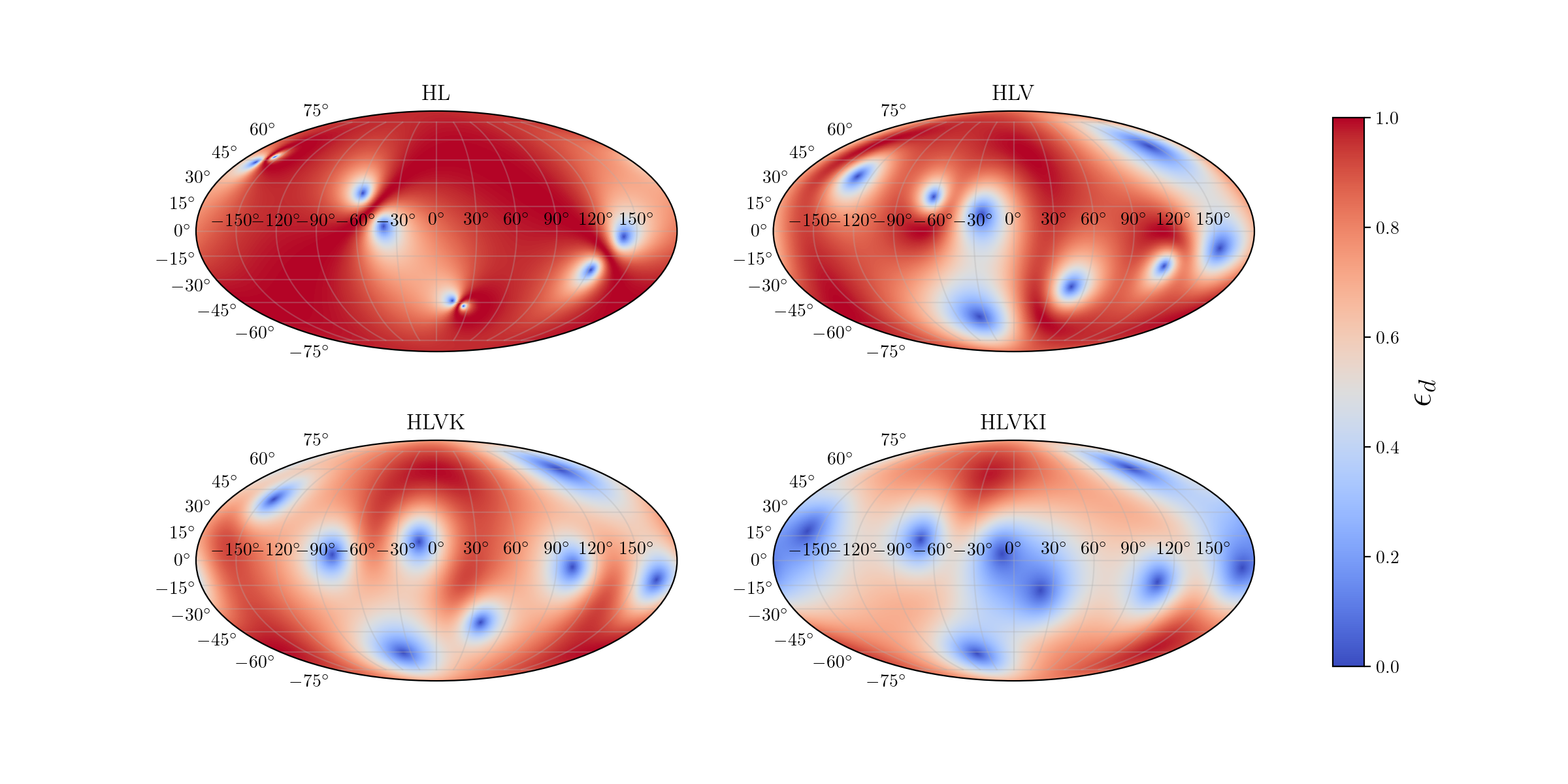
Fig. 1 shows the sky distribution of the parameter $\epsilon_{d}$ for different networks of GW detectors (we also show, for comparison, a similar plot for $\sigma_{d}$ in Fig. 2). Clearly, the areas where both polarizations can be better disentangled ($\epsilon_{d}$ small) expand when the number of detectors increases.

Assuming GW sources are equally distributed in the sky, Fig. 3 shows the probability that the source position has an $\epsilon_{d}$ value lower than a certain threshold. About 80 % of the sources have $\epsilon_{d}\lesssim 0.8$ for the five detector network HLVKI³³ 3 The labels “H”, “L”, “V”, “K”, “I” refers to the detectors present in the network, and corresponds to LIGO Hanford, LIGO Livingston, Virgo, Kagra and LIGO India, respectively. whereas this is less than 10 % of the sources for the two detector network HL. Using the effective polarization amplitudes $\bar{\mathcal{A}}_{B}={\cal A}_{B}(\bar{\psi}=\psi+\Delta\psi)$, Eq. (15) takes the form

On substituting Eq. (22) into Eq. (23), we find

with

where $\chi_{+}$ is given in (5), and

Finally, using (24), the network SNR is given by

where, on using (6a),

For a source that is overhead, $\sigma_{d}=n_{d}/2$. If the source is also face-on (i.e., $\chi_{+}=1$), it follows from Eq. (27) that $\rho^{2}=n_{d}\rho_{0}^{2}$. Thus $\rho_{0}$ can be interpreted as the single-detector SNR for a face-on source located overhead Cutler and Flanagan 1994.

The posterior probability density $P({\boldsymbol{\beta^{\prime}}}|\vec{s})$ for the extrinsic parameters ${\boldsymbol{\beta^{\prime}}}=(D^{\prime},\bar{\psi^{\prime}},v^{\prime},\phi^{\prime}_{c})$ given detector data $\vec{s}$, can be computed from the above identities. The source sky location and intrinsic parameters $\boldsymbol{\lambda^{\prime}}=(\alpha^{\prime},\delta^{\prime},\mathcal{M^{\prime}},t^{\prime}_{c})$ are known and can be factored out, so that from Eq. (12) we have⁴⁴ 4 When the parameters $\mathcal{M^{\prime}}$ and $t^{\prime}_{c}$ are unknown, this still remains true in the large SNR limit Marković 1993; Jaranowski and Krolak 1994; Cutler and Flanagan 1994

where $\pi(\boldsymbol{\beta^{\prime}})$ represents the prior probability on $\boldsymbol{\beta^{\prime}}$ and is assumed to be independent of $\boldsymbol{\lambda^{\prime}}$.

Using (9), the likelihood can be factorized as

In the exponential we have neglected the terms $\braket{\eta|h-h^{\prime}}$ as they are much smaller than the terms in $\braket{h-h^{\prime}|h-h^{\prime}}$ in the high SNR limit. For simplicity we drop the term $\braket{\eta|\eta}$ as it is independent of the intrinsic parameters and acts as a normalization constant. Substituting the scalar products in Eqs. (25) we obtain

where $d\equiv D^{\prime}/D$ is the ratio of the template distance to the true distance.

In order to determine the luminosity distance uncertainty, we need to marginalize Eq. (31) over the extrinsic parameters $v^{\prime},\psi^{\prime}$ and $\phi_{c}^{\prime}$. Unfortunately, this cannot be done analytically as this expression depends on the true extrinsic parameters which are not known. For this reason we present several approximations for Eq. (31) in the following section.

Using the definitions of the dominant polarization frame in Eq. (23) as well as Eq. (30), the likelihood can be written in the more compact form

where in this expression (and with a slight abuse of notation) the amplitudes should be understood to be expressed in terms of the normalised distance $d$. In the $\bar{\mathcal{A}}^{\prime}_{+/\times}$ plane, the likelihood is a bivariate Gaussian distribution centered on the true values $\bar{\mathcal{A}}_{+/\times}$. This is due to the fact that we are neglecting noise terms in the likelihood scalar products in Eq. 30. The $\epsilon_{d}$ parameter determines the variances for this Gaussian function along the directions $\bar{+}$ and $\bar{\times}$, namely $\bar{\sigma}^{2}_{+}=1/[2\sigma_{d}\rho_{0}^{2}(1+\epsilon_{d})]$ and $\bar{\sigma}^{2}_{\times}=1/[2\sigma_{d}\rho_{0}^{2}(1-\epsilon_{d})]$.

It follows that the level curves of constant likelihood are ellipses with semi-minor and semi-major axes proportional to $\bar{\sigma}^{2}_{+}$ and $\bar{\sigma}^{2}_{\times}$. The relative length of the curve identifying the constant likelihood surfaces is proportional to the parameter space volume that would give such likelihood values. The curve length is $\propto 1/\rho_{0}\sqrt{\sigma_{d}(1-\epsilon_{d}^{2})}$ and thus increases with $\epsilon_{d}$ but decreases with the SNR $\rho_{0}$.

We show in Appendix A that, when $\epsilon_{d}<1$, ${\cal L}$ has a unique global maximum, i.e., $\bar{\mathcal{A}}^{\prime}_{A}=\bar{\mathcal{A}}_{A}$ which corresponds to the template with $d=1$, $v^{\prime}=v$ and $\bar{\psi}^{\prime}=\bar{\psi}$. When $\epsilon_{d}\rightarrow 1$, $\sigma_{\times}\rightarrow\infty$ meaning that the likelihood becomes flat along the $\bar{\cal{A}}_{\times}$ axis — the detector network is blind to the $\bar{\times}$ polarization. As a result the maximum likelihood is not a single point but the line $\bar{\mathcal{A}}_{+}=\bar{\mathcal{A}}^{\prime}_{+}$. Many solutions for $d,v^{\prime},\bar{\psi}^{\prime}$ or equivalently many physical templates (given in Appendix A) maximise the likelihood.

Phrased differently, the estimation amounts to resolving the system of two complex-valued equations $\bar{\mathcal{A}}^{\prime}_{A}=\bar{\mathcal{A}}_{A}+\delta\bar{\mathcal{A}}_{A}$ for $A=\{+,\times\}$ and where $\delta\bar{\mathcal{A}}_{A}$ is a random perturbation of the same order of the standard deviation $\bar{\sigma}_{A}$. The system corresponds to four real-valued equations which allows one to solve for the four real-valued unknowns $(D^{\prime},\phi^{\prime}_{c},v^{\prime},\psi^{\prime})$. In the large SNR limit $\rho_{0}\rightarrow\infty$ and $\epsilon_{d}<1$, the perturbation terms vanish and the system can be exactly resolved. When $\epsilon_{d}=1$, the perturbation in the second equation is infinite. This equation cannot be solved and the system is under-determined, thus leading to many degenerate solutions. The degeneracy remains when $\epsilon_{d}$ is close to 1, i.e., when the amplitude of the perturbation is comparable to the $\bar{\mathcal{A}}_{\times}$ polarization amplitude. This happens when

We now present different expressions for the posterior probability density obtained in Eq. (31) that can be used to estimate the luminosity distance uncertainty,

where the marginalised posterior is given by

References

- Abbott et al. (2016) B. P. Abbott et al. (LIGO Scientific Collaboration, Virgo), Phys. Rev. Lett. 116, 061102 (2016), arXiv:1602.03837 [gr-qc] .
- Abbott et al. (2018) B. P. Abbott et al. (LIGO Scientific Collaboration, Virgo), (2018), arXiv:1811.12907 [astro-ph.HE] .
- Abbott et al. (2019a) B. P. Abbott et al. (LIGO Scientific Collaboration, Virgo), (2019a), arXiv:1903.04467 [gr-qc] .
- Abbott et al. (2017a) B. P. Abbott et al. (LIGO Scientific Collaboration, Virgo), Phys. Rev. Lett. 119, 161101 (2017a), arXiv:1710.05832 [gr-qc] .
- Somiya (2012) K. Somiya, Class. Quantum Grav. 29, 124007 (2012), arXiv:1111.7185 [gr-qc] .
- Unnikrishnan (2013) C. S. Unnikrishnan, Int. J. Mod. Phys. D 22, 1341010 (2013), arXiv:1510.06059 [physics.ins-det] .
- Del Pozzo (2012) W. Del Pozzo, Phys. Rev. D86, 043011 (2012), arXiv:1108.1317 .
- Schutz (1986) B. F. Schutz, Nature 323, 310 (1986).
- Jackson (2015) N. Jackson, Living Rev. Rel. 18, 2 (2015).
- Riess et al. (2016) A. G. Riess, L. Macri, S. L. Hoffmann, et al., ApJ 826, 56 (2016).
- Ade et al. (2016) P. A. R. Ade et al. (Planck), Astron. Astrophys. 594, A13 (2016), arXiv:1502.01589 [astro-ph.CO] .
- Ishak (2019) M. Ishak, Living Rev. Rel. 22, 1 (2019), arXiv:1806.10122 [astro-ph.CO] .
- The LIGO Scientific Collaboration et al. (2019) The LIGO Scientific Collaboration, the Virgo Collaboration, and B. P. e. a. Abbott, arXiv e-prints , arXiv:1908.06060 (2019), arXiv:1908.06060 [astro-ph.CO] .
- Abbott et al. (2017b) B. P. Abbott et al. (LIGO Scientific Collaboration, VINROUGE, Las Cumbres Observatory, DES, DLT40, Virgo, 1M2H, Dark Energy Camera GW-E, MASTER), Nature 551, 85 (2017b), arXiv:1710.05835 [astro-ph.CO] .
- Abbott et al. (2019b) B. P. Abbott et al. (LIGO Scientific Collaboration, Virgo), Phys. Rev. X9, 011001 (2019b), arXiv:1805.11579 [gr-qc] .
- Abbott et al. (2019c) B. P. Abbott et al. (LIGO Scientific Collaboration, Virgo), Phys. Rev. X 9, 011001 (2019c), arXiv:1805.11579 [gr-qc] .
- Veitch et al. (2012) J. Veitch, I. Mandel, B. Aylott, et al., Phys. Rev. D85, 104045 (2012).
- Vallisneri (2008) M. Vallisneri, Phys. Rev. D77, 042001 (2008).
- Cutler and Flanagan (1994) C. Cutler and E. E. Flanagan, Phys. Rev. D49, 2658 (1994), arXiv:gr-qc/9402014 [gr-qc] .
- Veitch et al. (2015) J. Veitch, V. Raymond, B. Farr, et al., Phys. Rev. D91, 042003 (2015), arXiv:1409.7215 [gr-qc] .
- Jaranowski and Królak (2012) P. Jaranowski and A. Królak, Living Rev. Rel. 15, 4 (2012).
- Maggiore (2008) M. Maggiore, Gravitational Waves: Volume 1: Theory and Experiments, Vol. 1 (Oxford university press, 2008).
- Sathyaprakash and Schutz (2009) B. S. Sathyaprakash and B. F. Schutz, Living Rev. Rel. 12, 2 (2009).
- Finn and Chernoff (1993) L. S. Finn and D. F. Chernoff, Phys. Rev. D47, 2198 (1993), arXiv:gr-qc/9301003 [gr-qc] .
- Jaranowski et al. (1998) P. Jaranowski, A. Królak, and B. F. Schutz, Phys. Rev. D58, 063001 (1998), arXiv:gr-qc/9804014 [gr-qc] .
- Marković (1993) D. Marković, Phys. Rev. D48, 4738 (1993).
- Jaranowski and Krolak (1994) P. Jaranowski and A. Krolak, Phys. Rev. D49, 1723 (1994).
- Vitale and Chen (2018) S. Vitale and H.-Y. Chen, Physical Review Letters 121, 021303 (2018), arXiv:1804.07337 .
- Chen et al. (2018) H.-Y. Chen, S. Vitale, and R. Narayan, arXiv e-prints , arXiv:1807.05226 (2018), arXiv:1807.05226 [astro-ph.HE] .
- Schutz (2011) B. F. Schutz, Class. Quantum Grav. 28, 125023 (2011).
- Usman et al. (2019) S. A. Usman, J. C. Mills, and S. Fairhurst, Astrophys. J. 877, 82 (2019), arXiv:1809.10727 [gr-qc] .
- Aasi et al. (2015) J. Aasi et al., Class. Quantum Grav. 32, 074001 (2015), arXiv:1411.4547 [gr-qc] .
- Manzotti and Dietz (2012) A. Manzotti and A. Dietz, arXiv e-prints (2012), arXiv:1202.4031 [gr-qc] .
- LIGO Scientific Collaboration (2018) LIGO Scientific Collaboration, “LIGO Algorithm Library - LALSuite,” Free software (GPL) (2018).
- Hannam et al. (2014) M. Hannam, P. Schmidt, A. Bohé, L. Haegel, S. Husa, F. Ohme, G. Pratten, and M. Pürrer, Phys. Rev. Lett. 113, 151101 (2014).
- Schmidt et al. (2015) P. Schmidt, F. Ohme, and M. Hannam, Phys. Rev. D91, 024043 (2015).
- Foreman-Mackey et al. (2013) D. Foreman-Mackey, D. W. Hogg, D. Lang, and J. Goodman, PASP 125, 306 (2013), arXiv:1202.3665 [astro-ph.IM] .
- Abbott et al. (2017) B. P. Abbott et al., ApJL 848, L12 (2017), arXiv:1710.05833 [astro-ph.HE] .
- Mortlock et al. (2018) D. J. Mortlock, S. M. Feeney, H. V. Peiris, A. R. Williamson, and S. M. Nissanke, arXiv e-prints , arXiv:1811.11723 (2018), arXiv:1811.11723 [astro-ph.CO] .