跳到论文正文
W Papers独立论文阅读器 arXiv:1906.02514 论文正文 计算阅读时间 · 0%
引用这篇论文根据当前论文元数据生成,正式投稿前建议核对。


License: arXiv.org perpetual non-exclusive license
arXiv:1906.02514v1 [math-ph] 06 Jun 2019

Ihara Zeta Entropy

Supriyo Dutta Thanks: Email: dosupriyo@gmail.com    Partha Guha Thanks: Email: partha@bose.res.in Affiliation: S. N. Bose National Centre for Basic Sciences Affiliation: Block - JD, Sector - III, Salt Lake City, Kolkata - 700 106
Abstract

In this article, we introduce an entropy based on the formal power series expansion of the Ihara Zeta function. We find a number of inequalities based on the values of the Ihara zeta function. These new entropies are applicable in symbolic dynamics and the dynamics of billiards.

1 Introduction

The theory of the Ihara zeta function is an interesting topic of research in graph theory and combinatorics [1, 2, 3, 4]. Let G=(V⁡(G),E⁡(G))G=(V(G),E(G)) be a simple, finite, connected, undirected graph without any vertex of degree one. In addition, GG is not a cycle graph. Throughout, this article nn is the number of vertices, and mm is the number of edges. In the literature of the Ihara zeta function, we assign two orientations for two opposite directions on every edge. Thus, the set of all orientations on the edges can be collected as

ℰ={e(1),e(2),…​e(m),e(m+1)=(e(1))−1,…​e(2​m)=(e(m))−1}.\mathcal{E}=\{e^{(1)},e^{(2)},\dots e^{(m)},e^{(m+1)}=(e^{(1)})^{-1},\dots e^{(2m)}=(e^{(m)})^{-1}\}. (1)

If the orientation of an edge ee is given by e(k)=(u,v)e^{(k)}=(u,v) then its inverse orientation is e(m+k)=(e(k))−1=(v,u)e^{(m+k)}=(e^{(k)})^{-1}=(v,u) for k=1,2,…​mk=1,2,\dots m. Here, uu is the initial vertex of e(k)e^{(k)} and vv is the terminating vertex of e(k)e^{(k)}. We denote i⁡(e(k))=ui(e^{(k)})=u and t⁡(e(k))=vt(e^{(k)})=v. A cycle in GG is a finite walk W=e1​e2​…​erW=e_{1}e_{2}\dots e_{r}, such that, the initial vertex of e1e_{1} is the terminating vertex of ere_{r}. Here rr is the length of the cycle. In the theory of Ihara zeta function, we also assume that in an oriented cycle ek+1≠(ek)−1e_{k+1}\neq(e_{k})^{-1} for any k=1,2,…​(r−1)k=1,2,\dots(r-1) and e1≠(er)−1e_{1}\neq(e_{r})^{-1}. Two cycles W(1)=e1(1)​e2(1)​…​er(1)W^{(1)}=e^{(1)}_{1}e^{(1)}_{2}\dots e^{(1)}_{r} and W(2)=e1(2)​e2(2)​…​er(2)W^{(2)}=e^{(2)}_{1}e^{(2)}_{2}\dots e^{(2)}_{r} are equivalent if e1(2)=ek(1),e2(2)=ek+1(1),…​er−k+1(2)=er(1),er−k+2(2)=e1(1),…​er(2)=ek−1(1)e^{(2)}_{1}=e^{(1)}_{k},e^{(2)}_{2}=e^{(1)}_{k+1},\dots e^{(2)}_{r-k+1}=e^{(1)}_{r},e^{(2)}_{r-k+2}=e^{(1)}_{1},\dots e^{(2)}_{r}=e^{(1)}_{k-1} for some k=1,2,…​(r−1)k=1,2,\dots(r-1). The set of equivalence classes of cycles are called prime cycles. We denote a prime cycle by PP and its length is denoted ny γ⁡(P)\gamma(P). Given any graph GG the Ihara zeta function is defined by

ζG​(z)=∏[P](1−zγ⁡(P))−1,\zeta_{G}(z)=\prod_{[P]}\left(1-z^{\gamma(P)}\right)^{-1}, (2)

where z∈ℂz\in\mathbb{C} and 0<|z|≤αG0<|z|\leq\alpha_{G}, which is the radius of convergence for ζG​(z)\zeta_{G}(z).

The idea of entropy plays a crucial role in thermodynamics, information theory, and dynamical system. The community of theoretical and mathematical physicists is interested to generalize the idea of entropy. Recently, a number of entropies based on formal group theory [5] is proposed in a series of articles [6, 7]. Although ζG\zeta_{G} is an infinite product, the function (ζG​(x))−1(\zeta_{G}(x))^{-1} can be expressed as a power series in terms of the adjacency matrix of the oriented line graph associated to GG [8]. In this work, we introduce the entropy functions based on the formal power series of Ihara zeta function first time in literature. We describe these entropies as Ihara entropy. This investigation gifts us a number of inequalities and interesting properties Ihara zeta function. The interface of symbolic dynamics and graph theory is well investigated. The Ihara entropy, introduced in this article is applicable in the context of the symbolic dynamics of billiards.

This article is distributed as follows. In section 2 we derive a number of properties of Ihara zeta function which are applicable for further investigations. Section 3 is dedicated to the background and definition of Ihara entropy. Entropy is a measure of information contained in a random variable. In section 4 we discuss the information theoretic properties of Ihara entropy, which includes a check of Shannon-Khinchin axioms. Interestingly the Ihara zeta function is the Rulle zeta function in the context of symbolic dynamics. Hence in section 5, we apply the Ihara entropy in the symbolic dynamics of billiard balls. Then we conclude the article.

2 Properties of Ihara zeta function

Recall that there are two orientations on every edge of the graph GG. All the orientations are collected in the set ℰ\mathcal{E} described in equation (1). The oriented line graph of a given graph GG is denoted by G¯=(V⁡(G¯),E⁡(G¯))\overline{G}=(V(\overline{G}),E(\overline{G})) which is defined as follows:

V⁡(G¯)=ℰ,E⁡(G¯)={((u,v),(v,w))∈ℰ×ℰ:u≠w;u,v,w∈V(G)}.\begin{split}V(\overline{G})&=\mathcal{E},\\ E(\overline{G})&=\{((u,v),(v,w))\in\mathcal{E}\times\mathcal{E}:u\neq w;u,v,w\in V(G)\}.\end{split} (3)

Hence, the vertices in the graph G¯\overline{G} are the elements in ℰ\mathcal{E}. Clearly G¯\overline{G} has 2​m2m vertices. Note that, G¯\overline{G} is a connected simple graph as the graph GG is considered as connected and simple.

Recall that the degree of a vertex in a graph is the total number of edges incident to the vertex. In addition, the degree of a graph is the sum of all vertex degrees, which is twice the total number of edges in the graph. Now, we have the following observation.

Lemma 1.

The oriented line graph of GG contains 2​∑(u,v)∈E⁡(G)(du+dv−2)2\sum_{(u,v)\in E(G)}(d_{u}+d_{v}-2) edges, where dud_{u} and dvd_{v} are the degree of the vertices uu and vv in GG.

Proof.

In the graph GG there are dud_{u} edges adjacent to the vertex uu. One of them is (u,v)(u,v). Thus, there are (du−1)(d_{u}-1) edges incident to uu other than (u,v)(u,v) in GG. In G¯\overline{G}, (u,v)(u,v) is a vertex which is adjacent to all vertices representing an edges (w,u)∈E⁡(G)(w,u)\in E(G). Hence, considering the vertex uu in graph GG we find (du−1)(d_{u}-1) vertices in G¯\overline{G} which are adjacent to (u,v)(u,v) in G¯\overline{G}. Similarly, considering the edges incident to vv in the graph GG we can conclude that there are other (dv−1)(d_{v}-1) vertices in G¯\overline{G} which are adjacent to (u,v)(u,v). Therefore number of vertices adjacent to (u,v)(u,v) in G¯\overline{G} is (du+dv−2)(d_{u}+d_{v}-2). Also, the vertex (v,u)∈V⁡(G¯)(v,u)\in V(\overline{G}) which is adjacent to (dv+du−2)(d_{v}+d_{u}-2) vertices. Thus total number of edges in G¯\overline{G} is 2​∑(u,v)∈E⁡(G)(du+dv−2)2\sum_{(u,v)\in E(G)}(d_{u}+d_{v}-2). ∎

Recall that, the adjacency matrix A⁡(G)=(ai​j)A(G)=(a_{ij}) of a graph GG is a binary (0,1)(0,1) matrix such that,

ai,j={1if​(i,j)∈E​(G),and0if​(i,j)∉E​(G).a_{i,j}=\begin{cases}1&\text{if}~(i,j)\in E(G),~\text{and}\\ 0&\text{if}~(i,j)\notin E(G).\end{cases} (4)

Throughout this article we denote the adjacency matrix of the oriented line graph G¯\overline{G} by TT, which is a symmetric matrix of order 2​m2m. Also the eigenvalues of the adjacency matrix are considered as the eigenvalues of the graph. As G¯\overline{G} is a connected simple graph, that is a strongly connected graph, the matrix TT is irreducible. Hence, the Perron-Frobenius theorem indicates that TT has a positive eigenvalue, called the dominant eigenvalue, which is greater than or equal to (in absolute value) all other eigenvalues [9]. Throughout this article the dominant eigenvalue of G¯\overline{G} is denoted by λ\lambda.

Lemma 2.

If d=min(u,v)∈E⁡(G)⁡(du+dv)d=\min_{(u,v)\in E(G)}(d_{u}+d_{v}). Then, λ≥2m​(d−2)\lambda\geq\frac{2}{m}(d-2).

Proof.

The total number of edges in G¯\overline{G} is 2∑(u,v)∈E⁡(G)(du+dv−2)\sum_{(u,v)\in E(G)}(d_{u}+d_{v}-2). Every edge contributes 22 in the degree of a graph. Hence, the degree of G¯\overline{G} is 4​∑(u,v)∈E⁡(G)(du+dv−2)4\sum_{(u,v)\in E(G)}(d_{u}+d_{v}-2). As there are 2​m2m vertices in G¯\overline{G}, the average degree is 2m​∑(u,v)∈E⁡(G)(du+dv−2)\frac{2}{m}\sum_{(u,v)\in E(G)}(d_{u}+d_{v}-2). Therefore, the maximum eigenvalue of λ≥2m​∑(u,v)∈E⁡(G)(du+dv−2)\lambda\geq\frac{2}{m}\sum_{(u,v)\in E(G)}(d_{u}+d_{v}-2). As d=min(u,v)∈E⁡(G)⁡(du+dv)d=\min_{(u,v)\in E(G)}(d_{u}+d_{v}), we have λ≥2m​(d−2)\lambda\geq\frac{2}{m}(d-2) [9]. ∎

Let D=max⁡{(du+dv):(u,v)∈E⁡(G)}D=\max\{(d_{u}+d_{v}):(u,v)\in E(G)\}. As the maximum eigenvalue of a graph is less that or equal to the maximum degree of its vertices, we have λ≤(D−2)\lambda\leq(D-2) where the maximum degree of a vertex in G¯\overline{G} is (D−2)(D-2). Combining all these we find

2​(d−2)m≤λ≤D−2or1(D−2)≤1λ≤m2​(d−2).\begin{split}&\frac{2(d-2)}{m}\leq\lambda\leq D-2\\ \text{or}~&\frac{1}{(D-2)}\leq\frac{1}{\lambda}\leq\frac{m}{2(d-2)}.\end{split} (5)

The alternative expression of Ihara zeta function is a formal power series which is given as follows:

ζG​(z)=exp⁡(∑k=1∞tr⁡(Tk)k​zk),\zeta_{G}(z)=\exp\left(\sum_{k=1}^{\infty}\frac{\trace(T^{k})}{k}z^{k}\right), (6)

where |z|<1λ|z|<\frac{1}{\lambda} [8]. Clearly, the function ζG​(z)\zeta_{G}(z) is an analytic function for |z|<1λ|z|<\frac{1}{\lambda}. Hence, all its derivatives exist and have convergent power series in the region of convergence. The coefficients of the power series of ζG​(z)\zeta_{G}(z) is investigated in [10], but we have a different approach in this article.

In this work, we need the values of ζG​(z)\zeta_{G}(z) where zz is a probability function that is a real number. Hence, we need a restriction of ζG​(z)\zeta_{G}(z) in the real interval [0,1λ)[0,\frac{1}{\lambda}), that is the function ζG​(x):[0,1λ)→ℝ\zeta_{G}(x):[0,\frac{1}{\lambda})\rightarrow\mathbb{R}, ζG​(x)=exp⁡(∑k=1∞tr⁡(Tk)k​xk)\zeta_{G}(x)=\exp\left(\sum_{k=1}^{\infty}\frac{\trace(T^{k})}{k}x^{k}\right). As TT is an adjacency matrix of a simple graph tr⁡(T)=0\trace(T)=0. Hence,

ζG​(x)=exp⁡(∑k=2∞tr⁡(Tk)k​xk)=1+∑k=2∞tr⁡(Tk)k​xk+12!​(∑k=2∞tr⁡(Tk)k​xk)2+13!​(∑k=2∞tr⁡(Tk)k​xk)3+…=1+c1​x+c2​x2+c3​x3+c4​x4+c5​x5+c6​x6+…,wherec1=0,c2=tr⁡(T2)2,c3=tr⁡T33,c4=tr⁡(T4)4+(tr⁡(T2))28c5=tr⁡(T2)​tr⁡(T3)6+tr⁡(T5)5c6=1144​[3​(tr⁡(T2))2+8​(tr⁡(T2))2+18​(tr⁡(T2))​(tr⁡(T4))+24​(tr⁡(T6))],\begin{split}\zeta_{G}(x)=&\exp\left(\sum_{k=2}^{\infty}\frac{\trace(T^{k})}{k}x^{k}\right)\\ =&1+\sum_{k=2}^{\infty}\frac{\trace(T^{k})}{k}x^{k}+\frac{1}{2!}\left(\sum_{k=2}^{\infty}\frac{\trace(T^{k})}{k}x^{k}\right)^{2}+\frac{1}{3!}\left(\sum_{k=2}^{\infty}\frac{\trace(T^{k})}{k}x^{k}\right)^{3}+\dots\\ =&1+c_{1}x+c_{2}x^{2}+c_{3}x^{3}+c_{4}x^{4}+c_{5}x^{5}+c_{6}x^{6}+\dots,~\text{where}\\ c_{1}=&0,c_{2}=\frac{\trace(T^{2})}{2},c_{3}=\frac{\trace{T^{3}}}{3},c_{4}=\frac{\trace(T^{4})}{4}+\frac{(\trace(T^{2}))^{2}}{8}\\ c_{5}=&\frac{\trace(T^{2})\trace(T^{3})}{6}+\frac{\trace(T^{5})}{5}\\ c_{6}=&\frac{1}{144}\left[3(\trace(T^{2}))^{2}+8(\trace(T^{2}))^{2}+18(\trace(T^{2}))(\trace(T^{4}))+24(\trace(T^{6}))\right],\end{split} (7)

and so on. As an infinite sum of positive numbers, ζG​(x)≥0\zeta_{G}(x)\geq 0 for all x∈[0,1λ)x\in[0,\frac{1}{\lambda}).

If λi\lambda_{i} is an eigenvalue of the matrix TT, we find λik\lambda_{i}^{k} is an eigenvalue of TkT^{k}. Also, tr⁡(Tk)=∑i=12​mλik\trace(T^{k})=\sum_{i=1}^{2m}\lambda_{i}^{k}. As λ=maxi⁡{λi}>0\lambda=\max_{i}\{\lambda_{i}\}>0 we have |tr⁡(Tk)|≤∑i=12​m|λik|≤2​m​λk|\trace(T^{k})|\leq\sum_{i=1}^{2m}|\lambda_{i}^{k}|\leq 2m\lambda^{k}. Also, λk≤tr⁡(Tk)\lambda^{k}\leq\trace(T^{k}), when kk is an even number.

Lemma 3.

The series ζG​(1λ)\zeta_{G}(\frac{1}{\lambda}) of real numbers is divergent.

Proof.

Note that,

ζG​(1λ)=1+c1​1λ+c2​1λ2+c3​1λ3+c4​1λ4+c5​1λ5+c6​1λ6+…≥1+tr⁡(T2)2​λ2+tr⁡T33​λ3+tr⁡(T4)4​λ4+tr⁡(T5)5​λ5+tr⁡(T6)6​λ6+…>1+12+14+16+…​as​tr⁡(Tk)λk≥1​for all even number​k≥1+12​(1+12+13+…),\begin{split}\zeta_{G}(\frac{1}{\lambda})=&1+c_{1}\frac{1}{\lambda}+c_{2}\frac{1}{\lambda^{2}}+c_{3}\frac{1}{\lambda^{3}}+c_{4}\frac{1}{\lambda^{4}}+c_{5}\frac{1}{\lambda^{5}}+c_{6}\frac{1}{\lambda^{6}}+\dots\\ \geq&1+\frac{\trace(T^{2})}{2\lambda^{2}}+\frac{\trace{T^{3}}}{3\lambda^{3}}+\frac{\trace(T^{4})}{4\lambda^{4}}+\frac{\trace(T^{5})}{5\lambda^{5}}+\frac{\trace(T^{6})}{6\lambda^{6}}+\dots\\ >&1+\frac{1}{2}+\frac{1}{4}+\frac{1}{6}+\dots~\text{as}~\frac{\trace(T^{k})}{\lambda^{k}}\geq 1~\text{for all even number}~k\\ \geq&1+\frac{1}{2}(1+\frac{1}{2}+\frac{1}{3}+\dots),\end{split} (8)

which is a divergent series. Hence, the proof. ∎

Lemma 4.

Given any graph GG the Ihara zeta function ζG​(x)\zeta_{G}(x) and its derivatives are monotone increasing function in [0,1λ)[0,\frac{1}{\lambda}).

Proof.

We can calculate from equation (7) that, the first derivative of ζG​(x)\zeta_{G}(x) is

ζG′​(x)=ζG​(x)​∑k=2∞tr⁡(Tk)​xk−1,=ζG​(x)​(tr⁡(T2)​x+tr⁡(T3)​x2+tr⁡(T4)​x3+tr⁡(T5)​x4+tr⁡(T6)​x5+…).\begin{split}\zeta^{\prime}_{G}(x)&=\zeta_{G}(x)\sum_{k=2}^{\infty}\trace(T^{k})x^{k-1},\\ &=\zeta_{G}(x)\left(\trace(T^{2})x+\trace(T^{3})x^{2}+\trace(T^{4})x^{3}+\trace(T^{5})x^{4}+\trace(T^{6})x^{5}+\dots\right).\\ \end{split} (9)

Also, the second derivative of ζG​(x)\zeta_{G}(x) is

ζG′′​(x)=ζG′​(x)∑k=2∞tr⁡(Tk)​xk−1+ζG​(x)​∑k=2∞(k−1)​tr⁡(Tk)​xk−2=ζG​(x)[tr(T2)+2xtr(T3)+3x2tr(T4)+4x3tr(T5)+5x4tr(T6)+…+(xtr(T2)+x2tr(T3)+x3tr(T4)+x4tr(T5)+x5tr(T6)+…)2].\begin{split}\zeta^{\prime\prime}_{G}(x)=\zeta^{\prime}_{G}(x)&\sum_{k=2}^{\infty}\trace(T^{k})x^{k-1}+\zeta_{G}(x)\sum_{k=2}^{\infty}(k-1)\trace(T^{k})x^{k-2}\\ =\zeta_{G}(x)&[\trace(T^{2})+2x\trace(T^{3})+3x^{2}\trace(T^{4})+4x^{3}\trace(T^{5})+5x^{4}\trace(T^{6})+\dots\\ &+(x\trace(T^{2})+x^{2}\trace(T^{3})+x^{3}\trace(T^{4})+x^{4}\trace(T^{5})+x^{5}\trace(T^{6})+\dots)^{2}].\end{split} (10)

Clearly, ζG′​(x)≥0,ζG′′​(x)≥0\zeta^{\prime}_{G}(x)\geq 0,\zeta^{\prime\prime}_{G}(x)\geq 0 and similarly ζG(3)​(x)≥0\zeta^{(3)}_{G}(x)\geq 0. It indicates ζG​(x)\zeta_{G}(x), ζG′​(x)\zeta^{\prime}_{G}(x), and ζG′′​(x)\zeta^{\prime\prime}_{G}(x) are all monotone increasing functions with minimum at x=0x=0 and diverges to infinite at x=1λx=\frac{1}{\lambda}. The equation (7) indicates that, ζG​(0)=1\zeta_{G}(0)=1, ζG′​(0)=0\zeta_{G}^{\prime}(0)=0, and ζG′′​(0)=2​c2=tr⁡(T2)\zeta_{G}^{\prime\prime}(0)=2c_{2}=\trace(T^{2}). ∎

Lemma 5.

Given any graph GG the function h:[0,1λ)→ℝh:[0,\frac{1}{\lambda})\rightarrow\mathbb{R} defined by h⁡(x)=1−x​ζG′​(x)h(x)=1-x\zeta^{\prime}_{G}(x) has an unique root in (0,1λ)(0,\frac{1}{\lambda}).

Proof.

As ζG′​(x)\zeta_{G}^{\prime}(x) is a monotone increasing function, h⁡(x)h(x) is a monotone decreasing function. Note that, h⁡(0)=1h(0)=1 and limx→1λh⁡(x)<0\lim_{x\rightarrow\frac{1}{\lambda}}h(x)<0. Also, h⁡(x)h(x) is a continuous function. Combining we can conclude that the equation 1−x​ζG′​(x)=01-x\zeta^{\prime}_{G}(x)=0 has an unique solution in (0,1λ)(0,\frac{1}{\lambda}). ∎

We denote the root of h⁡(x)=0h(x)=0 in (0,1λ)(0,\frac{1}{\lambda}) as x0x_{0}. The lemma 5 indicates that

h⁡(x)​{>0​when​0≤x<x0,=0​when​x=x0,and<0​when​x0<x<1λ.h(x)\begin{cases}&>0~\text{when}~0\leq x<x_{0},\\ &=0~\text{when}~x=x_{0},~\text{and}\\ &<0~\text{when}~x_{0}<x<\frac{1}{\lambda}.\end{cases} (11)
Lemma 6.
ζG​(12​m​λ)≤(2​m)2​me​(2​m−1)2​m.\zeta_{G}\left(\frac{1}{2m\lambda}\right)\leq\frac{(2m)^{2m}}{e(2m-1)^{2m}}.
Proof.

Recall that log⁡(11−x)=x+x22+x33+…\log(\frac{1}{1-x})=x+\frac{x^{2}}{2}+\frac{x^{3}}{3}+\dots. From equation (7) we find that

ζG​(12​m​λ)=exp⁡(∑k=2∞tr⁡(Tk)k​(2​m​λ)k)≤exp⁡(∑k=2∞2​mk​(2​m)k)​since​tr⁡(Tk)<2​m​λk.\zeta_{G}\left(\frac{1}{2m\lambda}\right)=\exp\left(\sum_{k=2}^{\infty}\frac{\trace(T^{k})}{k(2m\lambda)^{k}}\right)\leq\exp\left(\sum_{k=2}^{\infty}\frac{2m}{k(2m)^{k}}\right)~\text{since}~\trace(T^{k})<2m\lambda^{k}. (12)

Expanding we find

ζG​(12​m​λ)≤exp⁡[2​m​{12​(12​m)2+13​(12​m)3+14​(12​m)4+…}]≤exp⁡[2​m​{−12​m−log⁡(1−12​m)}]≤exp⁡[log⁡{(2​m)2​me​(2​m−1)2​m}]=(2​m)2​me​(2​m−1)2​m\begin{split}\zeta_{G}\left(\frac{1}{2m\lambda}\right)&\leq\exp\left[2m\left\{\frac{1}{2}\left(\frac{1}{2m}\right)^{2}+\frac{1}{3}\left(\frac{1}{2m}\right)^{3}+\frac{1}{4}\left(\frac{1}{2m}\right)^{4}+\dots\right\}\right]\\ &\leq\exp\left[2m\left\{-\frac{1}{2m}-\log\left(1-\frac{1}{2m}\right)\right\}\right]\\ &\leq\exp\left[\log\left\{\frac{(2m)^{2m}}{e(2m-1)^{2m}}\right\}\right]=\frac{(2m)^{2m}}{e(2m-1)^{2m}}\end{split} (13)

∎

Lemma 7.

The function f:ℝ+→ℝf:\mathbb{R}^{+}\rightarrow\mathbb{R} defined by f⁡(x)=xxe​(x−1)x+1f(x)=\frac{x^{x}}{e(x-1)^{x+1}} is a monotone decreasing function.

Proof.

We have

f′​(x)=−1e​(x−1)−x−2​xx​((x−1)​log⁡(x−1)−x​log⁡(x)+log⁡(x)+2)<0,f^{\prime}(x)=-\frac{1}{e}(x-1)^{-x-2}x^{x}((x-1)\log(x-1)-x\log(x)+\log(x)+2)<0, (14)

for x≥1x\geq 1. Therefore, f⁡(x)f(x) is a monotone decreasing function. ∎

‘

Lemma 8.
∑k=2∞tr⁡(Tk)(2​m​λ)k≤12​m−1.\sum_{k=2}^{\infty}\frac{\trace(T^{k})}{(2m\lambda)^{k}}\leq\frac{1}{2m-1}.
Proof.

As tr⁡(Tk)≤2​m​λk\trace(T^{k})\leq 2m\lambda^{k} we have tr⁡(Tk)(2​m​λ)k≤2​m​λk(2​m)k​λk≤1(2​m)k−1\frac{\trace(T^{k})}{(2m\lambda)^{k}}\leq\frac{2m\lambda^{k}}{(2m)^{k}\lambda^{k}}\leq\frac{1}{(2m)^{k-1}}. Therefore,

∑k=2∞tr⁡(Tk)(2​m​λ)k≤∑k=2∞1(2​m)k−1=[12​m+1(2​m)2+1(2​m)3+…]=12​m​[1+12​m+1(2​m)2+…]≤12​m​11−12​m=12​m−1.\begin{split}\sum_{k=2}^{\infty}\frac{\trace(T^{k})}{(2m\lambda)^{k}}&\leq\sum_{k=2}^{\infty}\frac{1}{(2m)^{k-1}}=\left[\frac{1}{2m}+\frac{1}{(2m)^{2}}+\frac{1}{(2m)^{3}}+\dots\right]\\ &=\frac{1}{2m}\left[1+\frac{1}{2m}+\frac{1}{(2m)^{2}}+\dots\right]\leq\frac{1}{2m}\frac{1}{1-\frac{1}{2m}}=\frac{1}{2m-1}.\end{split} (15)

∎

Lemma 9.
h⁡(12​m​λ)>0,h\left(\frac{1}{2m\lambda}\right)>0,

where the function h⁡(x)h(x) is defined in Lemma 5.

Proof.

Proving h⁡(12​m​λ)>0h\left(\frac{1}{2m\lambda}\right)>0 is equivalent to prove 12​m​λ​ζG′​(12​m​λ)<1\frac{1}{2m\lambda}\zeta_{G}^{\prime}(\frac{1}{2m\lambda})<1. The equation (9) leads us to write

12​m​λ​ζG′​(12​m​λ)≤12​m​λ​ζG​(12​m​λ)​∑k=2∞tr⁡(Tk)​(12​m​λ)k−1≤ζG​(12​m​λ)​∑k=2∞(tr⁡(Tk)2​m​λ)k−1≤12​m−1​ζG​(12​m​λ),\begin{split}\frac{1}{2m\lambda}\zeta_{G}^{\prime}\left(\frac{1}{2m\lambda}\right)&\leq\frac{1}{2m\lambda}\zeta_{G}\left(\frac{1}{2m\lambda}\right)\sum_{k=2}^{\infty}\trace(T^{k})\left(\frac{1}{2m\lambda}\right)^{k-1}\\ &\leq\zeta_{G}\left(\frac{1}{2m\lambda}\right)\sum_{k=2}^{\infty}\left(\frac{\trace(T^{k})}{2m\lambda}\right)^{k-1}\leq\frac{1}{2m-1}\zeta_{G}\left(\frac{1}{2m\lambda}\right),\end{split} (16)

from lemma 8. Now from lemma 6 we find that,

12​m​λ​ζG′​(12​m​λ)≤12​m−1​(2​m)2​me​(2​m−1)2​m=(2​m)2​me​(2​m−1)2​m+1.\frac{1}{2m\lambda}\zeta_{G}^{\prime}\left(\frac{1}{2m\lambda}\right)\leq\frac{1}{2m-1}\frac{(2m)^{2m}}{e(2m-1)^{2m}}=\frac{(2m)^{2m}}{e(2m-1)^{2m+1}}. (17)

Now lemma 7 states that f⁡(2​m)=(2​m)2​me​(2​m−1)2​m+1f(2m)=\frac{(2m)^{2m}}{e(2m-1)^{2m+1}}. For m=2m=2, we have f⁡(4)≈.38756f(4)\approx.38756. Also, ff is a monotone decreasing function. Combining all these statements we get 12​m​λ​ζG′​(12​m​λ)<1\frac{1}{2m\lambda}\zeta_{G}^{\prime}\left(\frac{1}{2m\lambda}\right)<1. Hence, the proof. ∎

Lemma 10.
ζG​(12​m​λ)>2.\zeta_{G}\left(\frac{1}{2m\lambda}\right)>2.
Proof.

We have proved in the lemma 9 that 12​m​λ​ζG′​(12​m​λ)<1\frac{1}{2m\lambda}\zeta_{G}^{\prime}(\frac{1}{2m\lambda})<1. Now, 12​m​λ​ζG′​(12​m​λ)=ζG​(12​m​λ)​(∑k=2∞tr⁡(Tk)(2​m​λ)k)\frac{1}{2m\lambda}\zeta_{G}^{\prime}(\frac{1}{2m\lambda})=\zeta_{G}(\frac{1}{2m\lambda})(\sum_{k=2}^{\infty}\frac{\trace(T^{k})}{(2m\lambda)^{k}}). Note that, ζG​(12​m​λ)>2\zeta_{G}\left(\frac{1}{2m\lambda}\right)>2 holds if ∑k=2∞tr⁡(Tk)(2​m​λ)k<12\sum_{k=2}^{\infty}\frac{\trace(T^{k})}{(2m\lambda)^{k}}<\frac{1}{2}, which follows from:

∑k=2∞tr⁡(Tk)(2​m​λ)k≤∑k=2∞2​m​λk(2​m​λ)k≤∑k=2∞1(2​m)k−1≤12​m+1(2​m)2+1(2​m)2+⋯=12​m−1<12.\begin{split}\sum_{k=2}^{\infty}\frac{\trace(T^{k})}{(2m\lambda)^{k}}&\leq\sum_{k=2}^{\infty}\frac{2m\lambda^{k}}{(2m\lambda)^{k}}\leq\sum_{k=2}^{\infty}\frac{1}{(2m)^{k-1}}\\ &\leq\frac{1}{2m}+\frac{1}{(2m)^{2}}+\frac{1}{(2m)^{2}}+\dots=\frac{1}{2m-1}<\frac{1}{2}.\end{split} (18)

∎

Theorem 1.

There is a real number x1∈(0,12​m​λ)x_{1}\in(0,\frac{1}{2m\lambda}), such that ζG​(x1)=2\zeta_{G}(x_{1})=2.

Proof.

From equation (7) we find ζG​(0)=1\zeta_{G}(0)=1. Therefore, ζG​(0)−2≤0\zeta_{G}(0)-2\leq 0. Also, the lemma 10 refers that ζG​(12​m​λ)−2>0\zeta_{G}(\frac{1}{2m\lambda})-2>0. In addition ζG​(x)\zeta_{G}(x) is a monotone function. Therefore, there is a point x1∈(0,12​m​λ)x_{1}\in(0,\frac{1}{2m\lambda}) such that ζG​(x1)=2\zeta_{G}(x_{1})=2. ∎

With the help of the equation (11) and the lemma 1 we can conclude that

0<x1<12​m​λ<x0<1λ<1,0<x_{1}<\frac{1}{2m\lambda}<x_{0}<\frac{1}{\lambda}<1, (19)

and ζG​(x)>2\zeta_{G}(x)>2 for all x>x1x>x_{1}.

Theorem 2.

The Ihara Zeta function ζG​(x)\zeta_{G}(x) for a given graph GG satisfies

RζG=1−a​ζG′​(a​xσ)−a2​xσ​σ1+σ​ζG′′​(a​xσ)1−a​ζG′​(a)>0R_{\zeta_{G}}=\frac{1-a\zeta_{G}^{\prime}(ax^{\sigma})-a^{2}x^{\sigma}\frac{\sigma}{1+\sigma}\zeta_{G}^{\prime\prime}(ax^{\sigma})}{1-a\zeta_{G}^{\prime}(a)}>0

for x∈[0,1]x\in[0,1], a∈(x1,x0)a\in(x_{1},x_{0}) and σ∈(0,lσ)\sigma\in(0,l_{\sigma}) where x1x_{1} and x0x_{0} are the roots of the equations ζG​(x)=2\zeta_{G}(x)=2, and x​ζG′​(x)=1x\zeta^{\prime}_{G}(x)=1, respectively, in (0,1λ)(0,\frac{1}{\lambda}). Also, lσ=1−x1​ζG′​(x1)x12​ζG′′​(x1)+x1​ζG′​(x1)−1l_{\sigma}=\frac{1-x_{1}\zeta^{\prime}_{G}(x_{1})}{x_{1}^{2}\zeta^{\prime\prime}_{G}(x_{1})+x_{1}\zeta^{\prime}_{G}(x_{1})-1}.

Proof.

The equation (19) suggests that a∈(x1,x0)⊂[0,1λ)a\in(x_{1},x_{0})\subset[0,\frac{1}{\lambda}). Hence, for any a∈(x1,x0)a\in(x_{1},x_{0}) and x∈[0,1]x\in[0,1] we have a​x∈[0,x0)ax\in[0,x_{0}). The lemma 5 along with the equation (11) suggests that 1−a​ζG′​(a)>01-a\zeta_{G}^{\prime}(a)>0 for all a∈(x1,x0)a\in(x_{1},x_{0}).

Note that, for any σ>0\sigma>0 and x∈[0,1]x\in[0,1] we have 0≤xσ≤10\leq x^{\sigma}\leq 1. Or 0≤a​xσ≤a0\leq ax^{\sigma}\leq a for all a>0a>0. As ζG,ζG′\zeta_{G},\zeta_{G}^{\prime} and ζG′′\zeta_{G}^{\prime\prime} are monotone increasing functions we have ζG′​(a​xσ)≤ζG′​(a)\zeta^{\prime}_{G}(ax^{\sigma})\leq\zeta^{\prime}_{G}(a) and ζG′′​(a​xσ)≤ζG′′​(a)\zeta^{\prime\prime}_{G}(ax^{\sigma})\leq\zeta^{\prime\prime}_{G}(a) for all σ\sigma.

As 1−a​ζG′​(a)>01-a\zeta_{G}^{\prime}(a)>0 in the range of aa we need the range of σ\sigma such that 1−a​ζG′​(a​xσ)−a2​xσ​σ1+σ​ζG′′​(a​xσ)>01-a\zeta_{G}^{\prime}(ax^{\sigma})-a^{2}x^{\sigma}\frac{\sigma}{1+\sigma}\zeta_{G}^{\prime\prime}(ax^{\sigma})>0, that is a​ζG′​(a​xσ)+a2​xσ​σ1+σ​ζG′′​(a​xσ)≤1a\zeta_{G}^{\prime}(ax^{\sigma})+a^{2}x^{\sigma}\frac{\sigma}{1+\sigma}\zeta_{G}^{\prime\prime}(ax^{\sigma})\leq 1. Applying the monotonicity of ζG′\zeta_{G}^{\prime} and ζG′′\zeta_{G}^{\prime\prime} we find a​ζG′​(a​xσ)+a2​xσ​σ1+σ​ζG′′​(a​xσ)≤a​ζG′​(a)+a2​σ1+σ​ζG′′​(a)a\zeta_{G}^{\prime}(ax^{\sigma})+a^{2}x^{\sigma}\frac{\sigma}{1+\sigma}\zeta_{G}^{\prime\prime}(ax^{\sigma})\leq a\zeta_{G}^{\prime}(a)+a^{2}\frac{\sigma}{1+\sigma}\zeta_{G}^{\prime\prime}(a). Now a​ζG′​(a)+a2​σ1+σ​ζG′′​(a)≤1a\zeta_{G}^{\prime}(a)+a^{2}\frac{\sigma}{1+\sigma}\zeta_{G}^{\prime\prime}(a)\leq 1 provides us the limit of σ\sigma. Simplifying we get,

σ1+σ<1−a​ζG′​(a)a2​ζG′′​(a)orσ<1−a​ζG′​(a)a2​ζG′′​(a)+a​ζG′​(a)−1,\begin{split}&\frac{\sigma}{1+\sigma}<\frac{1-a\zeta_{G}^{\prime}(a)}{a^{2}\zeta_{G}^{\prime\prime}(a)}\\ \text{or}~&\sigma<\frac{1-a\zeta_{G}^{\prime}(a)}{a^{2}\zeta_{G}^{\prime\prime}(a)+a\zeta_{G}^{\prime}(a)-1},\end{split} (20)

for all aa such that x1≤a≤x0x_{1}\leq a\leq x_{0}.

Now, lemma 5 suggests that maxa∈(x1,x0)⁡[1−a​ζG′​(a)]=1−x1​ζG′​(x1)\max_{a\in(x_{1},x_{0})}[1-a\zeta_{G}^{\prime}(a)]=1-x_{1}\zeta_{G}^{\prime}(x_{1}), that is 1−a​ζG′​(a)<1−x1​ζG′​(x1)1-a\zeta_{G}^{\prime}(a)<1-x_{1}\zeta_{G}^{\prime}(x_{1}). It indicates

−(1−a​ζG′​(a))>−(1−x1​ζG′​(x1))ora2​ζG′′​(a)−(1−a​ζG′​(a))>x12​ζG′′​(x1)−(1−x1​ζG′​(x1))ora2​ζG′′​(a)+a​ζG′​(a)−1>x12​ζG′′​(x1)+x1​ζG′​(x1)−1.\begin{split}&-(1-a\zeta_{G}^{\prime}(a))>-(1-x_{1}\zeta_{G}^{\prime}(x_{1}))\\ \text{or}~&a^{2}\zeta_{G}^{\prime\prime}(a)-(1-a\zeta_{G}^{\prime}(a))>x_{1}^{2}\zeta_{G}^{\prime\prime}(x_{1})-(1-x_{1}\zeta_{G}^{\prime}(x_{1}))\\ \text{or}~&a^{2}\zeta_{G}^{\prime\prime}(a)+a\zeta_{G}^{\prime}(a)-1>x_{1}^{2}\zeta_{G}^{\prime\prime}(x_{1})+x_{1}\zeta_{G}^{\prime}(x_{1})-1.\\ \end{split} (21)

Combining we get

σ<1−a​ζG′​(a)a2​ζG′′​(a)+a​ζG′​(a)−1<1−x1​ζG′​(x1)x12​ζG′′​(x1)+x1​ζG′​(x1)−1=lσ.\sigma<\frac{1-a\zeta_{G}^{\prime}(a)}{a^{2}\zeta_{G}^{\prime\prime}(a)+a\zeta_{G}^{\prime}(a)-1}<\frac{1-x_{1}\zeta^{\prime}_{G}(x_{1})}{x_{1}^{2}\zeta^{\prime\prime}_{G}(x_{1})+x_{1}\zeta^{\prime}_{G}(x_{1})-1}=l_{\sigma}. (22)

Therefore, for all x∈[0,1],a∈(x1,x0)x\in[0,1],a\in(x_{1},x_{0}) and σ∈(0,lσ)\sigma\in(0,l_{\sigma}) we have RζG>0R_{\zeta_{G}}>0. ∎

3 Ihara entropy

Let RR be a commutative ring with identity. The ring of formal power series in the variables x1,x2,…x_{1},x_{2},\dots with coefficients in RR is denoted by R⁡{x1,x2,…}R\{x_{1},x_{2},\dots\} of. A commutative one-dimensional formal group law over RR is a formal power series Φ⁡(x,y)∈R​{x,y}\Phi(x,y)\in R\{x,y\} of the form Φ⁡(x,y)=x+y+\Phi(x,y)=x+y+ higher order terms, such that

Φ⁡(x,0)=Φ⁡(0,x)=x,Φ⁡(Φ⁡(x,y),z)=Φ⁡(x,Φ⁡(y,z)),Φ⁡(x,y)=Φ⁡(y,x).\begin{split}&\Phi(x,0)=\Phi(0,x)=x,\\ &\Phi(\Phi(x,y),z)=\Phi(x,\Phi(y,z)),\\ &\Phi(x,y)=\Phi(y,x).\end{split} (23)

Over a field of characteristic zero, there exists an equivalence of categories between Lie algebras and formal groups. Over the ring B=ℤ⁡[c1,c2,…]B=\mathbb{Z}[c_{1},c_{2},\dots] of integral polynomials in infinitely many variables c1,c2,…c_{1},c_{2},\dots, we define the formal group logarithm as

F⁡(s)=∑i=0∞ci​si+1i+1,F(s)=\sum_{i=0}^{\infty}c_{i}\frac{s^{i+1}}{i+1}, (24)

with c0=1c_{0}=1. In addition, the formal group exponential is defined as

G⁡(t)=∑i=0∞γi​ti+1i+1,G(t)=\sum_{i=0}^{\infty}\gamma_{i}\frac{t^{i+1}}{i+1}, (25)

such that F⁡(G⁡(t))=tF(G(t))=t. Recall that, the Lazard formal group law is defined by the formal power series

Φ⁡(s1,s2)=G⁡(F⁡(s1)+F⁡(s2)).\Phi(s_{1},s_{2})=G(F(s_{1})+F(s_{2})). (26)

Now, let {ak}k∈ℕ\{a_{k}\}_{k\in\mathbb{N}} be a real sequence such that a0≠0a_{0}\neq 0 and the power series ∑k=0∞ak​tk+1k+1\sum_{k=0}^{\infty}a_{k}\frac{t^{k+1}}{k+1} converges to a real analytic function G⁡(t)G(t), that is G⁡(t)=∑k=0∞ak​tk+1k+1G(t)=\sum_{k=0}^{\infty}a_{k}\frac{t^{k+1}}{k+1}. Note that, the Hansel’s lemma [11] confirms existence of the compositions inverse F⁡(s)F(s) such that F⁡(G⁡(t))=tF(G(t))=t based on the conditions a0=0a_{0}=0.

Let GG be a formal power series with its compositional inverse FF, we define the formal group entropy as

S⁡([P])=∑i=1Wpi​G​(log⁡(1pi)),S([P])=\sum_{i=1}^{W}p_{i}G\left(\log\left(\frac{1}{p_{i}}\right)\right), (27)

where [P]={pi}i=1W[P]=\{p_{i}\}_{i=1}^{W} is a discrete probability distribution.

Recall from equation (7) that the Ihara zeta function can be expressed as a formal power series. The leading term of ζG​(x)\zeta_{G}(x) is 11 and c1=0c_{1}=0. Therefore, the Hensel’s lemma suggests that there is no formal power series F⁡(s)F(s) such that F​(ζG​(t))=tF(\zeta_{G}(t))=t. It prevents us to assume G​(t)=ζG​(t)G(t)=\zeta_{G}(t) to define universal formal group entropy (27). Hence, for overcoming this obstacle, define a formal power series in terms of Ihara zeta function in a claver fashion.

To introducing it first we transformation t=log⁡(1p)t=\log(\frac{1}{p}), which refers p=e−tp=e^{-t}. Therefore, the equation (7) indicates that

ζG​(a​e−t​σ)=1+c2​(a​e−t​σ)2+c3​(a​e−t​σ)3+c4​(a​e−t​σ)4+….\zeta_{G}(ae^{-t\sigma})=1+c_{2}(ae^{-t\sigma})^{2}+c_{3}(ae^{-t\sigma})^{3}+c_{4}(ae^{-t\sigma})^{4}+\dots. (28)

Also,

ζG​(a)=1+c2​a2+c3​a3+c4​a4+….\zeta_{G}(a)=1+c_{2}a^{2}+c_{3}a^{3}+c_{4}a^{4}+\dots. (29)

Hence,

ζG​(a​e−t​σ)−ζG​(a)=c2​a2​(e−2​t​σ−1)+c3​a3​(e−3​t​σ−1)+c4​a4​(e−4​t​σ−1)+…\zeta_{G}(ae^{-t\sigma})-\zeta_{G}(a)=c_{2}a^{2}(e^{-2t\sigma}-1)+c_{3}a^{3}(e^{-3t\sigma}-1)+c_{4}a^{4}(e^{-4t\sigma}-1)+\dots (30)

Note that

e−t​σ−1=−t​σ+t​σ2!−t​σ3!+…e^{-t\sigma}-1=-t\sigma+\frac{t\sigma}{2!}-\frac{t\sigma}{3!}+\dots (31)

Now,

ζG​(a​e−t​σ)−ζG​(a)+1−e−t​σ=(1−e−2​t​σ)+c2​a2​(e−2​t​σ−1)+c3​a3​(e−3​t​σ−1)+c4​a4​(e−4​t​σ−1)+…\begin{split}&\zeta_{G}(ae^{-t\sigma})-\zeta_{G}(a)+1-e^{-t\sigma}\\ =&(1-e^{-2t\sigma})+c_{2}a^{2}(e^{-2t\sigma}-1)+c_{3}a^{3}(e^{-3t\sigma}-1)+c_{4}a^{4}(e^{-4t\sigma}-1)+\dots\end{split} (32)

Clearly, ζG​(a​e−t​σ)−ζG​(a)+1−e−2​t​σ\zeta_{G}(ae^{-t\sigma})-\zeta_{G}(a)+1-e^{-2t\sigma} has no constant term. The coefficient of tt in the power series of ζG​(a​e−t​σ)−ζG​(a)+1−e−2​t​σ\zeta_{G}(ae^{-t\sigma})-\zeta_{G}(a)+1-e^{-2t\sigma} is

dd​t​[ζG​(a​e−t​σ)−ζG​(a)+1−e−t​σ]|t=0=[−a​σ​ζG′​(a​e−t​σ)​e−t​σ+σ​e−t​σ]|t=0=σ⁡[1−a​ζG′​(a)].\begin{split}&\frac{d}{dt}\left[\zeta_{G}(ae^{-t\sigma})-\zeta_{G}(a)+1-e^{-t\sigma}\right]|_{t=0}\\ =&\left[-a\sigma\zeta_{G}^{\prime}(ae^{-t\sigma})e^{-t\sigma}+\sigma e^{-t\sigma}\right]|_{t=0}=\sigma\left[1-a\zeta^{\prime}_{G}(a)\right].\end{split} (33)

Hence coefficient of tt in the formal power series of the following expression is unity:

ζG​(a​e−t​σ)−ζG​(a)+1−e−t​σσ⁡(1−a​ζG′​(a))=1(1−a​ζG′​(a))​[ζG​(a​e−t​σ)−ζG​(a)+1−e−t​σσ].\frac{\zeta_{G}(ae^{-t\sigma})-\zeta_{G}(a)+1-e^{-t\sigma}}{\sigma\left(1-a\zeta^{\prime}_{G}(a)\right)}=\frac{1}{(1-a\zeta^{\prime}_{G}(a))}\left[\frac{\zeta_{G}(ae^{-t\sigma})-\zeta_{G}(a)+1-e^{-t\sigma}}{\sigma}\right]. (34)

Therefore, we have a formal power series associated to the Ihara zeta function satisfying the requirements of Hensel’s lemma, which is given by

G⁡(t)=1(1−a​ζG′​(a))​[ζG​(a​e−t​σ)−e−t​σσ+1−ζG​(a)σ].G(t)=\frac{1}{(1-a\zeta^{\prime}_{G}(a))}\left[\frac{\zeta_{G}(ae^{-t\sigma})-e^{-t\sigma}}{\sigma}+\frac{1-\zeta_{G}(a)}{\sigma}\right]. (35)

This particular choice of GG will be clarified to the reader when we discuss information theoretic aspects of the Ihara entropy in the next section. Now replacing t=log⁡(1p)t=\log(\frac{1}{p}) we find

G⁡(log⁡(1p))=1(1−a​ζG′​(a))​[ζG​(a​pσ)−pσσ+1−ζG​(a)σ].G\left(\log\left(\frac{1}{p}\right)\right)=\frac{1}{(1-a\zeta^{\prime}_{G}(a))}\left[\frac{\zeta_{G}(ap^{\sigma})-p^{\sigma}}{\sigma}+\frac{1-\zeta_{G}(a)}{\sigma}\right]. (36)

It leads us to construct the formal group theoretic entropy associated to the Ihara zeta function, which is defined below.

Deffinition 1.

Given a graph GG the Ihara entropy of a discrete probability distribution [𝒫]={p1,p2,…​pW}[\mathcal{P}]=\{p_{1},p_{2},\dots p_{W}\} is defined by

SG​([𝒫])=11−a​ζG′​(a)​∑i=1Wpi​(ζG​(a​piσ)−piσσ+1−ζG​(a)σ),S_{G}([\mathcal{P}])=\frac{1}{1-a\zeta_{G}^{\prime}(a)}\sum_{i=1}^{W}p_{i}\left(\frac{\zeta_{G}(ap_{i}^{\sigma})-p_{i}^{\sigma}}{\sigma}+\frac{1-\zeta_{G}(a)}{\sigma}\right),

where aa and σ\sigma are two parameters with a∈(x1,x0)a\in(x_{1},x_{0}) and σ∈(0,lσ)\sigma\in(0,l_{\sigma}). Here x1x_{1} and x0x_{0} are roots of the equations ζ⁡(x)=2\zeta(x)=2, and x​ζG′​(x)=1x\zeta^{\prime}_{G}(x)=1, respectively. In addition, lσ=min⁡{1,1−a​ζG′​(a)a2​ζG′′​(1λ)+a​ζG′​(1λ)−1}l_{\sigma}=\min\left\{1,\frac{1-a\zeta^{\prime}_{G}(a)}{a^{2}\zeta^{\prime\prime}_{G}\left(\frac{1}{\lambda}\right)+a\zeta^{\prime}_{G}\left(\frac{1}{\lambda}\right)-1}\right\}.

4 Information theoretic properties

The Ihara entropy is mentioned in the definition 1 fulfills the Shannon-Khinchin axioms [12, 13, 14], relevant in the information theoretic context. The Shannon-Khinchin axioms for an entropy S⁡([𝒫])S([\mathcal{P}]) are mentioned below:

  1. 1.

    The function S⁡([𝒫])S([\mathcal{P}]) is continuous with respect to all its arguments pip_{i}, where [𝒫]={pi}i=1W[\mathcal{P}]=\{p_{i}\}_{i=1}^{W} is a discrete probability distribution.

  2. 2.

    The function S⁡([𝒫])S([\mathcal{P}]) is maximum for the uniform distribution [𝒫]={1W}i=1W[\mathcal{P}]=\{\frac{1}{W}\}_{i=1}^{W}.

  3. 3.

    Adding a zero probability event to a probability distribution does not alter its entropy, that is S⁡([𝒫1])=S⁡([𝒫])S([\mathcal{P}_{1}])=S([\mathcal{P}]) where [𝒫1]={pi}i=1W∪{0}[\mathcal{P}_{1}]=\{p_{i}\}_{i=1}^{W}\cup\{0\}.

  4. 4.

    Given two subsystems A,BA,B of a statistical system, S⁡(A+B)=S⁡(A)+S⁡(B|A)S(A+B)=S(A)+S(B|A).

Given a probability value pp define a function s:[0,1]→ℝs:[0,1]\rightarrow\mathbb{R} such that

s⁡(p)=1σ⁡(1−a​ζG′​(a))​[p⁡{ζG​(a​pσ)−pσ+1−ζG​(a)}].s(p)=\frac{1}{\sigma(1-a\zeta_{G}^{\prime}(a))}\left[p\left\{\zeta_{G}(ap^{\sigma})-p^{\sigma}+1-\zeta_{G}(a)\right\}\right]. (37)

Therefore, the Ihara entropy SG​([𝒫])=∑i=1Ws⁡(pi)S_{G}([\mathcal{P}])=\sum_{i=1}^{W}s(p_{i}).

Clearly, s⁡(p)s(p) is a continuous function of pp. Therefore, the Ihara entropy SG​([𝒫])S_{G}([\mathcal{P}]) is continuous with respect to all its arguments pip_{i} for i=1,2,…​Wi=1,2,\dots W. Therefore Ihara entropy satisfies the axiom 1.

The axiom 3 also trivially satisfied as s⁡(0)=0s(0)=0, that is 00 probability alters nothing in S⁡([𝒫])S([\mathcal{P}]).

The axiom 2 is concerned to the maximization of the s⁡(p)s(p) in (0,1)(0,1), which is ensured by the following theorem.

Theorem 3.

There exists a maxima of s⁡(p)s(p) in (0,1)(0,1) that is there is a point c∈(0,1)c\in(0,1), such that, s′​(c)=0s^{\prime}(c)=0 and s′′​(c)<0s^{\prime\prime}(c)<0.

Proof.

We have

s′​(p)=1σ⁡(1−a​ζG′​(a))​[ζG​(a​pσ)−pσ+1−ζG​(a)+p⁡{ζG′​(a​pσ)​a​σ​pσ−1−σ​pσ−1}]=1σ⁡(1−a​ζG′​(a))​[a​σ​pσ​ζG′​(a​pσ)+ζG​(a​pσ)−(1+σ)​pσ−ζG​(a)+1].\begin{split}s^{\prime}(p)&=\frac{1}{\sigma(1-a\zeta_{G}^{\prime}(a))}\left[\zeta_{G}(ap^{\sigma})-p^{\sigma}+1-\zeta_{G}(a)+p\{\zeta^{\prime}_{G}(ap^{\sigma})a\sigma p^{\sigma-1}-\sigma p^{\sigma-1}\}\right]\\ &=\frac{1}{\sigma(1-a\zeta_{G}^{\prime}(a))}\left[a\sigma p^{\sigma}\zeta_{G}^{\prime}(ap^{\sigma})+\zeta_{G}(ap^{\sigma})-(1+\sigma)p^{\sigma}-\zeta_{G}(a)+1\right].\end{split} (38)

Now s′​(p)=0s^{\prime}(p)=0 indicates that the function

h⁡(p)=a​σ​pσ​ζG′​(a​pσ)+ζG​(a​pσ)−(1+σ)​pσ−ζG​(a)+1.h(p)=a\sigma p^{\sigma}\zeta_{G}^{\prime}(ap^{\sigma})+\zeta_{G}(ap^{\sigma})-(1+\sigma)p^{\sigma}-\zeta_{G}(a)+1. (39)

has a root in (0,1)(0,1). Now h⁡(0)=2−ζG​(a)h(0)=2-\zeta_{G}(a) and h⁡(1)=σ+a​σ​ζG′​(a)h(1)=\sigma+a\sigma\zeta_{G}^{\prime}(a). In definition 1 we consider a>x1a>x_{1}. Recall that the lemma 1 indicates ζG​(x)>2\zeta_{G}(x)>2 for all a>x1a>x_{1}. That is h⁡(0)<0h(0)<0. Also h⁡(1)>0h(1)>0. As hh is a continuous function of pp there is at least one point p=cp=c in (0,1)(0,1) such that h⁡(c)=0h(c)=0 that is s′​(c)=0s^{\prime}(c)=0. Now we prove s′′​(p)<0s^{\prime\prime}(p)<0 for all p∈(0,1)p\in(0,1) that is s′′​(c)<0s^{\prime\prime}(c)<0. Note that,

s′′(p)=1σ⁡(1−a​ζG′​(a))[aσ2pσ−1ζG′(apσ)+aσpσζG′′(apσ)aσpσ−1+ζG′(apσ)aσpσ−1−(1+σ)pσ−1]ors′′(p)=1σ⁡(1−a​ζG′​(a))[a2σ2p2​σ−1ζG′′(apσ)+aσ(σ+1)pσ−1ζG′(apσ)−σ(1+σ)pσ−1]or​s′′​(p)=(σ+1)​pσ−11−a​ζG′​(a)​[a2​σσ+1​pσ​ζG′′​(a​pσ)+a​ζG′​(a​pσ)−1]\begin{split}s^{\prime\prime}(p)=\frac{1}{\sigma(1-a\zeta_{G}^{\prime}(a))}[a\sigma^{2}p^{\sigma-1}\zeta_{G}^{\prime}(ap^{\sigma})+a\sigma p^{\sigma}\zeta_{G}^{\prime\prime}(ap^{\sigma})a\sigma p^{\sigma-1}&\\ +\zeta_{G}^{\prime}(ap^{\sigma})a\sigma p^{\sigma-1}-(1+\sigma)p^{\sigma-1}]&\\ \text{or}~s^{\prime\prime}(p)=\frac{1}{\sigma(1-a\zeta_{G}^{\prime}(a))}[a^{2}\sigma^{2}p^{2\sigma-1}\zeta_{G}^{\prime\prime}(ap^{\sigma})+a\sigma(\sigma+1)p^{\sigma-1}\zeta_{G}^{\prime}(ap^{\sigma})&\\ -\sigma(1+\sigma)p^{\sigma-1}]&\\ \text{or}~s^{\prime\prime}(p)=\frac{(\sigma+1)p^{\sigma-1}}{1-a\zeta_{G}^{\prime}(a)}[a^{2}\frac{\sigma}{\sigma+1}p^{\sigma}\zeta_{G}^{\prime\prime}(ap^{\sigma})+a\zeta_{G}^{\prime}(ap^{\sigma})-1]&\end{split} (40)

The theorem 2 indicates that in the specific range of aa and σ\sigma we have

1−a​ζG′​(a​xσ)−a2​xσ​σ1+σ​ζG′′​(a​xσ)1−a​ζG′​(a)>0.\frac{1-a\zeta_{G}^{\prime}(ax^{\sigma})-a^{2}x^{\sigma}\frac{\sigma}{1+\sigma}\zeta_{G}^{\prime\prime}(ax^{\sigma})}{1-a\zeta_{G}^{\prime}(a)}>0. (41)

Clearly s′′​(p)<0s^{\prime\prime}(p)<0 for all p∈(0,1)p\in(0,1). Hence s′′​(c)<0s^{\prime\prime}(c)<0. ∎

Recall the definition 1. The entropy SG​([𝒫])S_{G}([\mathcal{P}]) consider the maximum value if s⁡(pi)s(p_{i}) is maximum for all pi∈[𝒫]p_{i}\in[\mathcal{P}]. Thus, to maximize SG​([𝒫])S_{G}([\mathcal{P}]) we need pi=cp_{i}=c for all ii, which is the uniform distribution after a normalization. Therefore, the Ihara entropy mentioned in definition 1 fulfills the axiom 2 of the Shannon-Khinchin conditions.

The axiom 4 is generalised by the composition law of the Lazard formal group law mentioned in equation (26) [7, theorem 1].

Corollary 1.

The Ihara entropy SG​([P])S_{G}([P]) becomes the Shannon entropy when σ→0\sigma\rightarrow 0.

Proof.

Note that,

dd​σ​p​{ζG​(a​pσ)−pσ+1−ζG​(a)}=(ζG′​(a​pσ)−1)​p​log⁡(p).\frac{d}{d\sigma}p\left\{\zeta_{G}(ap^{\sigma})-p^{\sigma}+1-\zeta_{G}(a)\right\}=(\zeta_{G}^{\prime}(ap^{\sigma})-1)p\log(p). (42)

Also, limσ→0(ζG′​(a​pσ)−1)=(ζG′​(a)−1)\lim_{\sigma\rightarrow 0}(\zeta_{G}^{\prime}(ap^{\sigma})-1)=(\zeta_{G}^{\prime}(a)-1). Now applying the LHôpital’s rule we reach to the conclusion. ∎

5 Ihara entropy in billiard dynamics

The interface of zeta functions and the dynamical system is a well-studied topic in mathematics [15]. The Ihara zeta function of a finite graph can be considered as a Ruelle type zeta function associated to a symbolic dynamics defined on the graph [16].

Recall the set of all oriented edges ℰ\mathcal{E} mentioned in equation (1). To define a symbolic dynamical system, consider the set ℰ\mathcal{E} as a collections of symbols, that is an alphabet [17]. Two edges e(i)e^{(i)} and e(j)∈ℰe^{(j)}\in\mathcal{E} are composeble if the terminal vertex of e(i)e^{(i)} is the initial vertex of e(j)e^{(j)} and the composition is written as e(i)​e(j)e^{(i)}e^{(j)}. A bi-infinite walk ww is a bi-infinite sequence of edges from ℰ\mathcal{E} given by

w=∏i∈ℤei=…​e−2​e−1​e0​e1​e2​…,w=\prod_{i\in\mathbb{Z}}e_{i}=\dots e_{-2}e_{-1}e_{0}e_{1}e_{2}\dots, (43)

such that any two constitutive edges eie_{i} and ei+1e_{i+1} are composeble for all i∈ℤi\in\mathbb{Z}. In symbolic dynamics we are interested in studying the bi-infinite sequences of symbols that is the bi-infinite walks over ℰ\mathcal{E}. The set of all such walks is called full ℰ\mathcal{E}-shift, which is denoted and precisely defined by

ℰℤ={w:w=∏i∈ℤei,ei∈ℰ,for alli∈ℤ}.\mathcal{E}^{\mathbb{Z}}=\{w:w=\prod_{i\in\mathbb{Z}}e_{i},~e_{i}\in\mathcal{E},~\text{for all}~i\in\mathbb{Z}\}. (44)

A block over ℰ\mathcal{E} is a finite walk Q=e1​e2​…​ekQ=e_{1}e_{2}\dots e_{k} over the edges in ℰ\mathcal{E}. The length of the block QQ is denoted by γ⁡(Q)\gamma(Q) which is the number of edges in QQ. In graph theoretical nomenclature, γ⁡(Q)\gamma(Q) is length of the walk QQ. If ww is an element in ℰℤ\mathcal{E}^{\mathbb{Z}} then the block of coordinates in ww from position ii to jj is represented by

w[i,j]=∏k=ijek=ei​ei+1​…​ej.w_{[i,j]}=\prod_{k=i}^{j}e_{k}=e_{i}e_{i+1}\dots e_{j}. (45)

If w∈ℰℤw\in\mathcal{E}^{\mathbb{Z}} and QQ is a block over ℰ\mathcal{E}, we say that QQ occurs in ww if there are indices ii and jj so that W=w[i,j]W=w_{[i,j]}.

Now we define a set of forbidden blocks ℱ\mathcal{F} over 𝒜\mathcal{A}.

ℱ={e(i)​(e(i))−1:e(i)∈ℰ}.\mathcal{F}=\{e^{(i)}(e^{(i)})^{-1}:e^{(i)}\in\mathcal{E}\}. (46)

For any such ℱ\mathcal{F}, define XℱX_{\mathcal{F}} to be the subset of sequences in ℰℤ\mathcal{E}^{\mathbb{Z}} which does not contain the blocks in ℱ\mathcal{F}. A shift space is a subset XX of a full shift ℰℤ\mathcal{E}^{\mathbb{Z}}, such that X=XℱX=X_{\mathcal{F}} for some collection ℱ\mathcal{F} of forbidden blocks over 𝒜\mathcal{A}. Note that, ℱ\mathcal{F} is finite and hence XℱX_{\mathcal{F}} is a shift space of finite type and of one-step.

The edges of G¯\overline{G} represents the composition of two elements in ℰ\mathcal{E}. Therefore, a fine length walk in G¯\overline{G} represents a block over ℰ\mathcal{E} and a prime is a closed cycle in G¯\overline{G}. Also, there is no cycle of length 22 in the graph G¯\overline{G}.

Two primes P(1)=e1(1)​e2(1)​…​er(1)P^{(1)}=e^{(1)}_{1}e^{(1)}_{2}\dots e^{(1)}_{r} and P(2)=e1(2)​e2(2)​…​es(2)P^{(2)}=e^{(2)}_{1}e^{(2)}_{2}\dots e^{(2)}_{s} are composable if the terminal vertex of er(1)e^{(1)}_{r} is the initial vertex of e1(2)e^{(2)}_{1}, and the composition is denoted by P(1)​P(2)=e1(1)​e2(1)​…​er(1)​e1(2)​e2(2)​…​es(2)P^{(1)}P^{(2)}=e^{(1)}_{1}e^{(1)}_{2}\dots e^{(1)}_{r}e^{(2)}_{1}e^{(2)}_{2}\dots e^{(2)}_{s}. In a similar fashion, we can define product of a prime PP and a finite walk QQ, or product of two finite walks Q1Q_{1} and Q2Q_{2}.

Lemma 11.

Any infinite walk w∈ℰℤw\in\mathcal{E}^{\mathbb{Z}} can be expressed as a product of primes and walks of finite length.

Proof.

Note that, an infinite product of primes and finite walks is an infinite walk. The set of all symbols ℰ\mathcal{E} contains 2​m2m symbols where mm is finite. Therefore, at least one edge must be repeated in ww. Every edge has an initial and a terminal vertex and the number of the vertex is also finite. Hence, the vertices must be repeated in the infinite walk ww. For simplicity let the initial vertex v0=i⁡(e0)v_{0}=i(e_{0}) is repeated after kk edges, that is v0=i⁡(e0)=t⁡(ek)v_{0}=i(e_{0})=t(e_{k}). Now consider the block e0​e1​…​eke_{0}e_{1}\dots e_{k} which is a cycle and must be contained in a prime. Let there is a vertex vv which appears exactly once in the walk ww. Therefore, there are two edges eke_{k} and ek+1e_{k+1} in ww such that t⁡(ek)=v=i⁡(ek+1)t(e_{k})=v=i(e_{k+1}), which appear in walk ww only once. Therefore there is a finite walk …​ek​ek+1​…\dots e_{k}e_{k+1}\dots which appears in ww only once. It constructs a finite walk. Hence the proof. ∎

The above lemma indicates that any bi-infinite walk w∈ℰℤw\in\mathcal{E}^{\mathbb{Z}} can be expressed as

w=∏i∈ℤPipi​Qi,w=\prod_{i\in\mathbb{Z}}P_{i}^{p_{i}}Q_{i}, (47)

where pip_{i} is the number of consecutive repetitions of the prime PiP_{i} and QiQ_{i} is the finite walk after the repetition of prime PiP_{i}. In general, length of QiQ_{i} may be 00. Note that, a walk ww may have multiple representations.

Note that, the oriented line graph G¯\overline{G} preserves the sequence of walks on the graph GG. As an adjacency matrix, the (i,j)(i,j)-th element of TkT^{k} denotes the total number of walks of length kk between vertices ii and jj. In addition, the diagonal elements of TkT^{k} denoted the length of cycles of length kk. When k→∞k\rightarrow\infty we get biinfinite walks in the graph. As G¯\overline{G} is a simple connected graph the matrix TT is an irreducible matrix which acts as the Perron-Frobenius operator associated with the dynamical system. In this context, the Ihara entropy can be considered as the entropy of the symbolic dynamical system associated with the graph.

Now we consider a particular symbolic dynamical system: the dynamics of billiards [18, 19]. In this article, we introduced a graph-theoretic billiard system. Consider a set of reflectors as a set of vertices in a graph. The shape and size of the reflectors may be arbitrarily chosen. The reflectors are arranged in a plane. Between two vertices there is an edge if a billiard can be reflected between two corresponding reflectors. Given any graph, we can design such a system of reflectors by placing the vertices on a plane. Edges will be drawn with straight lines such that no two edges coincide.

1122334455
(a) System of reflectors
1122334455
(b) Representation with a graph
Refer to caption
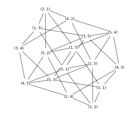
(c) Networkx [20] generated oriented line graph

For instance, consider figure 1(a) which is an arrangement of perfectly reflecting circles in the plane which is often studied in Sinai billiard dynamics [21].This system can be represented as the combinatorial graph depicted in figure 1(b). A billiard can be reflected at any vertex and move towards a neighboring vertex. The movement of billiard over the edge (u,v)(u,v) may be from uu to vv or from vv to uu. Therefore we can define two orientations on every edge. Hence, we find a total 1616 symbols over edges of the above graph mentioned below:

e(1)=(1,2),e(2)=(2,4),e(3)=(4,3),e(4)=(3,1),e(5)=(1,5),e(6)=(2,5),e(7)=(3,5),e(8)=(4,5),\begin{matrix}e^{(1)}=(1,2),&e^{(2)}=(2,4),&e^{(3)}=(4,3),&e^{(4)}=(3,1),\\ e^{(5)}=(1,5),&e^{(6)}=(2,5),&e^{(7)}=(3,5),&e^{(8)}=(4,5),\end{matrix} (48)

and e(8+k)=(e(k))−1e^{(8+k)}=(e^{(k)})^{-1} for k=1,2,…​8k=1,2,\dots 8. The set of all symbols is ℰ={e(k):k=1,2,…16}\mathcal{E}=\{e^{(k)}:k=1,2,\dots 16\}. An example of biinfinite sequence can be given by

W=…​e(1)​e(6)​(e(5))−1​e(1)​e(6)​(e(5))−1​e(1)​e(2)​e(3)​e(7)​(e(8))−1​e(3)​e(7)​(e(8))−1​…=(e(1)​e(6)​(e(5))−1)p1​e(1)​e(2)​(e(3)​e(7)​(e(8))−1)p2​where​p1,p2∈ℕ.\begin{split}W=&\dots e^{(1)}e^{(6)}(e^{(5)})^{-1}e^{(1)}e^{(6)}(e^{(5)})^{-1}e^{(1)}e^{(2)}e^{(3)}e^{(7)}(e^{(8)})^{-1}e^{(3)}e^{(7)}(e^{(8)})^{-1}\dots\\ =&(e^{(1)}e^{(6)}(e^{(5)})^{-1})^{p_{1}}e^{(1)}e^{(2)}(e^{(3)}e^{(7)}(e^{(8)})^{-1})^{p_{2}}~\text{where}~p_{1},p_{2}\in\mathbb{N}.\end{split} (49)

Here W=(P1)p1​Q​(P2)p2W=(P_{1})^{p_{1}}Q(P_{2})^{p_{2}} where P1=e(1)​e(6)​(e(5))−1P_{1}=e^{(1)}e^{(6)}(e^{(5)})^{-1}, P2=e(3)​e(7)​(e(8))−1P_{2}=e^{(3)}e^{(7)}(e^{(8)})^{-1} are two prime cycles and Q=e(1)​e(2)Q=e^{(1)}e^{(2)} is a finite walk. The oriented line graph is depicted in the figure 1(c) which has 1616 nodes.

As the equation (2) and (6) are not calculation friendly, we derive the Ihara zeta function using the Ihara determinant formula, which is

1ζG​(x)=(1−x2)m−n​det(I−A​x+(D−I)​x2),\frac{1}{\zeta_{G}(x)}=(1-x^{2})^{m-n}\det(I-Ax+(D-I)x^{2}), (50)

where 0≤x<1λ0\leq x<\frac{1}{\lambda}, AA, and DD are the adjacency matrix, and degree matrix of graph GG, as well as II is the identity matrix of order nn. The Ihara zeta function for the graph depicted in figure 1(b) is

ζG​(x)=1(1−x2)3​(48​x10+32​x8−32​x7−8​x6−32​x5−4​x4−8​x3+3​x2+1)\zeta_{G}(x)=\frac{1}{\left(1-x^{2}\right)^{3}\left(48x^{10}+32x^{8}-32x^{7}-8x^{6}-32x^{5}-4x^{4}-8x^{3}+3x^{2}+1\right)} (51)

Hence for any probability value pp, we have ζG​(a​pσ)=1A\zeta_{G}(ap^{\sigma})=\frac{1}{A} where

A=(1−a2p2​σ)3[48a10p10​σ+32a8p8​σ−32a7p7​σ−8a6p6​σ−32a5p5​σ−4a4p4​σ−8a3p3​σ+3a2p2​σ+1].\begin{split}A=\left(1-a^{2}p^{2\sigma}\right)^{3}[48a^{10}p^{10\sigma}+32a^{8}p^{8\sigma}-32a^{7}p^{7\sigma}-8a^{6}p^{6\sigma}-32a^{5}p^{5\sigma}&\\ -4a^{4}p^{4\sigma}-8a^{3}p^{3\sigma}+3a^{2}p^{2\sigma}+1]&.\end{split} (52)

Also, for any aa we have

ζG​(a)=1(1−a2)3​(48​a10+32​a8−32​a7−8​a6−32​a5−4​a4−8​a3+3​a2+1).\zeta_{G}(a)=\frac{1}{\left(1-a^{2}\right)^{3}\left(48a^{10}+32a^{8}-32a^{7}-8a^{6}-32a^{5}-4a^{4}-8a^{3}+3a^{2}+1\right)}. (53)

The first derivative

ζG′​(x)=6​x(1−x2)4​(48​x10+32​x8−32​x7−8​x6−32​x5−4​x4−8​x3+3​x2+1)−480​x9+256​x7−224​x6−48​x5−160​x4−16​x3−24​x2+6​x(1−x2)3​(48​x10+32​x8−32​x7−8​x6−32​x5−4​x4−8​x3+3​x2+1)2.\begin{split}\zeta_{G}^{\prime}(x)=&\frac{6x}{\left(1-x^{2}\right)^{4}\left(48x^{10}+32x^{8}-32x^{7}-8x^{6}-32x^{5}-4x^{4}-8x^{3}+3x^{2}+1\right)}\\ &-\frac{480x^{9}+256x^{7}-224x^{6}-48x^{5}-160x^{4}-16x^{3}-24x^{2}+6x}{\left(1-x^{2}\right)^{3}\left(48x^{10}+32x^{8}-32x^{7}-8x^{6}-32x^{5}-4x^{4}-8x^{3}+3x^{2}+1\right)^{2}}.\end{split} (54)

It gives us the expression of 1σ⁡(1−a​ζG′​(a))\frac{1}{\sigma(1-a\zeta_{G}^{\prime}(a))}, where σ⁡(1−a​ζG′​(a))=\sigma(1-a\zeta_{G}^{\prime}(a))=

σ−6​a2​σ(a−1)5​(a+1)4​(2​a2+1)2​(12​a5+12​a4+8​a3−a−1)−2​(120​a6+4​a4−56​a3−14​a2−12​a+3)​a2​σ(a−1)5​(a+1)3​(2​a2+1)3​(−12​a5−12​a4−8​a3+a+1)2\begin{split}\sigma-\frac{6a^{2}\sigma}{(a-1)^{5}(a+1)^{4}\left(2a^{2}+1\right)^{2}\left(12a^{5}+12a^{4}+8a^{3}-a-1\right)}&\\ -\frac{2\left(120a^{6}+4a^{4}-56a^{3}-14a^{2}-12a+3\right)a^{2}\sigma}{(a-1)^{5}(a+1)^{3}\left(2a^{2}+1\right)^{3}\left(-12a^{5}-12a^{4}-8a^{3}+a+1\right)^{2}}&\end{split} (55)

Now for any probability PP we have s⁡(p)=p​ζG​(a​pσ)−ζG​(a)+1−pσσ⁡(1−a​ζG′​(a))=p×ABs(p)=p\frac{\zeta_{G}(ap^{\sigma})-\zeta_{G}(a)+1-p^{\sigma}}{\sigma(1-a\zeta_{G}^{\prime}(a))}=\frac{p\times A}{B} where

A=1−pσ+1(a−1)4​(a+1)3​(2​a2+1)2​(6​a3+a−1)​(2​a​(a+1)+1)−1(a​pσ−1)4​(a​pσ+1)3​(2​a2​p2​σ+1)2​(6​a3​p3​σ+a​pσ−1)​(2​a​pσ​(a​pσ+1)+1)and​B=σ−8​a3​(a⁡(a⁡(2​a​(a⁡(24​a​(a+1)+11)−2)−13)−8)−3)​σ(a−1)5​(a+1)4​(2​a2+1)3​(6​a3+a−1)2​(2​a​(a+1)+1)2.\begin{split}A=1-p^{\sigma}+\frac{1}{(a-1)^{4}(a+1)^{3}\left(2a^{2}+1\right)^{2}\left(6a^{3}+a-1\right)(2a(a+1)+1)}&\\ -\frac{1}{\left(ap^{\sigma}-1\right)^{4}\left(ap^{\sigma}+1\right)^{3}\left(2a^{2}p^{2\sigma}+1\right)^{2}\left(6a^{3}p^{3\sigma}+ap^{\sigma}-1\right)\left(2ap^{\sigma}\left(ap^{\sigma}+1\right)+1\right)}&\\ \text{and}~B=\sigma-\frac{8a^{3}(a(a(2a(a(24a(a+1)+11)-2)-13)-8)-3)\sigma}{(a-1)^{5}(a+1)^{4}\left(2a^{2}+1\right)^{3}\left(6a^{3}+a-1\right)^{2}(2a(a+1)+1)^{2}}.&\end{split} (56)

The Ihara entropy of the billiard system is SG​([𝒫])=∑is⁡(pi)S_{G}([\mathcal{P}])=\sum_{i}s(p_{i}), where 𝒫={pi}i=1W\mathcal{P}=\{p_{i}\}_{i=1}^{W} is any given discrete probability distribution.

Acknowledgement

SD is thankful to his Ph.D. supervisor Dr. Subhashish Banerjee for introducing him with the Ihara Zeta function and its applications in quantum information theory.

References

  • [1] Audrey Terras. Zeta functions of graphs: a stroll through the garden, volume 128. Cambridge University Press, 2010.
  • [2] Yasutaka Ihara. On discrete subgroups of the two by two projective linear group over p-adic fields. Journal of the Mathematical Society of Japan, 18(3):219–235, 1966.
  • [3] P-L Giscard and Paul Rochet. Algebraic combinatorics on trace monoids: extending number theory to walks on graphs. SIAM Journal on Discrete Mathematics, 31(2):1428–1453, 2017.
  • [4] Anton Deitmar. Ihara zeta functions of infinite weighted graphs. SIAM Journal on Discrete Mathematics, 29(4):2100–2116, 2015.
  • [5] Jean A Dieudonne. Introduction to the theory of formal groups, volume 20. CRC Press, 1973.
  • [6] Piergiulio Tempesta. A theorem on the existence of trace-form generalized entropies. Proc. R. Soc. A, 471(2183):20150165, 2015.
  • [7] Piergiulio Tempesta. Beyond the shannon–khinchin formulation: the composability axiom and the universal-group entropy. Annals of Physics, 365:180–197, 2016.
  • [8] Motoko Kotani and Toshikazu Sunada. 2.-zeta functions of finite graphs. Journal of Mathematical Sciences-University of Tokyo, 7(1):7–26, 2000.
  • [9] Andries E Brouwer and Willem H Haemers. Spectra of graphs. Springer Science & Business Media, 2011.
  • [10] Samuel Rota Bulò, Edwin R Hancock, Furqan Aziz, and Marcello Pelillo. Efficient computation of ihara coefficients using the bell polynomial recursion. Linear Algebra and Its Applications, 436(5):1436–1441, 2012.
  • [11] Inverting formal power series wrt. composition. Mathematics Stack Exchange. URL:https://math.stackexchange.com/q/334245 (version: 2013-03-18).
  • [12] Claude E Shannon and Warren Weaver. The mathematical theory of communication. 1949. Urbana, IL: University of Illinois Press, 1963.
  • [13] Claude Elwood Shannon. A mathematical theory of communication. Bell system technical journal, 27(3):379–423, 1948.
  • [14] A Ya Khinchin. Mathematical foundations of information theory. Courier Corporation, 2013.
  • [15] Mark Pollicott. Dynamical zeta functions. In PROCEEDINGS OF SYMPOSIA IN PURE MATHEMATICS, volume 69, pages 409–428. Providence, RI; American Mathematical Society; 1998, 2001.
  • [16] Aleksei Mikhailovich Nikitin. The ihara–selberg zeta function of a finite graph and symbolic dynamics. Algebra i Analiz, 13(5):134–149, 2001.
  • [17] Douglas Lind, Brian Marcus, Lind Douglas, and Marcus Brian. An introduction to symbolic dynamics and coding. Cambridge university press, 1995.
  • [18] Per Dahlqvist. Approximate zeta functions for the sinai billiard and related systems. Nonlinearity, 8(1):11, 1995.
  • [19] Takehiko Morita. The symbolic representation of billiards without boundary condition. Transactions of the American Mathematical Society, 325(2):819–828, 1991.
  • [20] Aric Hagberg, Pieter Swart, and Daniel S Chult. Exploring network structure, dynamics, and function using networkx. Proceedings of the 7th Python in Science Conference (SciPy2008), page 11–15, Aug 2008. (Pasadena, CA USA).
  • [21] Weisstein, Eric W. ”Sinai Billiards.” From MathWorld–A Wolfram Web Resource. http://mathworld.wolfram.com/SinaiBilliards.html.