A neural network based policy iteration algorithm with global -superlinear convergence for stochastic games on domains
Abstract. In this work, we propose a class of numerical schemes for solving semilinear Hamilton-Jacobi-Bellman-Isaacs (HJBI) boundary value problems which arise naturally from exit time problems of diffusion processes with controlled drift. We exploit policy iteration to reduce the semilinear problem into a sequence of linear Dirichlet problems, which are subsequently approximated by a multilayer feedforward neural network ansatz. We establish that the numerical solutions converge globally in the -norm, and further demonstrate that this convergence is superlinear, by interpreting the algorithm as an inexact Newton iteration for the HJBI equation. Moreover, we construct the optimal feedback controls from the numerical value functions and deduce convergence. The numerical schemes and convergence results are then extended to oblique derivative boundary conditions. Numerical experiments on the stochastic Zermelo navigation problem are presented to illustrate the theoretical results and to demonstrate the effectiveness of the method.
Key words. Hamilton-Jacobi-Bellman-Isaacs equations, neural networks, policy iteration, inexact semismooth Newton method, global convergence, -superlinear convergence.
AMS subject classifications. 82C32, 91A15, 65M12
1 Introduction
In this article, we propose a class of numerical schemes for solving Hamilton-Jacobi-Bellman-Isaacs (HJBI) boundary value problems of the following form:
| (1.1) |
where is an open bounded domain, is the (nonconvex) Hamiltonian defined as
| (1.2) |
with given nonempty compact sets , and is a boundary operator, i.e., if is the identity operator, (1.1) is an HJBI Dirichlet problem, while if with some functions , (1.1) is an HJBI oblique derivative problem. Above and hereafter, when there is no ambiguity, we shall adopt the summation convention as in [20], i.e., repeated equal dummy indices indicate summation from to .
It is well-known that the value function of zero-sum stochastic differential games in domains satisfies the HJBI equation (1.1), and the optimal feedback controls can be constructed from the derivatives of the solutions (see e.g. [32] and references within; see also Section 6 for a concrete example). In particular, the HJBI Dirichlet problem corresponds to exit time problems of diffusion processes with controlled drift (see e.g. [32, 10, 37]), while the HJBI oblique derivative problem corresponds to state constraints (see e.g. [36, 34]). A nonconvex HJBI equation as above also arises from a penalty approximation of hybrid control problems involving continous controls, optimal stopping and impulse controls, where the HJB (quasi-)variational inequality can be reduced to an HJBI equation by penalizing the difference between the value function and the obstacles (see e.g. [27, 47, 39, 40]). As (1.1) in general cannot be solved analytically, it is important to construct effective numerical schemes to find the solution of (1.1) and its derivatives.
The standard approach to solving (1.1) is to first discretize the operators in (1.1) by finite difference or finite element methods, and then solve the resulting nonlinear discretized equations by using policy iteration, also known as Howard’s algorithm, or generally (finite-dimensional) semismooth Newton methods (see e.g. [18, 8, 45, 39]). However, this approach has the following drawbacks, as do most mesh-based methods: (1) it can be difficult to generate meshes and to construct consistent numerical schemes for problems in domains with complicated geometries; (2) the number of unknowns in general grows exponentially with the dimension , i.e., it suffers from Bellman’s curse of dimensionality, and hence this approach is infeasible for solving high-dimensional control problems. Moreover, since policy iteration is applied to a fixed finite-dimensional equation resulting from a particular discretization, it is difficult to infer whether the same convergence rate of policy iteration remains valid as the mesh size tends to zero ([42, 8]). We further remark that, for a given discrete HJBI equation, it can be difficult to determine a good initialization of policy iteration to ensure fast convergence of the algorithm; see [2] and references therein on possible accelerated methods.
Recently, numerical methods based on deep neural networks have been designed to solve high-dimensional partial differential equations (PDEs) (see e.g. [35, 15, 6, 16, 26, 44]). Most of these methods reformulate (1.1) into a nonlinear least-squares problem:
| (1.3) |
where is a collection of neural networks with a smooth activation function. Based on collocation points chosen randomly from the domain, (1.3) is then reduced into an empirical risk minimization problem, which is subsequently solved by using stochastic optimization algorithms, in particular the Stochastic Gradient Descent (SGD) algorithm or its variants. Since these methods avoid mesh generation, they can be adapted to solve PDEs in high-dimensional domains with complex geometries. Moreover, the choice of smooth activation functions leads to smooth numerical solutions, whose values can be evaluated everywhere without interpolations. In the following, we shall refer to these methods as the Direct Method, due to the fact that there is no policy iteration involved.
We observe, however, that the Direct Method also has several serious drawbacks, especially for solving nonlinear nonsmooth equations including (1.1). Firstly, the nonconvexity of both the deep neural networks and the Hamiltonian leads to a nonconvex empirical minimization problem, for which there is no theoretical guarantee on the convergence of SGD to a minimizer (see e.g. [43]). In practice, training a network with a desired accuracy could take hours or days (with hundreds of thousands of iterations) due to the slow convergence of SGD. Secondly, each SGD iteration requires the evaluation of (with respect to and ) on sample points, but is not necessarily defined everywhere due to the nonsmoothness of . Moreover, evaluating the function (again on a large set of sample points) can be expensive, especially when the sets A and B are of high dimensions, as we do not require more regularity than continuity of the coefficients with respect to the controls, so that approximate optimization may only be achieved by exhaustive search over a discrete coverage of the compact control set. Finally, as we shall see in Remark 4.2, merely including an -norm of the boundary data in the loss function (1.3) does not generally lead to convergence of the derivatives of numerical solutions or the corresponding feedback control laws.
In this work, we propose an efficient neural network based policy iteration algorithm for solving (1.1). At the th iteration, , we shall update the control laws by performing pointwise maximization/minimization of the Hamiltonian based on the previous iterate , and obtain the next iterate by solving a linear boundary value problem, whose coefficients involve the control laws . This reduces the (nonconvex) semilinear problem into a sequence of linear boundary value problems, which are subsequently approximated by a multilayer neural network ansatz. Note that compared to Algorithm Ho-3 in [8] for discrete HJBI equations, which requires to solve a nonlinear HJB subproblem (involving minimization over the set B) for each iteration, our algorithm only requires to solve a linear subproblem for each iteration, hence it is in general more efficient, especially when the dimension of B is high.
Policy iteration (or Successive Galerkin Approximation) was employed in [4, 5, 28, 30] to solve convex HJB equations on the whole space . Specifically, [4, 5, 28] approximate the solution to each linear equation via a separable polynomial ansatz (without concluding any convergence rate), while [30] assumes each linear equation is solved sufficiently accurately (without specifying a numerical method), and deduces pointwise linear convergence. The continuous policy iteration in [28] has also been applied to solve HJBI equations on in [29], which is a direct extension of Algorithm Ho-3 in [8] and still requires to solve a nonlinear HJB subproblem at each iteration. In this paper, we propose an easily implementable accuracy criterion for the numerical solutions of the linear PDEs which ensures the numerical solutions converge superlinearly in a suitable function space for nonconvex HJBI equations from an arbitrary initial guess.
Our algorithm enjoys the main advantage of the Direct Method, i.e., it is a mesh-free method and can be applied to solve high-dimensional stochastic games. Moreover, by utilizing the superlinear convergence of policy iteration, our algorithm effectively reduces the number of pointwise maximization/minimization over the sets A and B, and significantly reduces the computational cost of the Direct Method, especially for high dimensional control sets. The superlinear convergence of policy iteration also helps eliminate the oscillation caused by SGD, which leads to smoother and more rapidly decaying loss curves in both the training and validation processes (see Figure 7). Our algorithm further allows training of the feedback controls on a separate network architecture from that representing the value function, or adaptively adjusting the architecture of networks for each policy iteration.
A major theoretical contribution of this work is the proof of global superlinear convergence of the policy iteration algorithm for the HJBI equation (1.1) in , which is novel even for HJB equations (i.e., one of the sets A and B is singleton). Although the (local) superlinear convergence of policy iteration for discrete equations has been proved in various works (e.g. [38, 42, 18, 8, 47, 45, 39]), to the best of our knowledge, there is no published work on the superlinear convergence of policy iteration for HJB PDEs in a function space, nor on the global convergence of policy iteration for solving nonconvex HJBI equations.
Moreover, this is the first paper which demonstrates the convergence of neural network based methods for the solutions and their (first and second order) derivatives of nonlinear PDEs with merely measurable coefficients (cf. [22, 23, 26, 44]). We will also prove the pointwise convergence of the numerical solutions and their derivatives, which subsequently enables us to construct the optimal feedback controls from the numerical value functions and deduce convergence.
Let us briefly comment on the main difficulties encountered in studying the convergence of policy iteration for HJBI equations. Recall that at the th iteration, we need to solve a linear boundary value problem, whose coefficients involve the control laws , obtained by performing pointwise maximization/minimization of the Hamiltonian . The uncountability of the state space and the nonconvexity of the Hamiltonian require us to exploit several technical measurable selection arguments to ensure the measurability of the controls , which is essential for the well-definedness of the linear boundary value problems and the algorithm.
Moreover, the nonconvexity of the Hamiltonian prevents us from following the arguments in [42, 18, 8] for discrete HJB equations to establish the global convergence of our inexact policy iteration algorithm for HJBI equations. In fact, a crucial step in the arguments for discrete HJB equations is to use the discrete maximum principle and show the iterates generated by policy iteration converge monotonically with an arbitrary initial guess, which subsequently implies the global convergence of the iterates. However, this monotone convergence is in general false for the iterates generated by the inexact policy iteration algorithm, due to the nonconvexity of the Hamiltonian and the fact that each linear equation is only solved approximately. We shall present a novel analysis technique for establishing the global convergence of our inexact policy iteration algorithm, by interpreting it as a fixed point iteration in .
Finally, we remark that the proof of superlinear convergence of our algorithm is significantly different from the arguments for discrete equations. Instead of working with the sup-norm for (finite-dimensional) discrete equations as in [42, 18, 8, 47, 39], we employ a two-norm framework to establish the generalized differentiability of HJBI operators, where the norm gap is essential as has already been pointed out in [24, 46, 45]. Moreover, by taking advantage of the fact that the Hamiltonian only involves low order terms, we further demonstrate that the inverse of the generalized derivative is uniformly bounded. Furthermore, we include a suitable fractional Sobolev norm of the boundary data in the loss functions used in the training process, which is crucial for the -superlinear convergence of the neural network based policy iteration algorithm.
We organize this paper as follows. Section 2 states the main assumptions and recalls basic results for HJBI Dirichlet problems. In Section 3 we propose a policy iteration scheme for HJBI Dirichlet problems and establish its global superlinear convergence. Then in Section 4, we shall introduce the neural network based policy iteration algorithm, establish its various convergence properties, and construct convergent approximations to optimal feedback controls. We extend the algorithm and convergence results to HJBI oblique derivative problems in Section 5. Numerical examples for two-dimensional stochastic Zermelo navigation problems are presented in Section 6 to confirm the theoretical findings and to illustrate the effectiveness of our algorithms. The Appendix collects some basic results which are used in this article, and gives a proof for the main result on the HJBI oblique derivative problem.
2 HJBI Dirichlet problems
In this section, we introduce the HJBI Dirichlet boundary value problems of our interest, recall the appropriate notion of solutions, and state the main assumptions on its coefficients. We start with several important spaces used frequently throughout this work.
Let and be a bounded domain in , i.e., a bounded open connected subset of with a boundary. For each integer and real with , we denote by the standard Sobolev space of real functions with their weak derivatives of order up to in the Lebesgue space . When , we use to denote . We further denote by and the spaces of traces from and , respectively (see [21, Proposition 1.1.17]), which can be equivalently defined by using the surface measure on the boundaries as follows (see e.g. [19]):
| (2.1) | ||||
We shall consider the following HJBI equation with nonhomogeneous Dirichlet boundary data:
| (2.2a) | ||||
| (2.2b) | ||||
where the nonlinear Hamiltonian is given as in (1.1):
| (2.3) |
Throughout this paper, we shall focus on the strong solution to (2.2), i.e., a twice weakly differentiable function satisfying the HJBI equation (2.2a) almost everywhere in , and the boundary values on will be interpreted as traces of the corresponding Sobolev space. For instance, on in (2.2b) means that the trace of is equal to in , where denotes the trace operator (see [19, Proposition 1.1.17]). See Section 5 for boundary conditions involving the derivatives of solutions.
We now list the main assumptions on the coefficients of (2.2).
H. 1.
Let , be a bounded domain, A be a nonempty finite set, and B be a nonempty compact metric space. Let , satisfy the following ellipticity condition with a constant :
and satisfy that on , and that is continuous, for all and .
As we shall see in Theorem 3.3 and Corollary 3.5, the finiteness of the set A enables us to establish the semismoothness of the HJBI operator (2.2a), whose coefficients involve a general nonlinear dependence on the parameters and . If all coefficients of (2.2a) are in a separable form, i.e., it holds for all that for some functions (e.g. the penalized equation for variational inequalities with bilateral obstacles in [27]), then we can relax the finiteness of A to the same conditions on B.
Finally, in this work we focus on boundary value problems in a domain to simplify the presentation, but the numerical schemes and their convergence analysis can be extended to problems in nonsmooth convex domains with sufficiently regular coefficients (see e.g. [21, 45]).
We end this section by proving the uniqueness of solutions to the Dirichlet problem (2.2) in . The existence of strong solutions shall be established constructively via policy iteration below (see Theorem 3.7).
Proposition 2.1.
Proof.
Let be two strong solutions to (2.2), we consider the following linear homogeneous Dirichlet problem:
| (2.4) |
where we define the following measurable functions: for each ,
with the Hamiltonian defined as in (2.3). Note that the boundedness of coefficients implies that , and . Moreover, one can directly verify that the following inequality holds for all parametrized functions : for all ,
which together with (H.1) leads to the estimate that on the set , and hence we have a.e. . Then, we can deduce from Theorem A.1 that the Dirichlet problem (2.4) admits a unique strong solution and . Since satisfies (2.4) a.e. in and , we see that is a strong solution to (2.4) and hence , which subsequently implies the uniqueness of strong solutions to the Dirichlet problem (2.2). ∎
3 Policy iteration for HJBI Dirichlet problems
In this section, we propose a policy iteration algorithm for solving the Dirichlet problem (2.2). We shall also establish the global superlinear convergence of the algorithm, which subsequently gives a constructive proof for the existence of a strong solution to the Dirichlet problem (2.2).
We start by presenting the policy iteration scheme for the HJBI equations in Algorithm 1, which extends the policy iteration algorithm (or Howard’s algorithm) for discrete HJB equations (see e.g. [18, 8, 39]) to the continuous setting.
- 1.
Choose an initial guess in , and set .
- 2.
Given the iterate , update the following control laws: for all ,
(3.1) (3.2) - 3.
Solve the linear Dirichlet problem for :
(3.3) where for .
- 4.
If , then terminate with outputs and , otherwise increment by one and go to step 2.
The remaining part of this section is devoted to the convergence analysis of Algorithm 1. For notational simplicity, we first introduce two auxiliary functions: for each with , we shall define the following functions
| (3.4) | ||||
| (3.5) |
Note that for all and , by setting , we can see from (3.1) and (3.2) that
| (3.6) |
We then recall several important concepts, which play a pivotal role in our subsequent analysis. The first concept ensures the existence of measurable feedback controls and the well-posedness of Algorithm 1.
Definition 3.1.
Let be a measurable space, and let and be topological spaces. A function is a Carathéodory function if:
- 1.
for each , the function is -measurable, where is the Borel -algebra of the topological space ; and
- 2.
for each , the function is continuous.
Remark 3.1.
It is well-known that if are two complete separable metric spaces, and is a Carathéodory function, then for any given measurable function , the composition function is measurable (see e.g. [3, Lemma 8.2.3]). Since any compact metric space is complete and separable, it is clear that (H.1) implies that the coefficients are Carathéodory functions (with and ). Moreover, one can easily check that both and are Carathéodory functions, i.e., (resp. ) is continuous in (resp. ) and measurable in (see Theorem A.3 for the measurability of in ).
We now recall a generalized differentiability concept for nonsmooth operators between Banach spaces, which is referred as semismoothness in [46] and slant differentiability in [12, 24]. It is well-known (see e.g. [8, 45, 39]) that the HJBI operator in (2.2a) is in general non-Fréchet-differentiable, and this generalized differentiability is essential for showing the superlinear convergence of policy iteration applied to HJBI equations.
Definition 3.2.
Let be defined on a open subset of the Banach space with images in the Banach space . In addition, let be a given a set-valued mapping with nonempty images, i.e., for all . We say is -semismooth in if for any given , we have that is continuous near , and
The set-valued mapping is called a generalized differential of in .
Remark 3.2.
As in [46], we always require that has a nonempty image, and hence the -semismooth of in shall automatically imply that the image of is nonempty on .
Now we are ready to analyze Algorithm 1. We first prove the semismoothness of the Hamiltonian defined as in (2.3), by viewing it as the composition of a pointwise maximum operator and a family of HJB operators parameterized by the control . Moreover, we shall simultaneously establish that, for each iteration, one can select measurable control laws to ensure the measurability of the controlled coefficients in the linear problem (3.3), which is essential for the well-posedness of strong solutions to (3.3), and the well-definedness of Algorithm 1.
The following proposition establishes the semismoothness of a parameterized family of first-order HJB operators, which extends the result for scalar-valued HJB operators in [45]. Moreover, by taking advantage of the fact that the operators involve only first-order derivatives, we are able to establish that they are semismooth from to for some (cf. [45, Theorem 13]), which is essential for the superlinear convergence of Algorithm 1.
Proposition 3.1.
Suppose (H.1) holds. Let be a given constant satisfying if and if , and let be the HJB operator defined by
Then is Lipschitz continuous and -semismooth in with a generalized differential
defined as follows: for any , we have
| (3.7) |
where is any jointly measurable function such that for all and ,
| (3.8) |
Proof.
Since A is a finite set, we shall assume without loss of generality that, the Banach space is endowed with the usual product norm , i.e., for all , . Note that the Sobolev embedding theorem shows that the following injections are continuous: , for all , and , for all . Thus for any given satisfying the conditions in Proposition 3.1, we can find such that the injection is continuous. Then, the boundedness of implies that the mappings and are well-defined, and is Lipschitz continuous.
Now we show that the mapping has a nonempty image from to , where we choose such that the injection is continuous, and naturally extend the operators and from to . For each , we consider the Carathéodory function such that for all , where is defined by (3.5). Theorem A.3 shows there exists a function satisfying (3.8), i.e.,
and is jointly measurable with respect to the product -algebra on . Hence is nonempty for all .
We proceed to show that the operator is in fact -semismooth from to , which implies the desired conclusion due to the continuous embedding . For each , we denote by the -th component of , and by the -th component of . Theorem A.4 and the continuity of in show that for each , the set-valued mapping
is upper hemicontinuous, from which, by following precisely the steps in the arguments for [45, Theorem 13], we can prove that is -semismooth. Then, by using the fact that a direct product of semismooth operators is again semismooth with respect to the direct product of the generalized differentials of the components (see [46, Proposition 3.6]), we can deduce that is semismooth with respect to the generalized differential and finishes the proof. ∎
We then establish the semismoothness of a general pointwise maximum operator, by extending the result in [24] for the max-function .
Proposition 3.2.
Let be a given constant, A be a finite set, and be a bounded subset of . Let be the pointwise maximum operator such that for each ,
| (3.9) |
Then is -semismooth in with a generalized differential
defined as follows: for any , we have
where is any measurable function such that
| (3.10) |
Moreover, is uniformly bounded (in the operator norm) for all .
Proof.
Let the Banach space be endowed with the product norm defined as in the proof of Proposition 3.1. We first show the mappings and are well-defined, has nonempty images, and is uniformly bounded for .
The finiteness of A implies that any can also be viewed as a Carathéodory function . Hence for any given , we can deduce from Theorem A.3 the existence of a measurable function satisfying (3.10). Moreover, for any given measurable function and , the function remains Lebesgue measurable (see Remark 3.1). Then, for any given with , one can easily check that , and , which subsequently implies that and are well-defined, and the image of is nonempty on . Moreover, for any , Hölder’s inequality leads to the following estimate:
which shows that for all .
Now we prove by contradiction that the operator is -semismooth. Suppose there exists a constant and functions such that as , and
| (3.11) |
where for each , is defined with some measurable function . Then, by passing to a subsequence, we may assume that for all , the sequence converges to zero pointwise a.e. in , as .
For notational simplicity, we define for all and . Then for a.e. , we have for all , for all . By using the finiteness of A and the convergence of , it is straightforward to prove by contradiction that for all such , for all large enough .
We now derive an upper bound of the left-hand side of (3.11). For a.e. , we have
from any . Thus, for each , we have for a.e. that,
where, by applying Theorem A.3 twice, we can see that both the set-valued mapping and the function are measurable.
We then introduce the set for each . The measurability of the set-valued mapping implies the associated distance function is a Carathéodory function (see [1, Theorem 18.5]), which subsequently leads to the measurability of for all . Hence we can deduce that
which leads to the following estimate:
where we have used the bounded convergence theorem and the fact that for a.e. , for all large enough . This contradicts to the hypothesis (3.11), and hence finishes our proof. ∎
Now we are ready to conclude the semismoothness of the HJBI operator. Note that the argument in [45] does not apply directly to the HJBI operator, due to the nonconvexity of the Hamiltonian defined as in (2.3).
Theorem 3.3.
Proof.
Note that we can decompose the HJBI operator into , where is the linear operator , is the HJB operator defined in Proposition 3.1, is the pointwise maximum operator defined in Proposition 3.2, and is a constant satisfying if , and if .
Proposition 3.1 shows that is Lipschitz continuous and semismooth with respect to the generalized differential defined by (3.7), while Proposition 3.2 shows that is semismooth with respect to the uniformly bounded generalized differential defined by (3.9). Hence, we know the composed operator is semismooth with respect to the composition of the generalized differentials (see [46, Proposition 3.8]), i.e., for all . Consequently, by using the fact that is Fréchet differentiable with the derivative , we can conclude from Propositions 3.1 and 3.2 that is semismooth on , and that (3.12) is a desired generalized differential of at . ∎
Note that the above characterization of the generalized differential of the HJBI operator involves a jointly measurable function , satisfying (3.8) for all . We now present a technical lemma, which allows us to view the control law in (3.2) as such a feedback control on and .
Lemma 3.4.
Suppose (H.1) holds. Let , be given measurable functions, and be a measurable function such that for all ,
| (3.14) |
Then there exists a jointly measurable function such that for all , and it holds for all and that
| (3.15) |
Proof.
Let be a given measurable function satisfying (3.14) for all (see Remark 3.1 and Theorem A.3 for the existence of such a measurable function). As shown in the proof of Proposition 3.1, there exists a jointly measurable function satisfying the property (3.15) for all . Now suppose that with (see (H.1)), we shall define the function , such that for all ,
The measurability of and the finiteness of A imply that the set is measurable in the product -algebra on , which along with the joint measurability of leads to the joint measurability of the function .
For any given , we have , from which we can deduce from the definition of that for all . Finally, for any given , we shall verify (3.15) for all and . Let be fixed. If , then the fact that and the definition of imply that , which along with (3.14) and shows that (3.15) holds for the point . On the other hand, if , then and satisfies the condition (3.15) due to the selection of . ∎
As a direct consequence of the above extension result, we now present an equivalent characterization of the generalized differential of the HJBI operator.
Corollary 3.5.
Proof.
Let , and let and be given measurable functions satisfying (3.17) (see Remark 3.1 and Theorem A.3 for the existence of such measurable functions). Then by using Lemma 3.4, we know there exists a jointly measurable function such that satisfies (3.8) for all , and for all . Hence we see the linear operator defined in (3.16) is equal to the following operator
which is a generalized differential of the HJBI operator at due to Theorem 3.3. ∎
The above characterization of the generalized differential of the HJBI operator enables us to demonstrate the superlinear convergence of Algorithm 1 by reformulating it as a semismooth Newton method for an operator equation.
Theorem 3.6.
Proof.
Note that the Dirichlet problem (2.2) can be written as an operator equation with the following operator
where is the HJBI operator defined as in (2.2a), and is the trace operator. Moreover, one can directly check that given an iterate , , the next iterate solves the following Dirichlet problem:
with the differential operator defined as in (3.16). Since is -semismooth (see Corollary 3.5) and , we can conclude that Algorithm 1 is in fact a semismooth Newton method for solving the operator equation .
Note that the boundedness of coefficients and the classical theory of elliptic regularity (see Theorem A.1) imply that under condition (H.1), there exists a constant , such that for any and any , the inverse operator is well-defined, and the operator norm is bounded by , uniformly in . Hence one can conclude from [46, Theorem 3.13] (see also Theorem A.5) that the iterates converges superlinearly to in a neighborhood of . ∎
The next theorem strengthens Theorem 3.6, and establishes a novel global convergence result of Algorithm 1 applied to the Dirichlet problem (2.2), which subsequently provides a constructive proof for the existence of solutions to (2.2). The following additional condition is essential for our proof of the global convergence of Algorithm 1:
H. 2.
Let the function in (H.1) be given as: , for all , where is a sufficiently large constant, depending on , , and .
In practice, (H.2) can be satisfied if (2.2) arises from an infinite-horizon stochastic game with a large discount factor (see e.g. [10]), or if (2.2) stems from an implicit (time-)discretization of parabolic HJBI equations with a small time stepsize.
Theorem 3.7.
Proof.
If Algorithm 1 terminates in iteration , we have and , from which, we obtain from the uniqueness of strong solutions to (2.2) (Proposition 2.1) that is the strong solution to the Dirichlet problem (2.2). Hence we shall assume without loss of generality that Algorithm 1 runs infinitely.
We now establish the global convergence of Algorithm 1 by first showing the iterates form a Cauchy sequence in . For each , we deduce from (3.6) and (H.2) that on and
| (3.18) |
for a.e. , where the function for all , and the modified Hamiltonian is defined as:
| (3.19) |
Hence, by taking the difference of equations corresponding to the indices and , one can obtain that
| (3.20) |
for , and on .
It has been proved in Theorem 9.14 of [20] that, there exist positive constants and , depending only on and , such that it holds for all with , and for all that
which, together with the identity that and the boundedness of , implies that the same estimate also holds for :
Thus, by assuming and using the boundedness of the coefficients, we can deduce from (3.20) that
| (3.21) |
for some constant independent of and the index .
Now we apply the following interpolation inequality (see [20, Theorem 7.28]): there exists a constant , such that for all and , we have . Hence, for any given , we have
Then, by taking , , and assuming that satisfies , we can obtain for that
which implies that is a Cauchy sequence with the norm .
We end this section with an important remark that, if one of the sets A and B is a singleton, and for all , then Algorithm 1 applied to the Dirichlet problem (2.2) is in fact monotonically convergent with an arbitrary initial guess. Suppose, for instance, that A is a singleton, then for each , we have that
Hence we can deduce that is a weak subsolution to , i.e.,
Thus, the weak maximal principle (see [19, Theorem 1.3.7]) and the fact that a.e. (with respect to the surface measure), leads to the estimate , which consequently implies that for all and a.e. .
4 Inexact policy iteration for HJBI Dirichlet problems
Note that at each policy iteration, Algorithm 1 requires us to obtain an exact solution to a linear Dirichlet boundary value problem, which is generally infeasible. Moreover, an accurate computation of numerical solutions to linear Dirichlet boundary value problems could be expensive, especially in a high-dimensional setting. In this section, we shall propose an inexact policy iteration algorithm for (2.2), where we compute an approximate solution to (3.3) by solving an optimization problem over a family of trial functions, while maintaining the superlinear convergence of policy iteration.
We shall make the following assumption on the trial functions of the optimization problem.
H. 3.
The collections of trial functions satisfies the following properties: for all , and is dense in .
It is clear that (H.3) is satisfied by any reasonable -conforming finite element spaces (see e.g. [9]) and high-order polynomial spaces or kernel-function spaces used in global spectral methods (see e.g. [4, 5, 13, 28, 29]). We now demonstrate that (H.3) can also be easily satisfied by the sets of multi-layer feedforward neural networks, which provides effective trial functions for high-dimensional problems. Let us first recall the definition of a feedforward neural network.
Definition 4.1 (Artificial neural networks).
Let be given constants, and be a given function. For each , let be an affine function given as for some and . A function defined as
is called a feedforward neural network. Here the activation function is applied componentwise. We shall refer the quantity as the depth of , as the dimensions of the hidden layers, and as the dimensions of the input and output layers, respectively. We also refer to the number of entries of as the complexity of .
Let , be some nondecreasing sequences of natural numbers, we define for each the set of all neural networks with depth , input dimension being equal to , output dimension being equal to 1, and dimensions of hidden layers being equal to . It is clear that if for all , then we have . The following proposition is proved in [25, Corollary 3.8], which shows neural networks with one hidden layer are dense in .
Proposition 4.1.
Let be an open bounded starshaped domain, and satisfying for all . Then the family of all neural networks with depth is dense in .
Now we discuss how to approximate the strong solutions of Dirichlet problems by reformulating the equations into optimization problems over trial functions. The idea is similar to least squares finite-element methods (see e.g. [7]), and has been employed previously to develop numerical methods for PDEs based on neural networks (see e.g. [35, 6, 44]). However, compared to [6, 35], we do not impose additional constraints on the trial functions by requiring that the networks exactly agree with the boundary conditions, due to the lack of theoretical support that the constrained neural networks are still dense in the solution space. Moreover, to ensure the convergence of solutions in the -norm, we include the -norm of the boundary data in the cost function, instead of the -norm used in [44] (see Remark 4.2 for more details).
For each , let be the unique solution to the Dirichlet problem (3.3):
where and denote the linear elliptic operator and the source term in (3.3), respectively. For each , we shall consider the following optimization problems:
| (4.1) |
The following result shows that the cost function provides a computable indicator of the error.
Proposition 4.2.
Proof.
Let and . The definition of implies that , and . Then, by using the assumption that solves (3.3), we deduce that the residual term satisfies the following Dirichlet problem:
Hence the boundedness of coefficients and the regularity theory of elliptic operators (see Theorem A.1) lead to the estimate that
where the constants depend only on the -norms of , which are independent of . The above estimate, together with the facts that is dense in and , leads to the desired result that . ∎
We now present the inexact policy iteration algorithm for the HJBI problem (2.2), where at each policy iteration, we solve the linear Dirichlet problem within a given accuracy.
- 1.
Choose a family of trial functions , an initial guess in , a sequence of positive scalars, and set .
- 2.
- 3.
- 4.
If , then terminate with outputs and , otherwise increment by one and go to step 2.
Remark 4.1.
In practice, the evaluation of the squared residuals in (4.2) depends on the choice of trial functions. For trial functions with linear architecture, e.g. if are finite element spaces, high-order polynomial spaces, and kernel-function spaces (see [9, 13, 28, 29]), one may evaluate the norms by applying high-order quadrature rules to the basis functions involved.
For trial functions with nonlinear architecture, such as feedforward neural networks, we can replace the integrations in by the empirical mean over suitable collocation points in and on , such as pseudorandom points or quasi-Monte Carlo points (see Section 6; see also [35, 6, 44]). In particular, due to the existence of local coordinate charts of the boundaries, we can evaluate the double integral in the definition of the -norm (see (2.1)) by first generating points in and then mapping the samples onto . The resulting empirical least-squares problem for the -th policy iteration step (cf. (4.1)) can then be solved by stochastic gradient descent (SGD) algorithms; see Section 6. We remark that, instead of pre-generating all the collocation points in advance, one can perform gradient descent based on a sequence of mini-batches of points generated at each SGD iteration. This is particularly useful in higher dimensions, where many collocation points may be needed to cover the boundary, and using mini-batches avoids having to evaluate functions at all collocation points in each iteration.
It is well-known (see e.g. [46, 14]) that the residual term is crucial for the superlinear convergence of inexact Newton methods. This next theorem establishes the global superlinear convergence of Algorithm 2.
Theorem 4.3.
Suppose (H.1), (H.2) and (H.3) hold, and in Algorithm 2. Let be the solution to the Dirichlet problem (2.2). Then for any initial guess , Algorithm 2 either terminates with for some , or generates a sequence that converges -superlinearly to in , i.e., . Consequently, we have for a.e. , and for all .
Proof.
Let be an arbitrary initial guess. We first show that Algorithm 2 is always well-defined. For each , if is the strong solution to (3.3), then we can choose , which satisfies (4.2) and terminates the algorithm. If does not solve (3.3), the fact that is dense in enables us to find satisfying the criterion (4.2).
Moreover, one can clearly see from (4.2) that if Algorithm 2 terminates at iteration , then is the exact solution to the Dirichlet problem (2.2). Hence in the sequel we shall assume without loss of generality that Algorithm 2 runs infinitely, i.e., and for all .
We next show the iterates converge to in by following similar arguments as those for Theorem 3.7. For each , we can deduce from (4.2) that there exists and such that
| (4.3) |
and with . Then, by taking the difference between (4.3) and (2.2), we obtain that
and on , where is the modified Hamiltonian defined as in (3.19). Then, by proceeding along the lines of Theorem 3.7, we can obtain a positive constant , independent of and the index , such that
as , where the additional high-order terms are due to the residuals and . Then, by using the interpolation inequality and assuming is sufficiently large, we can deduce that converge linearly to in .
We then reformulate Algorithm 2 into a quasi-Newton method for the operator equation , with the operator defined in the proof of Theorem 3.6. Let denote the strong dual space of , and denote the dual product on . For each , by using the fact that , we can choose satisfying , and introduce the following linear operators and :
Then, we can apply the identity and rewrite (4.3) as:
with as shown in Theorem 3.6. Hence one can clearly see that (4.3) is precisely a Newton step with a perturbed operator for the equation .
Now we are ready to establish the superlinear convergence of . For notational simplicity, in the subsequent analysis we shall denote by the Banach space with the usual product norm for each . By using the semismoothess of (see Theorem 3.6) and the strong convergence of in , we can directly infer from Theorem A.5 that it remains to show that there exists a open neighborhood of , and a constant , such that
| (4.4) |
and also
| (4.5) |
The criterion (4.2) and the definitions of and imply that (4.5) holds:
as . Moreover, the boundedness of the coefficients shows that is Lipschitz continuous. Finally, the characterization of the generalized differential of in Theorem 3.6 and the regularity theory of elliptic operators (see Theorem A.1) show that for each , we can choose an invertible operator such that , uniformly in . Thus we can conclude from the semismoothness of at that
for all in some neighborhood of , which completes our proof for -superlinear convergence of .
Finally, we establish the pointwise convergence of and their derivatives. For any given , the superlinear convergence of implies that there exists a constant , depending on , such that for all . Taking the summation over the index , we have
where we used the monotone convergence theorem in the first equality. Thus, we have
which leads us to the pointwise convergence of and its partial derivatives with respect to . ∎
Remark 4.2.
We reiterate that merely including the -norm of the boundary data in the cost functional (4.2) in general cannot guarantee the convergence of the derivatives of the numerical solutions , which can be seen from the following simple example. Let be a sequence such that in but not in , and for each , let be the strong solution to in and on .
The fact that in implies that in as . We now show in . Let be the solution to in and on , we can deduce from the integration by parts and the a priori estimate that
which shows that as . Now let be a given family of trial functions, which is dense in . One can find satisfying , and consequently in as . However, we have
Similarly, one can construct functions such that as , but does not converge to in .
We end this section with a convergent approximation of the optimal control strategies based on the iterates generated by Algorithm 2. For any given , we denote by and the set of optimal control strategies for all and for a.e. , such that
As an important consequence of the superlinear convergence of Algorithm 2, we now conclude that the feedback control strategies and generated by Algorithm 2 are convergent to the optimal control strategies.
Corollary 4.4.
Suppose the assumptions of Theorem 4.3 hold, and let be the solution to the Dirichlet problem (2.2). Assume further that there exist functions and such that and for a.e. . Then the measurable functions and , , generated by Algorithm 2 converge to the optimal feedback control pointwise almost everywhere.
Proof.
Let and be the Carathéodory functions defined by (3.4) and (3.5), respectively, and we consider the following set-valued mappings:
| (4.6) | ||||
Theorem A.4 implies that the set-valued mappings and are upper hemicontinuous. Then the result follows directly from the pointwise convergence of in Theorem 4.3, and the fact that and are singleton for a.e. . ∎
Remark 4.3.
If we assume in addition that and for some Banach spaces and , then by using the compactness of A and B (see (H.1)), we can conclude from the dominated convergence theorem that in and in , for any .
5 Inexact policy iteration for HJBI oblique derivative problems
In this section, we extend the algorithms introduced in previous sections to more general boundary value problems. In particular, we shall propose a neural network based policy iteration algorithm with global -superlinear convergence for solving HJBI boundary value problems with oblique derivative boundary conditions. Similar arguments can be adapted to design superlinear convergent schemes for mixed boundary value problems with both Dirichlet and oblique derivative boundary conditions.
We consider the following HJBI oblique derivative problem:
| (5.1a) | ||||
| (5.1b) | ||||
where (5.1a) is the HJBI equation given in (2.2a), and (5.1b) is an oblique boundary condition. Note that the boundary condition on involves the traces of and its first partial derivatives, which exist almost everywhere on (with respect to the surface measure).
The following conditions are imposed on the coefficients of (5.1):
H. 4.
Assume , A, B, , satisfy the same conditions as those in (H.1). Let , , on , and assume there exists a constant , such that on , and on , where are the components of the unit outer normal vector field on .
The next proposition establishes the well-posedness of the oblique derivative problem.
Proposition 5.1.
Proof.
We shall establish the uniqueness of strong solutions to (5.1) in this proof, and then explicitly construct the solution in Theorem 5.2 with the help of policy iteration; see also Theorem 3.7. Suppose that are two strong solutions to (5.1), then we can see is a strong solution to the following linear oblique derivative problem:
| (5.2) |
where is defined as in Proposition 2.1, and
By following the same arguments as the proof of Proposition 2.1, we can show that , and a.e. in , which, along with Theorem A.2, implies that is the unique strong solution to (5.2), and consequently in . ∎
Now we present the neural network based policy iteration algorithm for solving the oblique derivative problem and establish its rate of convergence.
- 1.
Choose a family of trial functions , an initial guess in , a sequence of positive scalars, and set .
- 2.
- 3.
- 4.
If , then terminate with outputs and , otherwise increment by one and go to step 2.
Note that the -norm of the boundary term is included in the cost function , instead of the -norm as in Algorithm 2. It is straightforward to see that Algorithm 3 is well-defined under (H.3) and (H.4). In fact, for each , given the iterate , Corollary 3.5 shows that one can select measurable control laws such that the following linear oblique boundary value problem has measurable coefficients:
and hence admits a unique strong solution in (see Theorem A.2). If , then solve the HJBI oblique derivative problem (5.1), and we can select and terminate the algorithm. Otherwise, the facts that and is dense in allows us to choose sufficiently closed to such that the criterion (5.3) is satisfied, and proceed to the next iteration.
The following result is analogue to Theorem 4.3, and shows the global superlinear convergence of Algorithm 3 for solving the oblique derivative problem (5.1). The proof follows precisely the lines given in Theorem 4.3, hence we shall only present the main steps in Appendix B for the reader’s convenience. The convergence of feedback control laws can be concluded similarly to Corollary 4.4 and Remark 4.3.
Theorem 5.2.
Suppose (H.2), (H.3) and (H.4) hold, and in Algorithm 3. Let be the solution to the oblique derivative problem (5.1). Then for any initial guess , Algorithm 3 either terminates with for some , or generates a sequence that converges -superlinearly to in , i.e., . Consequently, we have for a.e. , and for all .
6 Numerical experiments: Zermelo’s Navigation Problem
In this section, we illustrate the theoretical findings and demonstrate the effectiveness of the schemes through numerical experiments. We present a two-dimensional convection-dominated HJBI Dirichlet boundary value problem in an annulus, which is related to stochastic minimum time problems.
In particular, we consider the stochastic Zermelo navigation problem (see e.g. [37]), which is a time-optimal control problem where the objective is to find the optimal trajectories of a ship/aircraft navigating a region of strong winds, modelled by a random vector field. Given a bounded open set and an adaptive control strategy taking values in A, we assume the dynamics of the ship is governed by the following controlled dynamics:
where the drift coefficient is the sum of the velocity of the wind and the relative velocity of the ship, the nondegenerate diffusion coefficient describes a random perturbation of the velocity field of the wind, and is an -dimensional Brownian motion defined on a probability space .
The aim of the controller is to minimize the expected exit time of the region , taking model ambiguity into account in the spirit of [41]. More generally, we consider the following value function:
| (6.1) |
over all admissible choices of , where denotes the first exit time of the controlled dynamics , the functions and denote the running cost and the exit cost, respectively, which indicate the desired destinations, and is a family of absolutely continuous probability measures with respect to with density , where is a predictable process satisfying for all and a given parameter . In other words, we would like to minimize a functional of the trajectory up to the exit time under the worst-case scenario, with uncertainty arising from the unknown law of the random perturbation.
By using the dual representation of and the dynamic programming principle (see e.g. [41, 10]), we can characterize the value function as the unique viscosity solution to an HJBI Dirichlet boundary value problem of the form (2.2). Moreover, under suitable assumptions, one can further show that is the strong (Sobolev) solution to this Dirichlet problem (see e.g. [33]).
For our numerical experiments, we assume that the domain is an annulus, i.e., , the wind blows along the positive -axis with a magnitude :
which decreases in terms of the distance from the bank, and the random perturbation of the wind is given by the constant diffusion coefficient . We also assume that the ship moves with a constant velocity , and the captain can control the boat’s direction instantaneously, which leads to the following dynamics of the boat in the region:
where represents the angle (measured counter-clockwise) between the positive -axis and the direction of the boat. Finally, we assume the exit cost on and on , which represents that the controller prefers to exit the domain through the inner boundary instead of the outer one (see Figure 6). Then the corresponding Dirichlet problem for the value function in (6.1) is given by: on , on , and
| (6.2) |
where and denote the -norm and -norm on , respectively. The optimal feedback control laws can be further computed as
| (6.3) |
where is the strong solution to (6), and is the angle between and the positive direction. Note that the equation (6) is neither convex nor concave in .
![[Uncaptioned image]](1906.02304v3/ship2.png)
6.1 Implementation details
In this section, we discuss the implementation details of Algorithm 2 for solving (6) with multi-layer neural networks (see Definition 4.1) as the trial functions. We shall now introduce the architecture of the neural networks, the involved hyper-parameters, and various computational aspects of the training process.
For simplicity, we shall adopt a fixed set of trial functions for all policy iterations, which contains fully-connected networks with the activation function , the depth , and the dimension of each hidden layer . The hyper-parameters and will be chosen depending on the complexity of the problem, which ensures that admits sufficient flexibility to approximate the solutions within the desired accuracy. More complicated architectures of neural networks with shortcut connections can be adopted to further improve the performance of the algorithm (see e.g. [16, 44]).
We then proceed to discuss the computation of the cost functional in (4.2) for each policy iteration. It is well-known that Sobolev norms of functions on sufficiently smooth boundaries can be explicitly computed via local coordinate charts of the boundaries (see e.g. [21]). In particular, due to the annulus shaped domain and the constant boundary conditions used in our experiment, we can express the cost functional as follows: for all and ,
| (6.4) | ||||
where we define the map for . Note that we introduce an extra weighting parameter in (6.4), which helps achieve the optimal balance between the residual of the PDE and the residuals of the boundary data. We set the parameter for all the computations.
The cost functional (6.4) is further approximated by an empirical cost via the collocation method (see [35, 6]), where we discretize and by sets of collocation points and , respectively, and write the discrete form of (6.4) as follows: for all and ,
| (6.5) | ||||
where , and for are, respectively, the Lebesgue measures of the domain and boundaries. Note that the choice of the smooth activation function implies that every trial function is smooth, hence all its derivatives are well-defined at any given point. For simplicity, we take the same number of collocation points in the domain and on the boundaries, i.e., .
It is clear that the choice of collocation points is crucial for the accuracy and efficiency of the algorithm. Since the total number of points in a regular grid grows exponentially with respect to the dimension, such a construction is infeasible for high-dimensional problems. Moreover, it is well-known that uniformly distributed pseudorandom points in high dimensions tend to cluster on hyperplanes and lead to a suboptimal distribution by relevant measures of uniformity (see e.g. [11, 6]). Therefore, we shall generate collocation points by a quasi-Monte Carlo (QMC) method based on low-discrepancy sequences. In particular, we first define points in from the generalized Halton sequence (see [17]), and then map those points into the annulus via the polar map , where and for all . The above transformation preserves fractional area, which ensures that a set of well-distributed points on the square will map to a set of points spread evenly over the annulus. We also use Halton points to approximate the (one-dimensional) boundary segments.
Now we are ready to describe the training process, i.e., how to optimize (6.5) over all trial functions in . The optimization is performed by using the well-known Adam stochastic gradient descent (SGD) algorithm [31] with a decaying learning rate schedule. At each SGD iteration, we randomly draw a mini-batch of points with size from the collection of collocation points, and perform gradient descent based on these samples. We initialize the learning rate at and decrease it by a factor of for every 2000 SGD iterations for the examples with analytic solutions in Section 6.2, while for the examples without analytic solutions in Section 6.3 we decrease the learning rate by a factor of once the total number of iterations reaches one of the milestones .
We implement Algorithm 2 using PyTorch and perform all computations on a NVIDIA Tesla K40 GPU with 12 GB memory. The entire algorithm can be briefly summarized as follows. Let be a given sequence, denoting the accuracy requirement for each policy iteration. For each , given the previous iterate , we compute the feedback controls as in (6.3) and obtain the controlled coefficients as defined in (3.3). Then we apply the SGD method with analytically derived gradient to optimize over until we obtain a solution satisfying , where denotes the discrete -norm evaluated based on the training samples in . We then proceed to the next policy iteration, and terminate Algorithm 2 once the desired accuracy is achieved.
6.2 Examples with analytical solutions
In this section, we shall examine the convergence of Algorithm 2 for solving Dirichlet problems of the form (6) with known solutions. In particular, we shall choose a running cost such that the analytical solution to (6) is given by for all . To demonstrate the generalizability and the superlinear convergence of the numerical solutions obtained by Algorithm 2, we generate a different set of collocation points in of the size , and use them to estimate the relative error and the -factor of the numerical solution obtained from the -th policy iteration for all :
We use neural networks with depth and varying as trial functions, initialize Algorithm 2 with , and perform experiments with the following model parameters: , , , , , and .


Figure 2 depicts the performance of Algorithm 2 with different sizes of training samples and the dimensions of hidden layers, which are denoted by and respectively. The hyper-parameters are chosen as and for all . One can clearly see from Figure 2 (left) and (middle) that, despite the fact that Algorithm 2 is initialized with a relatively poor initial guess, the numerical solutions converge superlinearly to the exact solution in the -norm for all these combinations of and , which confirms the theoretical result in Theorem 4.3. It is interesting to observe from Figure 2 that, even though increasing either the complexity of the networks (the red lines) or the size of training samples (the black lines) seems to accelerate the training process slightly (right), neither of them ensures a higher generalization accuracy on the testing samples (left). In all our computations, the accuracies of numerical solutions in the -norm and the -norm are in general higher than the accuracy in the -norm. For example, both the -relative error and the -relative error of the numerical solution obtained at the 9th policy iteration with are 0.0045.


We then proceed to analyze the effects of the hyper-parameters . Roughly speaking, the magnitude of indicates the accuracy of the iterates to the linear Dirichlet problems in the initial stage of Algorithm 2, while the decay of determines the speed at which the -factors converge to , at an extra cost of solving the optimization problem in a given iteration more accurately for smaller . Figure 3 presents the numerical results for different choices of with a fixed training sample size , hidden width and for all . Note that solving each linear equation extremely accurate in the initial stage, i.e., by choosing to be a small value (the blue line), may not be beneficial for the overall performance of the algorithm in terms of both the accuracy and computational efficiency. This is due to the fact that the initialization of the algorithm is in general far from the exact solution to the semilinear boundary value problem, and so are the solutions of the linear equations arising from the first few policy iterations. In fact, it appears in our experiments that the choices of lead to the optimal performance of Algorithm 2, which solves the initial equations sufficiently accurately, and leverages the superlinear convergence of policy iteration to achieve a higher accuracy with a similar computational cost.


We further perform computations with different choices of by fixing the training sample size and the hidden width . Numerical results are shown in Figure 4, from which we can clearly observe that the iterates obtained with , , converge more rapidly to the exact solution. Note that for , the optimal performance of the algorithm is achieved at instead of . This is due to the fact that we solve the first linear Dirichlet problem up to the accuracy (if we ignore the requirement that in (4.2)), hence one needs to enlarge for a smaller , such that is of the same magnitude as before. We observe that the rapid convergence of policy iteration indeed improves the efficiency of the algorithm, in the sense that, to achieve the same accuracy, Algorithm 2 with requires slightly less computational time than Algorithm 2 with , even though Algorithm 2 with takes more time to solve the linear equations for each policy iteration; see the last few iterations of the blue line and the black line. This efficiency improvement is more pronounced for the practical problems with complicated solutions in Section 6.3; see Figure 7 and Table 1.
Finally, we shall compare the efficiency of Algorithm 2 (with , ) to that of the Direct Methods (see e.g. [35, 6, 16, 44]) by fixing the trial functions (-layer networks with hidden width ), the training samples (with size ) and the learning rate of the SGD algorithm. In the Direct Methods, we shall directly apply the SGD method to minimize the following (discretized) squared residual of the semilinear boundary value problem (6):22 2 Strictly speaking, the squared residual (6.6) is not differentiable (with respect to the network parameters) at the samples where one of the first partial derivatives of the current iterate is zero, due to the nonsmooth functions in the HJBI operator (see (6)). In practice, PyTorch will assign 0 as partial derivatives of and functions at their nondifferentiable points, and use it in the backward propagation.
| (6.6) |
where is the discrete interior norm evaluated from the training samples in , and is a certain discrete boundary norm evaluated from samples on the boundary. In particular, we shall perform computations by setting (defined as in (6.5)) and with different choices of ( in [44] and in [16]), which will be referred to as “DM with ” and “DM with ”, respectively, in the following discussion. For both the Direct Methods and Algorithm 2, we shall estimate the -relative error of the numerical solution obtained from the -th SGD iteration by using the same testing samples in of the size as follows:
where denotes the analytical solution to (6).
Figure 5 (left) depicts the -convergence of “DM with ” and “DM with ” (with various choices of ) as the number of SGD iterations tends to infinity, which clearly shows that, compared with using the -boundary norm as in [16, 44], incorporating the -boundary norm in the loss function helps achieve a higher -accuracy of the numerical solutions. It is interesting to point out that, even though penalizing the -norm of the boundary term with a suitable parameter helps improve the accuracy of “DM with ” as suggested in [16], in our experiments, leads to the best -convergence of “DM with ” (after SGD iterations) among other choices of .
Figure 5 (right) presents the decay of -relative errors with respect to the number of SGD iterations used in “DM with ”, “DM with ” and Algorithm 2, which clearly demonstrates that the superlinear convergence of policy iteration significantly accelerates the convergence of the algorithm. In particular, the accuracy enhancement of Algorithm 2 over “DM with ” (or equivalently the Deep Galerkin Method proposed in [44]) is of a factor of 20 with SGD iterations. We remark that the training time of Algorithm 2 is only slightly longer than that of “DM with ” (the runtimes of Algorithm 2 and “DM with ” with SGD iterations are 333 and 308 seconds, respectively), since Algorithm 2 requires to determine whether a given iterate solves the policy evaluation equations sufficiently accurate (see (4.2)), in order to proceed to the next policy iteration step.


6.3 Examples without analytical solutions
In this section, we shall demonstrate the performance of Algorithm 2 by solving (6) with . This corresponds to a minimum time problem with preferred targets, whose solution in general is not known analytically. Numerical simulations will be conducted with the following model parameters: , , , , and but two different values of , and , which are associated with the two scenarios where the ship moves slower than and faster than the wind, respectively. The algorithm is initialized with .
We remark that this is a numerically challenging problem due to the fact that the convection term in (6) dominates the diffusion term, which leads to a sharp change of the solution and its derivatives near the boundaries. However, as we shall see, these boundary layers can be captured effectively by the numerical solutions of Algorithm 2.
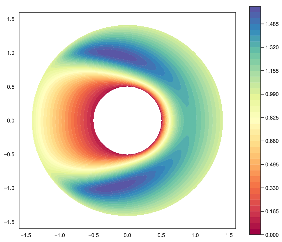
Figure 6 presents the numerical results for the two different scenarios obtained by Algorithm 2 with , and for all . The set of trial functions consists of all fully-connected neural networks with depth and hidden width (the total number of parameters in this network is 12951). We can clearly see from Figure 6 (left) and (middle) that for both scenarios, the numerical solution and its derivatives are symmetric with respect to the axis , and change rapidly near the boundaries.
The feedback control strategies, computed by (6.3), are depicted in Figure 6 (right). If the ship starts from the left-hand side and travels toward the inner boundary, then the expected travel time to is around , which is smaller than the exit cost along . Hence the ship would move in the direction of the positive -axis for both cases, and . However, the optimal control is different for the two scenarios if the ship is on the right-hand side. For the case where the ship’s speed is less than the wind (), if the ship is closed to , then it would move in the direction of the negative -axis, hoping the random perturbation of the wind would bring it to the preferred target, while if it is far from , then it has less chance to reach , so it would move along the positive -axis. On the other hand, for the case where the ship’s speed is larger than the wind (), the ship would in general try to reach the inner boundary. However, if the ship is sufficiently close to in the right-hand half-plane, then the expected travel time to is around , which is larger than the exit cost along . Hence the ship would choose to exit directly from the outer boundary.


We then analyze the convergence of Algorithm 2 by performing computations with 7-layer networks with different hidden width (networks with wider hidden layers are employed such that every linear Dirichlet problem can be solved more accurately) and parameters . For any given iterate , we shall consider the following (squared) residual of the semilinear boundary value problem (6) :
| (6.7) |
which will be evaluated similar to (6.5) based on testing samples in and on of the same size . Figure 7 presents the decay of the residuals in terms of the number of policy iterations, which suggests the -superlinear convergence of the iterates (the -norms of the last iterates for and are 20.3 and 31.8, respectively). Note that the parameter , leads to a slower and more oscillating convergence of the iterates , due to the fact that we apply a mini-batch SGD method to optimize the discrete cost functional for each policy iteration. A faster and smoother convergence can be achieved by choosing a more rapidly decaying .


We further investigate the influence of the parameters on the accuracy and efficiency of Algorithm 2 in detail. Algorithm 2 is carried out with the same trial functions (7-layer networks with hidden width and complexity 32721) but different (we choose different to keep the quantity constant), and the numerical results are summarized in Table 1. One can clearly see that a more rapidly decaying results in a better overall performance (in terms of accuracy and computational time), even though it requires more time to solve the linear equation for each policy iteration. The rapid decay of not only accelerates the superlinear convergence of the iterates , but also helps to eliminate the oscillation caused by the randomness in the SGD algorithm (see Figure 7), which enables us to achieve a higher accuracy with less total computational effort. However, we should keep in mind that smaller means that we need to solve all linear equations with higher accuracy, which subsequently requires more complicated networks and more careful choices of the optimizers for . Therefore, in general, we need to tune the balance between the superlinear convergence rate of policy iteration and the computational costs of the linear solvers, in order to achieve optimal performance of the algorithm.
| PI Itr | HJBI Residual | SGD Itr | Run time | PI Itr | HJBI Residual | SGD Itr | Run time | |
|---|---|---|---|---|---|---|---|---|
| 9 | 0.0466 | 11030 | 922s | 58 | 0.0252 | 32500 | 2729s | |
| 10 | 0.0144 | 20330 | 1710s | 59 | 0.0201 | 39080 | 3275s | |
| 11 | 0.0046 | 45510 | 3820s | 60 | 0.0156 | 45770 | 3836s | |
Finally, we shall compare the performance of Algorithm 2 (with ) and the Direct Method (with in (6.6)) by fixing the trial functions (7-layer networks with hidden width ), the training samples and the learning rates of the SGD algorithms. For both methods, we shall consider the following squared residual for each iterate obtained from the -th SGD iteration (see (6.7)):
Figure 8 (left) presents the decay of the residuals as the number of SGD iterations tends to infinity, which demonstrates the efficiency improvement of Algorithm 2 over the Direct Method. The superlinear convergence of policy iteration helps to provide better initial guesses of the SGD algorithm, which leads to a more rapidly decaying loss curve with smaller noise (on the validation samples); the HJBI residuals obtained in the last 1000 SGD iterations of Algorithm 2 (resp. the Direct Method) oscillates around the value 0.0028 (resp. 0.0144) with a standard derivation 0.00096 (resp. 0.0093).


7 Conclusions
This paper develops a neural network based policy iteration algorithm for solving HJBI boundary value problems arising in stochastic differential games of diffusion processes with controlled drift and state constraints. We establish the -superlinear convergence of the algorithm in with an arbitrary initial guess, and also the pointwise (almost everywhere) convergence of the numerical solutions and their (first and second order) derivatives, which subsequently leads to convergent approximations of optimal feedback controls. The convergence results also hold for general trial functions, including kernel functions and high-order separable polynomials used in global spectral methods. Numerical examples for stochastic Zermelo navigation problems are presented to illustrate the theoretical findings.
To the best of our knowledge, this is the first paper which demonstrates the global superlinear convergence of policy iteration for nonconvex HJBI equations in function spaces, and proposes convergent neural network based numerical methods for solving the solutions of nonlinear boundary value problems and their derivatives. Natural next steps would be to extend the inexact policy iteration algorithm to parabolic HJBI equations, and to employ neural networks with tailored architectures to enhance the efficiency of the algorithm for solving high-dimensional problems.
Appendix A Some fundamental results
Here, we collect some well-known results which are used frequently in the paper.
We start with the well-posedness of strong solutions to Dirichlet boundary value problems. In the sequel, we shall denote by the trace operator.
Theorem A.1.
([19, Theorem 1.2.19]) Let be a bounded domain. Suppose that for all , is in , and are in , satisfying and
| (A.1) |
for some constant . Then for every and , there exists a unique strong solution to the Dirichlet problem
and the following estimate holds with a constant independent of and :
The next theorem shows the well-posedness of oblique boundary value problems.
Theorem A.2.
([19, Theorem 1.2.20]) Let be a bounded domain. Suppose that for all , is in , and are in , satisfying and the uniform elliptic condition (A.1) for some constant .
Assume in addition, that , on , , and on for some constant , where are the components of the unit outer normal vector field on . Then for every and , there exists a unique strong solution to the following oblique derivative problem:
and the following estimate holds with a constant independent of and :
We then recall several important measurability results. The following measurable selection theorem follows from Theorems 18.10 and 18.19 in [1], and ensures the existence of a measurable selector maximizing (or minimizing) a Carathéodory function.
Theorem A.3.
Let a measurable space and be a separable metrizable space. Let be a measurable set-valued mapping with nonempty compact values, and suppose is a Carathéodory function. Define the value function by , and the set-valued map by . Then we have
- 1.
The value function is measurable.
- 2.
The set-valued mapping is measurable, has nonempty and compact values. Moreover, there exists a measurable function satisfying for each .
The following theorem shows the set-valued mapping is upper hemicontinuous.
Theorem A.4.
([1, Theorem 17.31]) Let be topological spaces, be a nonempty compact subset, and be a continuous function. Define the value function by , and the set-valued map by . Then has nonempty and compact values. Moreover, if is Hausdorff, then is upper hemicontinuous, i.e., for every and every neighborhood of , there is a neighborhood of such that implies .
Finally, we present a special case of [14, Theorem 2], which characterizes -superlinear convergence of quasi-Newton methods for a class of semismooth operator-valued equations.
Theorem A.5.
Let be two Banach spaces, and be a given function with a zero . Suppose there exists an open neighborhood of such that is semismooth with a generalized differential in , and there exists a constant such that
For some starting point in , let the sequence satisfy for all , and be generated by the following quasi-Newton method:
where is a sequence of bounded linear operators in . Let be a sequence of generalized differentials of such that for all , and let . Then -superlinearly if and only if and .
Appendix B Proof of Theorem 5.2
Let be an arbitrary initial guess, we shall assume without loss of generality that Algorithm 3 runs infinitely, i.e., and for all .
We first show converges to the unique solution in . For each , we can deduce from (5.3) that there exists and such that
| (B.1) |
and with . Then, we can proceed as in the proof of Theorem 4.3, and conclude that if with a sufficiently large , then converges to the solution of (5.1).
The -superlinear convergence of Algorithm 3 can then be deduced by interpreting the algorithm as a quasi-Newton method for the operator equation , with the operator , where we introduce the Banach space with the usual product norm for each . Since , we can directly infer from Corollary 3.5 that is semismooth in , with a generalized differential for all . Then, for each , by following the same arguments as in Theorem 4.3, we can construct a perturbed operator , such that (B.1) can be equivalently written as with , and , as . Finally, the regularity theory of elliptic oblique derivative problems (see Theorem A.2) shows that is nonsingular for each , and for some constant independent of . Hence we can verify that there exists a neighborhood of and a constant , such that
which allows us to conclude from Theorem A.5 the -superlinear convergence of .
References
- [1] C. D. Aliprantis and K. C. Border, Infinite Dimensional Analysis: A Hitchhiker’s Guide, 3rd ed., Springer-Verlag, Berlin, 2006.
- [2] A. Alla, M. Falcone, and D. Kalise, An efficient policy iteration algorithm for dynamic programming equations, SIAM J. Sci. Comput., 37 (2015), pp. A181–A200,
- [3] J.-P. Aubin and H. Frankowska, Set-Valued Analysis, Birkhäuser, Basel, 1990.
- [4] R. W. Beard, G. N. Saridis, and J. T. Wen, Galerkin approximation of the Generalized Hamilton-Jacobi-Bellman equation, Automatica, (33) 1997, pp. 2159–2177.
- [5] R. W. Beard and T. W. Mclain, Successive Galerkin approximation algorithms for nonlinear optimal and robust control, Internat. J. Control, (71) 1998, pp. 717–743.
- [6] J. Berg and K. Nyström, A unified deep artificial neural network approach to partial differential equations in complex geometries, Neurocomputing, (317) 2018, pp. 28–41.
- [7] P. B. Bochev and M. D. Gunzburger, Least-Squares Finite Element Methods, Springer, New York, 2009.
- [8] O. Bokanowski, S. Maroso, and H. Zidani, Some convergence results for Howard’s algorithm, SIAM J. Numer. Anal., 47 (2009), pp. 3001–3026.
- [9] S. C. Brenner and L. R. Scott, The Mathematical Theory of Finite Element Methods, Springer-Verlag, New York, 1994.
- [10] R. Buckdahn and T. Y. Nie, Generalized Hamilton–Jacobi–Bellman equations with Dirichlet boundary condition and stochastic exit time optimal control problem, SIAM J. Control Optim., 54 (2016), pp. 602–631.
- [11] C. Cervellera and M. Muselli, Deterministic design for neural network learning: An approach based on discrepancy, IEEE Trans. Neural Networks, 15 (2004), pp. 533–544.
- [12] X. Chen, Z. Nashed, and L. Qi, Smoothing methods and semismooth methods for nondifferentiable operator equations, SIAM J. Numer. Anal., 38 (2000), pp. 1200–1216.
- [13] K.C. Cheung, L. Ling, R. Schaback, -convergence of least-squares kernel collocation methods, SIAM J. Numer. Anal. 56 (2018) 614–633.
- [14] A. L. Dontchev, Generalizations of the Dennis-Moré theorem, SIAM J. Optim., 22 (2012), pp. 821–830.
- [15] W. E, J. Han, and A. Jentzen, Deep learning-based numerical methods for high-dimensional parabolic partial differential equations and backward stochastic differential equations, Commun. Math. Stat., 5 (2017), pp. 349–380.
- [16] W. E and B. Yu, The deep Ritz method: a deep learning-based numerical algorithm for solving variational problems, Commun. Math. Stat., 6 (2018), pp. 1–12.
- [17] H. Faure and C. Lemieux, Generalized Halton sequence in 2008: a comparative study, ACM Trans. Model. Comput. Simul., 19 (2009).
- [18] P. Forsyth and G. Labahn, Numerical methods for controlled Hamilton-Jacobi-Bellman PDEs in finance, J. Computational Finance, 11 (2007/2008, Winter), pp. 1–43.
- [19] M. G. Garroni and J. L. Menaldi, Second order elliptic integro-differential problems, Chapman & Hall/CRC, Boca Raton, FL, 2002.
- [20] D. Gilbarg and N. Trudinger, Elliptic Partial Differential Equations of Second Order, 2nd edition, Springer-Verlag, Berlin, New York, 1983.
- [21] E. Grisvard, Elliptic problems in nonsmooth domains, Pitman, Boston, MA, 1985.
- [22] J. Han and W. E, Deep learning approximation for stochastic control problems, preprint, arXiv:1611.07422, 2016.
- [23] J. Han and J. Long, Convergence of the deep BSDE method for coupled FBSDEs, preprint, arXiv:1811.01165v1, 2018.
- [24] M. Hintermüller, K. Ito, and K. Kunisch, The primal-dual active set strategy as a semismooth Newton method, SIAM J. Optim., 13 (2002), pp. 865–888.
- [25] K. Hornik, M. Stinchcombe, and H. White, Universal approximation of an unknown mapping and its derivatives using multilayer feedforward networks, Neural Networks, 3 (1990), pp. 551–560.
- [26] C. Huré, H. Pham, A. Bachouch, and N. Langrené, Deep neural networks algorithms for stochastic control problems on finite horizon, part I: convergence analysis, preprint, arXiv:1812.04300, 2018.
- [27] K. Ito and K. Kunisch, Semismooth Newton methods for variational inequalities of the first kind, M2AN Math. Model. Numer. Anal., 37 (2003), pp. 41–62.
- [28] D. Kalise and K. Kunisch, Polynomial approximation of high-dimensional Hamilton-Jacobi-Bellman equations and applications to feedback control of semilinear parabolic PDEs, SIAM J. Sci. Comput., 40 (2018), A629–A652.
- [29] D. Kalise, S. Kundu, and K. Kunisch, Robust feedback control of nonlinear PDEs by numerical approximation of high-dimensional Hamilton-Jacobi-Isaacs equations, preprint, arXiv:1905.06276, 2019.
- [30] B. Kerimkulov, D. Šiška, and Ł. Szpruch, Exponential convergence and stability of Howard’s policy improvement algorithm for controlled diffusions, preprint, arXiv:1812.07846, 2018.
- [31] D. P. Kingma and J. Ba, Adam: A Method for Stochastic Optimization, CoRR preprint, https://arxiv.org/abs/1412.6980, 2014.
- [32] N. V. Krylov, On the dynamic programming principle for uniformly nondegenerate stochastic differential games in domains and the Isaacs equations, Probab. Theory Related Fields, 158 (2014), pp. 751–783.
- [33] N.V. Krylov, Sobolev and Viscosity Solutions for Fully Nonlinear Elliptic and Parabolic Equations, Mathematical Surveys and Monographs, 233, Amer. Math. Soc., Providence, RI, 2018.
- [34] H. Kushner and P. Dupuis, Numerical Methods for Stochastic Control Problems in Continuous Time, Springer-Verlag, New York, 1991.
- [35] E. Lagaris, A. Likas, and D. I. Fotiadis, Artificial neural networks for solving ordinary and partial differential equations, IEEE Trans. Neural Netw., 9 (1998) pp. 987–1000.
- [36] P.-L. Lions and A.-S. Sznitman, Stochastic differential equations with reflecting boundary conditions, Comm. Pure Appl. Math., 37 (1984) pp. 511– 553.
- [37] P. Mohajerin Esfahani, D. Chatterjee, and J. Lygeros, The stochastic reach-avoid problem and set characterization for diffusions, Automatica, 70 (2016), pp. 43–56.
- [38] M.L. Puterman and S.L. Brumelle, On the convergence of policy iteration in stationary dynamic programming, Math. Oper. Res., 4 (1979), pp. 60–69.
- [39] C. Reisinger and Y. Zhang, A penalty scheme and policy iteration for nonlocal HJB variational inequalities with monotone drivers, preprint, arXiv:1805.06255, 2018.
- [40] C. Reisinger and Y. Zhang, Error estimates of penalty schemes for quasi-variational inequalities arising from impulse control problems, preprint, arXiv:1901.07841, 2019.
- [41] M. Royer, Backward stochastic differential equations with jumps and related non-linear expectations, Stochastic Process. Appl., 116 (2006), pp. 1358–1376.
- [42] M.S. Santos and J. Rust, Convergence properties of policy iteration, SIAM J. Control Optim., 42 (2004), pp. 2094–2115.
- [43] O. Shamir and T. Zhang, Stochastic gradient descent for non-smooth optimization: Convergence results and optimal averaging schemes, in Proceedings of the International Conference on Machine Learning, 2013.
- [44] J. Sirignano and K. Spiliopoulos, DGM: A deep learning algorithm for solving partial differential equations, J. Comput. Phys., 375 (2018), pp. 1339–1364.
- [45] I. Smears and E. Süli, Discontinuous Galerkin finite element approximation of Hamilton-Jacobi-Bellman equations with Cordes coefficients, SIAM J. Numer. Anal., 52 (2014), pp. 993–1016,
- [46] M. Ulbrich, Semismooth Newton Methods for Variational Inequalities and Constrained Optimization Problems in Function Spaces, MOS-SIAM Ser. Optim. 11, SIAM, Philadelphia, 2011.
- [47] J. H. Witte and C. Reisinger, Penalty methods for the solution of discrete HJB equations: Continuous control and obstacle problems, SIAM J. Numer. Anal., 50 (2012), pp. 595–625.