Pseudo-Goldstone dark matter confronts cosmic ray and collider anomalies

Although there is so far no clear evidence for nongravitational interactions of dark matter (DM), it has been suggested that excess of GeV-scale gamma rays from the galactic center (GC), observed by the Fermi-LAT TheFermi-LAT:2015kwa; TheFermi-LAT:2017vmf, could be due to DM annihilations Goodenough:2009gk; Hooper:2010mq; Hooper:2011ti; Hooper:2013rwa; Daylan:2014rsa; Calore:2014xka; Abazajian:2014fta. A leading alternative astrophysical explanation is that the excess comes from an unresolved population of millisecond pulsars or other astrophysical sources Mirabal:2013rba; Calore:2014oga; OLeary:2015qpx; Bartels:2018xom; Brandt:2015ula, although arguments against the pulsar hypothesis have been presented Hooper:2013nhl; Cholis:2014lta; Haggard:2017lyq. Until such possible point sources are resolved, the DM hypothesis remains viable. In particular, ref. Leane:2019xiy has recently called into question claims that the statistical properties of the GeV excess are more consistent with unresolved point sources than with DM annihilations Bartels:2015aea; Lee:2015fea, rekindling the motivation to consider particle physics models for the GC excess.

At the same time, the AMS collaboration obtained the first precise measurement of the spectrum of cosmic ray antiprotons Aguilar:2016kjl. It has been analyzed by numerous groups who find an excess over the expected flux at energies of 10-20 GeV Fujita:2009wk; Bringmann:2014lpa; Cirelli:2014lwa; Hooper:2014ysa; Kohri:2015mga; Cuoco:2016eej; Cui:2016ppb. Intriguingly, this signal can be simultaneously explained with the GC gamma-ray excess by DM annihilating into $b\bar{b}$ Cholis:2019ejx; Lin:2019ljc; Carena:2019pwq. In this paper we propose that both the GC and the $\bar{p}$ excesses can be explained by the annihilation of pseudo-Nambu Goldstone dark matter (pNGB DM).

A natural explanation for why DM ($\chi$) should annihilate mainly into $b\bar{b}$ is the Higgs portal, since $h\to b\bar{b}$ is the dominant decay channel of the Higgs boson. However this tends to be strongly ruled out by direct detection constraints Aprile:2018dbl, because $h$ couples relatively strongly to nucleons Casas:2017jjg. For this reason, singlet scalar DM in the mass range of interest is excluded except for $m_{\chi}\in(55-62.5)$ GeV, just below the Higgs resonance Cline:2013gha; Athron:2017kgt. But for $m_{\chi}<m_{h}/2$, the cross section for $\chi\chi\to b\bar{b}$ at present times is highly suppressed compared to that during the time of freeze-out in the early universe (as we will discuss below), making singlet scalar DM unsuitable for explaining the cosmic ray excesses.

One way of circumventing the direct detection constraints for Higgs portal models is by taking the DM to be fermionic, coupling to $b$ quarks through a pseudoscalar such that DM-nucleon interactions are spin-dependent and velocity-suppressed Ipek:2014gua; Escudero:2016kpw; Abe:2018emu; Boehm:2014hva; Arina:2014yna. Here we will use a different strategy, taking advantage of an approximate symmetry, following refs. Barger:2008jx; Barger:2010yn; Gross:2017dan. There a simple class of models was considered where the required cancellation for direct detection occurs as consequence of a softly broken global U(1) symmetry, rather than through fine tuning. The DM candidate is the pseudo-Nambu Goldstone boson arising from spontaneous breaking of the global U(1) symmetry, with Higgs portal couplings.

In this case, the pNGB retains the feature of being derivatively coupled with other particles. Its interaction with matter is therefore highly suppressed for nonrelativistic DM, as in direct detection experiments. Loop corrections do not have this feature because of the explicit breaking of the global U(1) symmetry. This has been studied in ref. Azevedo:2018exj; Ishiwata:2018sdi, where it was found that loop corrections are nevertheless very small and well within current direct detection bounds.

The pNGB dark matter model is quite economical, with only four free parameters: the DM mass $m_{\chi}$, the mass of its scalar partner (a second Higgs boson $h_{2}$), the mixing angle $\theta$ between $h_{2}$ and the observed Higgs $h_{1}$, and the vacuum expectation value (VEV) $v_{s}$ that spontaneously breaks the U(1) symmetry (or alternatively the quartic coupling $\lambda_{S}$ of the new complex scalar field $S$). In ref. Gross:2017dan, it was shown that one can easily satisfy the requirements of getting the correct relic density, while respecting other constraints like the Higgs invisible width and perturbative unitarity. Moreover, probing the pNGB DM at the LHC has been discussed in ref. Huitu:2018gbc, and further generalizations of the model have been considered Alanne:2018zjm; Karamitros:2019ewv. However its implications for indirect detection have not been considered prior to this work.

A possible bonus of the pNGB DM model is that it can enhance the stability of the Higgs quartic coupling to higher renormalization scales, in contrast to the SM prediction that the Higgs quartic coupling should become negative around $10^{11}\,$GeV Degrassi:2012ry, triggering an instability. This is a consequence of the Higgs portal coupling, that affects the renormalization group evolution of the Higgs quartic coupling Lebedev:2012zw; EliasMiro:2012ay; Khoze:2014xha; Falkowski:2015iwa; Athron:2018ipf. We identify regions of parameter space where the instability can be avoided and the quartic couplings are perturbative up to the Planck scale, while satisfying the relic abundance constraints and accounting for the cosmic ray excesses.

A further set of tentative anomalies has been identified in results coming from the LEP and CMS experiments, that both point to a new Higgs-like particle $h_{2}$ at a mass close to $96\,$GeV. The LEP anomaly is a mild excess $b\bar{b}$ pairs that would arise from decays of $h_{2}$ following $e^{+}e^{-}\to Zh_{2}$ production via Higgs-strahlung Barate:2003sz. At a similar mass, CMS observes a 2.9 $\sigma$ local excess in the diphoton channel, that could come from $gg\to h_{2}\to\gamma\gamma$ CMS:2015ocq; CMS:2017yta; Sirunyan:2018aui. These observations have motivated theorists to propose a number of models Cao:2016uwt; Fox:2017uwr; Haisch:2017gql; Liu:2018xsw; Vega:2018ddp; LiuLiJia:2019kye; Domingo:2018uim; Biekotter:2019kde; Biekotter:2019mib; Biekotter:2017xmf A necessary ingredient of the pNGB DM model is an additional scalar $h_{2}$ that mixes with the SM Higgs, denoted as $h_{1}$. It is possible to take $m_{h_{2}}=96\,$GeV while still being consistent with the cosmic ray excesses. Although the LEP observation could come directly from the pNGB DM setup, given large enough mixing between the two scalars, the CMS excess requires an additional charged and colored scalar $\Phi$ coupling to the singlet. We make a systematic study of the potential for such extensions of the model to simultaneously explain both tentative signals. as well as the collider anomalies. We show that the extended model including the colored scalar provides an additional means of discovering pNGB DM, by its annihilation to monochromatic gamma rays in the galaxy.

The paper is organized as follows. We review the framework of pNGB DM in section II and then show in section III that it can account for the anomalous cosmic ray signals in gamma rays and antiprotons, for DM mass near $m_{\chi}\sim 65\,$GeV, over wide ranges of the other free parameters. In section IV we explore Higgs stability and perturbativity, showing that it can be achieved if $m_{h_{2}}\gtrsim 140\,$GeV. Section V analyzes a broad class of models that can potentially explain the LEP and CMS anomalies, singling out one that is most promising. We summarize and give conclusions in section VI.

We begin by reviewing the particle physics model, which has just one additional complex scalar field $S=(v_{s}+s+i\chi)/\sqrt{2}$ relative to the standard model (SM). The scalar potential is given by

	$\displaystyle\mathcal{V}$	$\displaystyle=-\frac{\mu_{H}^{2}}{2}|H|^{2}+\frac{\lambda_{H}}{2}|H|^{4}-\frac{\mu_{S}^{2}}{2}|S|^{2}+\frac{\lambda_{S}}{2}|S|^{4}$
		$\displaystyle\penalty\ \penalty\ \penalty\ +\lambda_{HS}|H|^{2}|S|^{2}-\frac{m_{\chi}^{2}}{4}\left(S^{2}+{S^{*}}^{2}\right),$		(1)

where the last term explicitly breaks the global U(1) symmetry $S\to e^{i\alpha}S$, giving mass $m_{\chi}$ to the NGB DM candidate $\chi$. This explicit breaking term can be derived from an extended model with gauged $U(1)$ symmetry at high energy scale Gross:2017dan. From the viewpoint of technical naturalness, there is no need for the soft-breaking mass to be small compared to $\mu_{S}^{2}$; moreover the model’s mechanism for suppressing direct detection signals does not require any hierarchy between the two mass scales.

With no loss of generality, $m_{\chi}^{2}$ can be made real-valued by absorbing its phase with a field redefinition of $S$. Then the DM $\chi$ remains stable due to a $\mathbb{Z}_{2}$ symmetry even after $S$ gets its VEV. The field $H$ is the SM Higgs doublet, $H=(0,(v+h)/\sqrt{2})^{T}$. The VEVs $v_{s}$ and $v$ are

$$\left(\begin{array}[]{c}v^{2}\\ v_{s}^{2}\end{array}\right)=\frac{1}{\lambda_{H}\lambda_{S}-\lambda_{HS}^{2}}\left(\begin{array}[]{cc}\lambda_{S}&-\lambda_{HS}\\ -\lambda_{HS}&\lambda_{H}\end{array}\right)\left(\begin{array}[]{c}\mu_{H}^{2}\\ \mu_{S}^{2}+m_{\chi}^{2}\end{array}\right).$$

(2)

The mass matrix for $h$ and $s$ can be written as

$$M^{2}=\left(\begin{array}[]{cc}\lambda_{H}v^{2}&\lambda_{HS}vv_{s}\\ \lambda_{HS}vv_{s}&\lambda_{S}v_{s}^{2}\end{array}\right)\,,$$

(3)

which is diagonalized by the rotation

$$\left(\begin{array}[]{c}h\\ s\end{array}\right)=\left(\begin{array}[]{cc}c_{\theta}&s_{\theta}\\ -s_{\theta}&c_{\theta}\end{array}\right)\left(\begin{array}[]{c}h_{1}\\ h_{2}\end{array}\right),$$

(4)

with $c_{\theta}=\cos\theta$, $s_{\theta}=\sin\theta$, and the mixing angle given by

$$\tan 2\theta=\frac{2\,\lambda_{HS}vv_{s}}{\lambda_{S}v_{s}^{2}-\lambda_{H}v^{2}}\,.$$

(5)

The mass eigenstate $h_{1}$ is identified as the SM-like Higgs boson with mass $m_{h_{1}}=125\penalty\ \mathrm{GeV}$, and $h_{2}$ is a new $CP$-even state. The trilinear couplings of the DM to the $h_{i}$ bosons are expressed in terms of $\theta$ and the masses as

$$\mathcal{V}\supset-\frac{s_{\theta}\,m_{h_{1}}^{2}}{2v_{s}}h_{1}\chi^{2}+\frac{c_{\theta}\,m_{h_{2}}^{2}}{2v_{s}}h_{2}\chi^{2},$$

(6)

while the $h_{i}$ couplings to SM fermions $f$ have the form

$$\mathcal{L}\supset-\frac{m_{f}}{v}\left(c_{\theta}\,h_{1}+s_{\theta}\,h_{2}\right)\overline{f}f\ .$$

(7)

From the structure of Eqs. (6) and (7), one can see that the matrix element for $\chi f\to\chi f$ scattering mediated by $h_{1,2}$ exchange exactly vanishes at zero momentum transfer, which is the key feature for making the model safe from direct detection constraints. On the other hand for the annihilation $\chi\chi\to f\overline{f}$, the cancellation is ineffective as long as $m_{h_{1}}\not\approx m_{h_{2}}$, since the $s$-channel propagator carries significant momentum. The main annihilation channel determining the DM relic abundance is $\chi\chi\to b\overline{b}$ for $5\penalty\ \mathrm{GeV}\lesssim m_{\chi}\lesssim 70\penalty\ \mathrm{GeV}$, covering the mass range that is relevant for the present work.¹¹ 1 See the next section for discussion of the subdominant $\chi\chi\to WW$ annihilation channel. The DM annihilation cross section for $\chi\chi\to b\bar{b}$ is given by

	$\displaystyle\sigma_{b\overline{b}}v_{\rm rel}$	$\displaystyle\approx\frac{c_{\theta}^{2}\,s_{\theta}^{2}\,m_{b}^{2}}{4\pi v^{2}v_{s}^{2}}\left(1-4\frac{m_{b}^{2}}{m_{\chi}^{2}}\right)^{3/2}$		(8)
		$\displaystyle\penalty\ \penalty\ \penalty\ \times\left|\frac{m_{h_{1}}^{2}}{s-m_{h_{1}}^{2}+im_{h_{1}}\Gamma_{h_{1}}}-\frac{m_{h_{2}}^{2}}{s-m_{h_{2}}^{2}+im_{h_{2}}\Gamma_{h_{2}}}\right|^{2},$

where $\sqrt{s}$ is the total DM energy in the center of mass frame, and $\Gamma_{h_{i}}$ is the total decay width of $h_{i}$. For quantitative determination of the DM relic abundance, we use the full thermally averaged annihilation cross section $\langle\sigma v_{\rm rel}\rangle$ computed using MicrOmegas Belanger:2018mqt.

On the other hand for annihilation within our galaxy, Eq. (II) at $s=4m_{\chi}^{2}$ provides a very good approximation in the DM mass region we consider because the DM is very slowly moving, $v\sim 10^{-3}\,c$, and its kinetic energy is much smaller than the Higgs decay width, $(s-4m_{\chi}^{2})/m_{\chi}\sim m_{\chi}v^{2}\ll\Gamma_{h_{i}}$. Therefore the phase space averaging has a negligible effect on Eq. (II) even exactly on the resonance $4m_{\chi}^{2}=m_{h_{i}}^{2}$, and we can use this expression for predicting indirect detection signals.

It is interesting that Eq. (II) can differ significantly from $\langle\sigma_{b\bar{b}}v_{\rm rel}\rangle$ in the early universe near the resonance at $m_{\chi}=m_{h_{i}}/2$ Ibe:2008ye. We illustrate this in figure 1 by plotting the ratio of $\langle\sigma_{b\bar{b}}v_{\rm rel}\rangle$ at late times versus at the time of freezeout as a function of $m_{\chi}$. This shows that the indirect signal is suppressed by orders of magnitude for $m_{\chi}<m_{h}/2$ and motivates our search for models with $m_{\chi}>m_{h}/2$, where the indirect signal is moderately enhanced, but can nevertheless satisfy Fermi dwarf spheroidal constraints Ackermann:2015zua; Drlica-Wagner:2015xua; Ahnen:2016qkx.

If $m_{\chi}<m_{h_{1}}/2\approx 62.5\penalty\ \mathrm{GeV}$, the trilinear coupling in Eq. (6) gives rise to an invisible decay channel for the Higgs boson, $h_{1}\to\chi\chi$, whose partial width is

$$\Gamma_{\rm inv}=\frac{s_{\theta}^{2}\,m_{h_{1}}^{3}}{32\pi\,v_{s}^{2}}\sqrt{1-4\frac{m_{\chi}^{2}}{m_{h_{1}}^{2}}}\ .$$

(9)

The branching ratio for invisible decays is experimentally constrained at the level of $\mathrm{BR}_{\mathrm{inv}}<0.19$ by the CMS Collaboration Sirunyan:2018owy, and $0.26$ by the ATLAS Collaboration Aaboud:2019rtt. Ignoring the phase space suppression (which is valid for $m_{\chi}\lesssim 60\,$GeV), this gives the approximate constraint $s_{\theta}/v_{s}\lesssim 0.2\penalty\ {\rm\,TeV}^{-1}$.

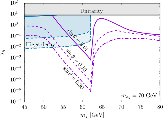
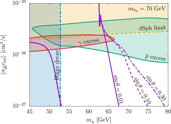
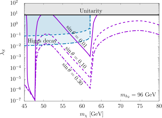
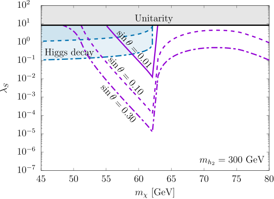
We performed a numerical scan of the parameter space, to look for regions compatible with the gamma-ray and antiproton excesses, as well as DM relic abundance and dwarf spheroidal constraints on DM annihilation. The results are shown in Fig. 2, where the extra Higgs boson mass takes the values $m_{h_{2}}=70,\,96,\,300\penalty\ \mathrm{GeV}$ in successive rows.

In the left panels, the purple lines show the relation between $\lambda_{S}$ and $m_{\chi}$ that gives the correct DM relic abundance, for several values of the mixing angle, $s_{\theta}=0.01$ (solid), $0.10$ (dashed), $0.30$ (dot-dashed). The upper gray and blue regions are excluded by the perturbative unitarity bound $\lambda_{S}<8\pi/3$ Chen:2014ask, and the Higgs invisible decay constraint $\mathrm{BR}_{\mathrm{inv}}<0.19$ Sirunyan:2018owy, respectively. We remark that the relic density curves may be affected by early kinetic decoupling of the DM if its mass is just below the Higgs resonance ($m_{\chi}\lesssim m_{h}/2$) Binder:2017rgn; Duch:2017nbe. As a result, the Higgs invisible decay constraint may change by a factor $\lesssim 7$ Hektor:2019ote. However this does not impact the region of parameter space relevant for explaining the cosmic ray anomalies, so we do not take account of this effect.

In the right panels of Fig. 2, the relic abundance curves (purple) are replotted in the plane of the DM mass and the $s$-wave annihilation cross section, evaluated at the present time, which is relevant for indirect detection. Along each curve, the quartic coupling $\lambda_{S}$ (or equivalently $v_{s}$) is fixed to give the correct relic abundance. To fit the cosmic ray excesses, we adopt the 2$\,\sigma$ allowed regions found in Ref. Cholis:2019ejx, plotted as the red and green regions for the gamma ray and antiproton signals, respectively. For each of the three chosen $m_{h_{2}}$ values, there is some overlap between all the allowed regions, roughly for DM masses in the range $64\penalty\ \mathrm{GeV}\lesssim m_{\chi}\lesssim 67\penalty\ \mathrm{GeV}$. The regions excluded by invisible Higgs decays can be inferred from the corresponding left-hand graph by noticing where the relic density curve goes above the Higgs decay curve for a given mixing angle. It happens that these excluded regions nearly coincide in mass, independently of $\theta$, leading to only a single excluded region in the right-hand plots.

For all but the lowest value of $m_{h_{2}}$, the allowed regions are independent of the mixing angle $\theta$, because only the combination $s_{\theta}/v_{s}$ appears in the $b\overline{b}$ annihilation cross section given by Eq. (II). For $m_{h_{2}}=70$ GeV however, the additional annihilation channel $\chi\chi\to h_{2}h_{2}$ becomes important, breaking this degeneracy. We emphasize that in generic models such as singlet scalar DM, the allowed region for explaining both excesses is excluded by the strong direct detection bound, or suppression of the indirect signal.

The allowed regions are also compatible with the most recent constraints from DM annihilation in satellite galaxies of the Milky Way Fermi-LAT:2016uux; Ando:2016ang, shown in orange. This exclusion is based on gamma-ray observations of 28 confirmed dwarf spheroidal galaxies (dSph) and $17$ new candidate systems, taking advantage of spectroscopically determined $J$-factors for the known dSphs and and predicted $J$-factors for the candidates. It gives a limit that is 1.5 times weaker than in previous determinations.

In our numerical analysis, only the annihilation channel $\chi\chi\to b\overline{b}$ is taken into account for the gamma-ray and antiproton excesses. However for heavy DM, the annihilation into $WW^{*}$ may dominate. We have checked that for $m_{\chi}$ in the range $55\penalty\ \mathrm{GeV}\lesssim m_{\chi}\lesssim 65\penalty\ \mathrm{GeV}$, the branching fraction into $WW^{*}$ can be $25\%$ at most, and the ensuing shapes of the energy spectra of gamma rays and antiprotons are only slightly modified as a result.

Another interesting feature of our model is that the allowed values of the Higgs portal coupling $\lambda_{HS}$ can be compatible with extending the stability of the Higgs potential up to the Planck scale Lebedev:2012zw; EliasMiro:2012ay; Khoze:2014xha; Falkowski:2015iwa; Athron:2018ipf. It is well-established that the Higgs quartic coupling in the SM runs to negative values at high energy scales $\Lambda_{I}\sim 10^{11}$ GeV under renormalization Degrassi:2012ry. This could lead to a catastrophic destabilization of the electroweak vacuum in the early universe, if inflation occurred at a sufficiently high scale East:2016anr.

There are two ways in which the Higgs portal coupling $\lambda_{HS}$ can improve stability. First, it provides an additional positive contribution to the $\beta$ function of $\lambda_{H}$. Second, $\lambda_{H}$ gets a positive threshold correction at the scale $\mu=m_{h_{2}}$ when $h_{2}$ is integrated out. The running $\lambda_{H}$ is increased by $\delta\lambda_{H}\equiv\lambda_{HS}^{2}/\lambda_{S}$ as the scale $\mu$ crosses the threshold from below. For $\lambda_{HS}>0$, the stability condition also becomes more stringent at this scale, $\lambda_{H}>\delta\lambda$ instead of $\lambda_{H}>0$. But as the scale $\mu$ becomes sufficiently large compared to $m_{h_{2}}$, the condition relaxes to the naive requirement $\lambda_{H}(\mu)>0$, so that the threshold correction can overcome the tendency for $\lambda_{H}(\Lambda_{I})$ to become negative. The $\beta$ functions of the couplings at two-loop level are obtained using SARAH Staub:2010jh; Staub:2013tta. Here we concentrate on the $\lambda_{HS}>0$ case since this has been shown to be more effective for Higgs stability than $\lambda_{HS}<0$ EliasMiro:2012ay.

In Fig. 3 we display the regions $\sin\theta$-$\lambda_{S}$ plane that correspond to models with Higgs stability up to the Planck scale (purple region) and that can explain the cosmic ray excesses (red region). The upper plot illustrates the situation for $m_{h_{2}}=300$ GeV. The regions above and to the right of the curves labeled by $\Lambda=10^{5}$, $10^{10}$, $10^{20}$ GeV have a Landau pole in one of the quartic couplings $\lambda_{H}$, $\lambda_{S}$ and $\lambda_{HS}$ at the scale indicated. Thus a fully UV-complete theory can be achieved for parameters in the range $0.1\lesssim\sin\theta\lesssim 0.3$ and $0.06\lesssim\lambda_{S}\lesssim 0.4$. The threshold correction, rather than the extra contribution of $\lambda_{HS}$ to the $\beta$ function, is the most important effect for achieving stability in the overlap region. For $\sin\theta\gtrsim 0.4$, it gives too large an enhancement in $\lambda_{H}$, causing it to blow up at scales $\Lambda$ below the Planck scale; this is the reason the Landau pole curves are vertical at large $\sin\theta$.

In the lower plot of Fig. 3, we show the allowed parameters corresponding to higher values of $m_{h_{2}}$. Here the purple shaded regions combine the requirements of stability of the Higgs potential and perturbativity of the quartic couplings, considering $m_{h_{2}}=300$, $2000$ and $10^{4}$ GeV, requiring smaller $\sin\theta$ with increasing $m_{h_{2}}$. The allowed region for the cosmic ray anomalies shrinks rapidly with increasing $m_{h_{2}}$. For $m_{h_{2}}\gtrsim 600$ GeV, the overlap of the stability and anomaly regions disappears. Moreover for $m_{h_{2}}\lesssim 140\penalty\ \mathrm{GeV}$, there is no longer any region of stability/perturbativity Falkowski:2015iwa.

There are experimental hints for an additional Higgs-like state with mass near 96 GeV. In their search for the SM Higgs, the combined LEP collaborations observed a 2.3 $\sigma$ excess of $b\bar{b}$ final states at $m\sim 98$ GeV, corresponding to a signal strength approximately 10 times lower than would be produced by a SM Higgs of this mass Barate:2003sz.

More recently, in a search for the diphoton final state, CMS reported a 2.9 $\sigma$ (local significance) excess in the 13 TeV data at $m=95.3$ GeV, with a production cross section times branching ratio of $0.13$ pb, close to that which a SM Higgs of the same mass would produce CMS:2015ocq; CMS:2017yta. To simultaneously accommodate both anomalies, we adopt the values taken in ref. Heinemeyer:2018wzl

	$\displaystyle{\sigma(e^{+}e^{-}\to h_{2}\to Zb\bar{b})\over\sigma(e^{+}e^{-}\to h\to Zb\bar{b})}$	$\displaystyle=$	$\displaystyle\mu_{\rm\scriptscriptstyle LEP}=0.117\pm 0.057$
	$\displaystyle{\sigma(gg\to h_{2}\to\gamma\gamma)\over\sigma(gg\to h\to\gamma\gamma)}$	$\displaystyle=$	$\displaystyle\mu_{\rm\scriptscriptstyle CMS}=0.6\pm 0.2$		(10)

where $h$ denotes a SM-like Higgs with mass 96 GeV.

Although the LEP anomaly could be explained by Higgs mixing with angle $\sin\theta\sim\pm\sqrt{0.117}=\pm 0.34$, this would not be sufficient to produce the CMS excess. As pointed out in ref. Fox:2017uwr, one needs to couple $h_{2}$ to new charged states to enhance the branching ratio (by a factor of $\sim 7$) for $h_{2}\to\gamma\gamma$ via the one-loop diagram containing the exotic states.

Annihilation of $\mathcal{O}(60)\penalty\ \mathrm{GeV}$ mass dark matter into $b$ quarks remains as a plausible explanation for excess cosmic gamma-rays and antiprotons that have been observed by Fermi/LAT and AMS respectively. We have shown that an economical model of scalar DM coupling to the Higgs can naturally explain these observations, while respecting other constraints. In particular, the pseudo-Goldstone nature of pNGB DM makes it immune to direct detection, because of its highly velocity-suppressed couplings to nucleons.

We showed that, while firmly within the preferred parameter space for antiprotons, our prediction for the DM mass $m_{\chi}\cong(64-67)\,$GeV is at the high end of the $2\,\sigma$-allowed region for the galactic center gamma-ray excess, and the annihilation cross section is not far below the Fermi indirect detection limit from dwarf spheroidal galaxies. Further, if the extra $CP$-even Higgs boson is in the mass range $m_{h_{2}}\sim(200-600)$ GeV, this allowed region can overlap with parameters for which the Higgs potential remains stable up to the Planck scale, and the new quartic couplings are free from Landau poles.

By extending the model with an additional scalar $\Phi$ that carries charge and color, and assuming that $m_{h_{2}}\sim 96\,$GeV, we can also account for tentative excess $b$ quarks observed at LEP and diphotons at CMS. The most promising such model has $\Phi$ in the $3$ representation, $m_{\Phi}\gtrsim 720\,$GeV, charge $q_{\Phi}=\nicefrac{{8}}{{3}}$, and decaying into four up-type quarks in the first or second generations. It can eventually be ruled out by strengthened limits on pair production of such scalars, or by more precise observations of the production and decay modes of the standard model Higgs boson, with which it has some tensions at the $2\,\sigma$ level. A further test is through the search for a monochromatic gamma-ray line at $\sim 64\,$GeV from the galactic center, which could rule out the extended model with a modest increase in sensitivity over current limits. This extension would require some other new physics to stabilize the Higgs self-coupling and the new scalar cross-couplings at high scales.

Higgs sectors extended by couplings to singlet fields have been invoked to strengthen the electroweak phase transition, possibly enabling electroweak baryogenesis or producing observable gravity waves. This is one feature that the pNGB DM does not have, however, as was shown in ref. Kannike:2019wsn.

This work was supported by the Natural Sciences and Engineering Research Council of Canada (NSERC), Compute Ontario, WestGrid, Compute Canada, and the Yukawa Institute Computer Facility.

References

- (1) M. Ajello et al. [Fermi-LAT Collaboration], “Fermi-LAT Observations of High-Energy -Ray Emission Toward the Galactic Center,” Astrophys. J. 819, no. 1, 44 (2016) [arXiv:1511.02938 [astro-ph.HE]].
- (2) M. Ackermann et al. [Fermi-LAT Collaboration], “The Fermi Galactic Center GeV Excess and Implications for Dark Matter,” Astrophys. J. 840, no. 1, 43 (2017) [arXiv:1704.03910 [astro-ph.HE]].
- (3) L. Goodenough and D. Hooper, “Possible Evidence For Dark Matter Annihilation In The Inner Milky Way From The Fermi Gamma Ray Space Telescope,” arXiv:0910.2998 [hep-ph].
- (4) D. Hooper and L. Goodenough, “Dark Matter Annihilation in The Galactic Center As Seen by the Fermi Gamma Ray Space Telescope,” Phys. Lett. B 697, 412 (2011) [arXiv:1010.2752 [hep-ph]].
- (5) D. Hooper and T. Linden, “On The Origin Of The Gamma Rays From The Galactic Center,” Phys. Rev. D 84, 123005 (2011) [arXiv:1110.0006 [astro-ph.HE]].
- (6) D. Hooper and T. R. Slatyer, “Two Emission Mechanisms in the Fermi Bubbles: A Possible Signal of Annihilating Dark Matter,” Phys. Dark Univ. 2, 118 (2013) [arXiv:1302.6589 [astro-ph.HE]].
- (7) T. Daylan, D. P. Finkbeiner, D. Hooper, T. Linden, S. K. N. Portillo, N. L. Rodd and T. R. Slatyer, “The characterization of the gamma-ray signal from the central Milky Way: A case for annihilating dark matter,” Phys. Dark Univ. 12, 1 (2016) [arXiv:1402.6703 [astro-ph.HE]].
- (8) F. Calore, I. Cholis and C. Weniger, “Background Model Systematics for the Fermi GeV Excess,” JCAP 1503, 038 (2015) [arXiv:1409.0042 [astro-ph.CO]].
- (9) K. N. Abazajian, N. Canac, S. Horiuchi and M. Kaplinghat, “Astrophysical and Dark Matter Interpretations of Extended Gamma-Ray Emission from the Galactic Center,” Phys. Rev. D 90, no. 2, 023526 (2014) [arXiv:1402.4090 [astro-ph.HE]].
- (10) N. Mirabal, “Dark matter vs. Pulsars: Catching the impostor,” Mon. Not. Roy. Astron. Soc. 436, 2461 (2013) [arXiv:1309.3428 [astro-ph.HE]].
- (11) F. Calore, M. D. Mauro and F. Donato, “Diffuse gamma-ray emission from galactic pulsars,” Astrophys. J. 796, 1 (2014) [arXiv:1406.2706 [astro-ph.HE]].
- (12) R. M. O’Leary, M. D. Kistler, M. Kerr and J. Dexter, “Young Pulsars and the Galactic Center GeV Gamma-ray Excess,” arXiv:1504.02477 [astro-ph.HE].
- (13) R. T. Bartels, T. D. P. Edwards and C. Weniger, “Bayesian model comparison and analysis of the Galactic disc population of gamma-ray millisecond pulsars,” Mon. Not. Roy. Astron. Soc. 481, no. 3, 3966 (2018) [arXiv:1805.11097 [astro-ph.HE]].
- (14) T. D. Brandt and B. Kocsis, “Disrupted Globular Clusters Can Explain the Galactic Center Gamma Ray Excess,” Astrophys. J. 812, no. 1, 15 (2015) [arXiv:1507.05616 [astro-ph.HE]].
- (15) D. Hooper, I. Cholis, T. Linden, J. Siegal-Gaskins and T. Slatyer, “Pulsars Cannot Account for the Inner Galaxy’s GeV Excess,” Phys. Rev. D 88, 083009 (2013) [arXiv:1305.0830 [astro-ph.HE]].
- (16) I. Cholis, D. Hooper and T. Linden, “Challenges in Explaining the Galactic Center Gamma-Ray Excess with Millisecond Pulsars,” JCAP 1506, no. 06, 043 (2015) [arXiv:1407.5625 [astro-ph.HE]].
- (17) D. Haggard, C. Heinke, D. Hooper and T. Linden, “Low Mass X-Ray Binaries in the Inner Galaxy: Implications for Millisecond Pulsars and the GeV Excess,” JCAP 1705, 056 (2017) [arXiv:1701.02726 [astro-ph.HE]].
- (18) R. K. Leane and T. R. Slatyer, “Dark Matter Strikes Back at the Galactic Center,” arXiv:1904.08430 [astro-ph.HE].
- (19) R. Bartels, S. Krishnamurthy and C. Weniger, “Strong support for the millisecond pulsar origin of the Galactic center GeV excess,” Phys. Rev. Lett. 116, no. 5, 051102 (2016) [arXiv:1506.05104 [astro-ph.HE]].
- (20) S. K. Lee, M. Lisanti, B. R. Safdi, T. R. Slatyer and W. Xue, “Evidence for Unresolved -Ray Point Sources in the Inner Galaxy,” Phys. Rev. Lett. 116, no. 5, 051103 (2016) [arXiv:1506.05124 [astro-ph.HE]].
- (21) M. Aguilar et al. [AMS Collaboration], “Antiproton Flux, Antiproton-to-Proton Flux Ratio, and Properties of Elementary Particle Fluxes in Primary Cosmic Rays Measured with the Alpha Magnetic Spectrometer on the International Space Station,” Phys. Rev. Lett. 117, no. 9, 091103 (2016).
- (22) Y. Fujita, K. Kohri, R. Yamazaki and K. Ioka, Phys. Rev. D 80, 063003 (2009) [arXiv:0903.5298 [astro-ph.HE]].
- (23) T. Bringmann, M. Vollmann and C. Weniger, “Updated cosmic-ray and radio constraints on light dark matter: Implications for the GeV gamma-ray excess at the Galactic center,” Phys. Rev. D 90, no. 12, 123001 (2014) [arXiv:1406.6027 [astro-ph.HE]].
- (24) M. Cirelli, D. Gaggero, G. Giesen, M. Taoso and A. Urbano, “Antiproton constraints on the GeV gamma-ray excess: a comprehensive analysis,” JCAP 1412, no. 12, 045 (2014) [arXiv:1407.2173 [hep-ph]].
- (25) D. Hooper, T. Linden and P. Mertsch, “What Does The PAMELA Antiproton Spectrum Tell Us About Dark Matter?,” JCAP 1503, no. 03, 021 (2015) [arXiv:1410.1527 [astro-ph.HE]].
- (26) K. Kohri, K. Ioka, Y. Fujita and R. Yamazaki, PTEP 2016, no. 2, 021E01 (2016) [arXiv:1505.01236 [astro-ph.HE]].
- (27) A. Cuoco, M. Krämer and M. Korsmeier, “Novel Dark Matter Constraints from Antiprotons in Light of AMS-02,” Phys. Rev. Lett. 118, no. 19, 191102 (2017) [arXiv:1610.03071 [astro-ph.HE]].
- (28) M. Y. Cui, Q. Yuan, Y. L. S. Tsai and Y. Z. Fan, “Possible dark matter annihilation signal in the AMS-02 antiproton data,” Phys. Rev. Lett. 118, no. 19, 191101 (2017) [arXiv:1610.03840 [astro-ph.HE]].
- (29) I. Cholis, T. Linden and D. Hooper, Phys. Rev. D 99, no. 10, 103026 (2019) [arXiv:1903.02549 [astro-ph.HE]].
- (30) S. J. Lin, X. J. Bi and P. F. Yin, “Investigating the dark matter signal in the cosmic ray antiproton flux with the machine learning method,” arXiv:1903.09545 [astro-ph.HE].
- (31) M. Carena, J. Osborne, N. R. Shah and C. E. M. Wagner, “The Return of the WIMP: Missing Energy Signals and the Galactic Center Excess,” arXiv:1905.03768 [hep-ph].
- (32) E. Aprile et al. [XENON Collaboration], “Dark Matter Search Results from a One Ton-Year Exposure of XENON1T,” Phys. Rev. Lett. 121, no. 11, 111302 (2018) [arXiv:1805.12562 [astro-ph.CO]].
- (33) J. A. Casas, D. G. Cerdeño, J. M. Moreno and J. Quilis, “Reopening the Higgs portal for single scalar dark matter,” JHEP 1705, 036 (2017) [arXiv:1701.08134 [hep-ph]].
- (34) J. M. Cline, K. Kainulainen, P. Scott and C. Weniger, “Update on scalar singlet dark matter,” Phys. Rev. D 88, 055025 (2013) Erratum: [Phys. Rev. D 92, no. 3, 039906 (2015)] [arXiv:1306.4710 [hep-ph]].
- (35) P. Athron et al. [GAMBIT Collaboration], “Status of the scalar singlet dark matter model,” Eur. Phys. J. C 77, no. 8, 568 (2017) [arXiv:1705.07931 [hep-ph]].
- (36) S. Ipek, D. McKeen and A. E. Nelson, “A Renormalizable Model for the Galactic Center Gamma Ray Excess from Dark Matter Annihilation,” Phys. Rev. D 90, no. 5, 055021 (2014) [arXiv:1404.3716 [hep-ph]].
- (37) M. Escudero, D. Hooper and S. J. Witte, “Updated Collider and Direct Detection Constraints on Dark Matter Models for the Galactic Center Gamma-Ray Excess,” JCAP 1702, no. 02, 038 (2017) [arXiv:1612.06462 [hep-ph]].
- (38) T. Abe, M. Fujiwara and J. Hisano, “Loop corrections to dark matter direct detection in a pseudoscalar mediator dark matter model,” JHEP 1902, 028 (2019) [arXiv:1810.01039 [hep-ph]].
- (39) C. Boehm, M. J. Dolan, C. McCabe, M. Spannowsky and C. J. Wallace, “Extended gamma-ray emission from Coy Dark Matter,” JCAP 1405, 009 (2014) [arXiv:1401.6458 [hep-ph]].
- (40) C. Arina, E. Del Nobile and P. Panci, “Dark Matter with Pseudoscalar-Mediated Interactions Explains the DAMA Signal and the Galactic Center Excess,” Phys. Rev. Lett. 114, 011301 (2015) [arXiv:1406.5542 [hep-ph]].
- (41) V. Barger, P. Langacker, M. McCaskey, M. Ramsey-Musolf and G. Shaughnessy, “Complex Singlet Extension of the Standard Model,” Phys. Rev. D 79, 015018 (2009) [arXiv:0811.0393 [hep-ph]].
- (42) V. Barger, M. McCaskey and G. Shaughnessy, “Complex Scalar Dark Matter vis-à-vis CoGeNT, DAMA/LIBRA and XENON100,” Phys. Rev. D 82, 035019 (2010) [arXiv:1005.3328 [hep-ph]].
- (43) C. Gross, O. Lebedev and T. Toma, “Cancellation Mechanism for Dark-Matter-Nucleon Interaction,” Phys. Rev. Lett. 119, no. 19, 191801 (2017) [arXiv:1708.02253 [hep-ph]].
- (44) D. Azevedo, M. Duch, B. Grzadkowski, D. Huang, M. Iglicki and R. Santos, “One-loop contribution to dark-matter-nucleon scattering in the pseudoscalar dark matter model,” JHEP 1901, 138 (2019) [arXiv:1810.06105 [hep-ph]].
- (45) K. Ishiwata and T. Toma, “Probing pseudo Nambu-Goldstone boson dark matter at loop level,” JHEP 1812, 089 (2018) [arXiv:1810.08139 [hep-ph]].
- (46) K. Huitu, N. Koivunen, O. Lebedev, S. Mondal and T. Toma, Phys. Rev. D 100, no. 1, 015009 (2019) [arXiv:1812.05952 [hep-ph]].
- (47) D. Karamitros, Phys. Rev. D 99, no. 9, 095036 (2019) [arXiv:1901.09751 [hep-ph]].
- (48) T. Alanne, M. Heikinheimo, V. Keus, N. Koivunen and K. Tuominen, “Direct and indirect probes of Goldstone dark matter,” Phys. Rev. D 99, no. 7, 075028 (2019) [arXiv:1812.05996 [hep-ph]].
- (49) G. Degrassi, S. Di Vita, J. Elias-Miro, J. R. Espinosa, G. F. Giudice, G. Isidori and A. Strumia, “Higgs mass and vacuum stability in the Standard Model at NNLO,” JHEP 1208, 098 (2012) [arXiv:1205.6497 [hep-ph]].
- (50) O. Lebedev, “On Stability of the Electroweak Vacuum and the Higgs Portal,” Eur. Phys. J. C 72, 2058 (2012) [arXiv:1203.0156 [hep-ph]].
- (51) J. Elias-Miro, J. R. Espinosa, G. F. Giudice, H. M. Lee and A. Strumia, “Stabilization of the Electroweak Vacuum by a Scalar Threshold Effect,” JHEP 1206, 031 (2012) [arXiv:1203.0237 [hep-ph]].
- (52) V. V. Khoze, C. McCabe and G. Ro, “Higgs vacuum stability from the dark matter portal,” JHEP 1408, 026 (2014) [arXiv:1403.4953 [hep-ph]].
- (53) A. Falkowski, C. Gross and O. Lebedev, “A second Higgs from the Higgs portal,” JHEP 1505, 057 (2015) [arXiv:1502.01361 [hep-ph]].
- (54) P. Athron, J. M. Cornell, F. Kahlhoefer, J. Mckay, P. Scott and S. Wild, “Impact of vacuum stability, perturbativity and XENON1T on global fits of and scalar singlet dark matter,” Eur. Phys. J. C 78, no. 10, 830 (2018) [arXiv:1806.11281 [hep-ph]].
- (55) R. Barate et al. [ALEPH and DELPHI and L3 and OPAL Collaborations and LEP Working Group for Higgs boson searches], “Search for the standard model Higgs boson at LEP,” Phys. Lett. B 565, 61 (2003) [hep-ex/0306033].
- (56) CMS Collaboration [CMS Collaboration], “Search for new resonances in the diphoton final state in the mass range between 80 and 115 GeV in pp collisions at TeV,” CMS-PAS-HIG-14-037.
- (57) CMS Collaboration [CMS Collaboration], “Search for new resonances in the diphoton final state in the mass range between 70 and 110 GeV in pp collisions at 8 and 13 TeV,” CMS-PAS-HIG-17-013.
- (58) A. M. Sirunyan et al. [CMS Collaboration], “Search for a standard model-like Higgs boson in the mass range between 70 and 110 GeV in the diphoton final state in proton-proton collisions at 8 and 13 TeV,” Phys. Lett. B 793, 320 (2019) [arXiv:1811.08459 [hep-ex]].
- (59) J. Cao, X. Guo, Y. He, P. Wu and Y. Zhang, “Diphoton signal of the light Higgs boson in natural NMSSM,” Phys. Rev. D 95, no. 11, 116001 (2017) [arXiv:1612.08522 [hep-ph]].
- (60) P. J. Fox and N. Weiner, “Light Signals from a Lighter Higgs,” JHEP 1808, 025 (2018) [arXiv:1710.07649 [hep-ph]].
- (61) U. Haisch and A. Malinauskas, “Let there be light from a second light Higgs doublet,” JHEP 1803, 135 (2018) [arXiv:1712.06599 [hep-ph]].
- (62) D. Liu, J. Liu, C. E. M. Wagner and X. P. Wang, “A Light Higgs at the LHC and the B-Anomalies,” JHEP 1806, 150 (2018) [arXiv:1805.01476 [hep-ph]].
- (63) R. Vega, R. Vega-Morales and K. Xie, “Light (and darkness) from a light hidden Higgs,” JHEP 1806, 137 (2018) [arXiv:1805.01970 [hep-ph]].
- (64) L. Liu, H. Qiao, K. Wang and J. Zhu, “A Light Scalar in the Minimal Dilaton Model in Light of LHC Constraints,” Chin. Phys. C 43, no. 2, 023104 (2019) [arXiv:1812.00107 [hep-ph]].
- (65) T. Biekötter, S. Heinemeyer and C. Muoz, “Precise prediction for the Higgs-boson masses in the SSM,” Eur. Phys. J. C 78, no. 6, 504 (2018) [arXiv:1712.07475 [hep-ph]].
- (66) F. Domingo, S. Heinemeyer, S. Paehr and G. Weiglein, “Decays of the neutral Higgs bosons into SM fermions and gauge bosons in the -violating NMSSM,” Eur. Phys. J. C 78, no. 11, 942 (2018) [arXiv:1807.06322 [hep-ph]].
- (67) T. Biekötter, M. Chakraborti and S. Heinemeyer, “A 96 GeV Higgs Boson in the N2HDM,” arXiv:1903.11661 [hep-ph].
- (68) T. Biekötter, M. Chakraborti and S. Heinemeyer, “An N2HDM Solution for the possible 96 GeV Excess,” arXiv:1905.03280 [hep-ph].
- (69) G. Bélanger, F. Boudjema, A. Goudelis, A. Pukhov and B. Zaldivar, “micrOMEGAs5.0 : Freeze-in,” Comput. Phys. Commun. 231, 173 (2018) [arXiv:1801.03509 [hep-ph]].
- (70) M. Ibe, H. Murayama and T. T. Yanagida, “Breit-Wigner Enhancement of Dark Matter Annihilation,” Phys. Rev. D 79, 095009 (2009) [arXiv:0812.0072 [hep-ph]].
- (71) M. Ackermann et al. [Fermi-LAT Collaboration], “Searching for Dark Matter Annihilation from Milky Way Dwarf Spheroidal Galaxies with Six Years of Fermi Large Area Telescope Data,” Phys. Rev. Lett. 115, no. 23, 231301 (2015) [arXiv:1503.02641 [astro-ph.HE]].
- (72) A. Drlica-Wagner et al. [Fermi-LAT and DES Collaborations], “Search for Gamma-Ray Emission from DES Dwarf Spheroidal Galaxy Candidates with Fermi-LAT Data,” Astrophys. J. 809, no. 1, L4 (2015) [arXiv:1503.02632 [astro-ph.HE]].
- (73) M. L. Ahnen et al. [MAGIC and Fermi-LAT Collaborations], “Limits to Dark Matter Annihilation Cross-Section from a Combined Analysis of MAGIC and Fermi-LAT Observations of Dwarf Satellite Galaxies,” JCAP 1602, no. 02, 039 (2016) [arXiv:1601.06590 [astro-ph.HE]].
- (74) A. M. Sirunyan et al. [CMS Collaboration], Phys. Lett. B 793, 520 (2019) [arXiv:1809.05937 [hep-ex]].
- (75) M. Aaboud et al. [ATLAS Collaboration], Phys. Rev. Lett. 122, no. 23, 231801 (2019) [arXiv:1904.05105 [hep-ex]].
- (76) C. Y. Chen, S. Dawson and I. M. Lewis, “Exploring resonant di-Higgs boson production in the Higgs singlet model,” Phys. Rev. D 91, no. 3, 035015 (2015) [arXiv:1410.5488 [hep-ph]].
- (77) T. Binder, T. Bringmann, M. Gustafsson and A. Hryczuk, Phys. Rev. D 96, no. 11, 115010 (2017) [arXiv:1706.07433 [astro-ph.CO]].
- (78) M. Duch and B. Grzadkowski, JHEP 1709, 159 (2017) [arXiv:1705.10777 [hep-ph]].
- (79) A. Hektor, A. Hryczuk and K. Kannike, JHEP 1903, 204 (2019) [arXiv:1901.08074 [hep-ph]].
- (80) S. Ando and K. Ishiwata, JCAP 1606, no. 06, 045 (2016) [arXiv:1604.02263 [hep-ph]].
- (81) A. Albert et al. [Fermi-LAT and DES Collaborations], “Searching for Dark Matter Annihilation in Recently Discovered Milky Way Satellites with Fermi-LAT,” Astrophys. J. 834, no. 2, 110 (2017) [arXiv:1611.03184 [astro-ph.HE]].
- (82) W. E. East, J. Kearney, B. Shakya, H. Yoo and K. M. Zurek, “Spacetime Dynamics of a Higgs Vacuum Instability During Inflation,” Phys. Rev. D 95, no. 2, 023526 (2017) [Phys. Rev. D 95, 023526 (2017)] [arXiv:1607.00381 [hep-ph]].
- (83) F. Staub, “Automatic Calculation of supersymmetric Renormalization Group Equations and Self Energies,” Comput. Phys. Commun. 182, 808 (2011) [arXiv:1002.0840 [hep-ph]].
- (84) F. Staub, “SARAH 4 : A tool for (not only SUSY) model builders,” Comput. Phys. Commun. 185, 1773 (2014) [arXiv:1309.7223 [hep-ph]].
- (85) S. Heinemeyer and T. Stefaniak, “A Higgs Boson at 96 GeV?!,” PoS CHARGED 2018, 016 (2019) [arXiv:1812.05864 [hep-ph]].
- (86) A. M. Sirunyan et al. [CMS Collaboration], “Search for pair-produced resonances each decaying into at least four quarks in proton-proton collisions at 13 TeV,” Phys. Rev. Lett. 121, no. 14, 141802 (2018) [arXiv:1806.01058 [hep-ex]].
- (87) M. Aaboud et al. [ATLAS Collaboration], “A search for pair-produced resonances in four-jet final states at 13 TeV with the ATLAS detector,” Eur. Phys. J. C 78, no. 3, 250 (2018) [arXiv:1710.07171 [hep-ex]].
- (88) V. Khachatryan et al. [CMS Collaboration], “Search for long-lived charged particles in proton-proton collisions at 13 TeV,” Phys. Rev. D 94, no. 11, 112004 (2016) [arXiv:1609.08382 [hep-ex]].
- (89) A. M. Sirunyan et al. [CMS Collaboration], “Search for pair-produced resonances decaying to quark pairs in proton-proton collisions at 13 TeV,” Phys. Rev. D 98, no. 11, 112014 (2018) [arXiv:1808.03124 [hep-ex]].
- (90) K. Nakamura, K. Nishiwaki, K. y. Oda, S. C. Park and Y. Yamamoto, “Di-higgs enhancement by neutral scalar as probe of new colored sector,” Eur. Phys. J. C 77, no. 5, 273 (2017) [arXiv:1701.06137 [hep-ph]].
- (91) The ATLAS collaboration [ATLAS Collaboration], “Combined measurements of Higgs boson production and decay using up to fb-1 of proton–proton collision data at 13 TeV collected with the ATLAS experiment,” ATLAS-CONF-2019-005.
- (92) A. M. Sirunyan et al. [CMS Collaboration], “Combined measurements of Higgs boson couplings in proton-proton collisions at 13 TeV,” Eur. Phys. J. C 79, 421 (2019) [arXiv:1809.10733 [hep-ex]].
- (93) W. Beenakker, R. Hopker, M. Spira and P. M. Zerwas, “Gluino pair production at the Tevatron,” Z. Phys. C 69, 163 (1995) [hep-ph/9505416].
- (94) C. R. Chen, W. Klemm, V. Rentala and K. Wang, “Color Sextet Scalars at the CERN Large Hadron Collider,” Phys. Rev. D 79, 054002 (2009) [arXiv:0811.2105 [hep-ph]].
- (95) A. D. Martin, W. J. Stirling, R. S. Thorne and G. Watt, “Parton distributions for the LHC,” Eur. Phys. J. C 63, 189 (2009) [arXiv:0901.0002 [hep-ph]].
- (96) V. Khachatryan et al. [CMS Collaboration], “Search for pair-produced resonances decaying to jet pairs in proton-proton collisions at 8 TeV,” Phys. Lett. B 747, 98 (2015) [arXiv:1412.7706 [hep-ex]].
- (97) V. Veeraraghavan [ATLAS Collaboration], “A search for R-parity violating decays of the top squark in four-jet final states with the ATLAS experiment at TeV,” PoS LHCP 2016, 235 (2016).
- (98) The ATLAS collaboration, “Search for Supersymmetry in events with -tagged jets and missing transverse energy in collisions at TeV with the ATLAS detector,” ATLAS-CONF-2017-038.
- (99) CMS Collaboration [CMS Collaboration], “Measurements of Higgs boson production via gluon fusion and vector boson fusion in the diphoton decay channel at TeV,” CMS-PAS-HIG-18-029.
- (100) CMS Collaboration [CMS Collaboration], “Measurements of properties of the Higgs boson in the four-lepton final state in proton-proton collisions at ,” CMS-PAS-HIG-19-001.
- (101) M. Ackermann et al. [Fermi-LAT Collaboration], “Updated search for spectral lines from Galactic dark matter interactions with pass 8 data from the Fermi Large Area Telescope,” Phys. Rev. D 91, no. 12, 122002 (2015) [arXiv:1506.00013 [astro-ph.HE]].
- (102) J. M. Cline, “130 GeV dark matter and the Fermi gamma-ray line,” Phys. Rev. D 86, 015016 (2012) [arXiv:1205.2688 [hep-ph]].
- (103) A. M. Galper et al., Phys. Atom. Nucl. 80, no. 6, 1141 (2017) [Yad. Fiz. 80, no. 6, 660 (2017)].
- (104) K. Kannike and M. Raidal, Phys. Rev. D 99, no. 11, 115010 (2019) [arXiv:1901.03333 [hep-ph]].