Competitive Exclusion in a DAE Model for Microbial Electrolysis Cells
Abstract
Microbial electrolysis cells (MECs) are devices that employ electroactive bacteria to perform extracellular electron transfer, enabling hydrogen generation from biodegradable substrates. In our previous work, we developed and analyzed a differential-algebraic equation (DAE) model for MECs. The model resembles a chemostat or continuous stirred tank reactor (CSTR). Equations are ordinary differential equations (ODEs) for concentrations of substrate, microorganisms, and an extracellular mediator involved in electron transfer. There is also an algebraic constraint for electric current and hydrogen production. Our goal is to determine the outcome of competition between methanogenic archaea and electroactive bacteria, because only the latter contribute to electric current and the resulting hydrogen production. We investigate asymptotic stability in two industrially relevant versions of the model. An important aspect of many chemostat models is the principle of competitive exclusion. This states that only microbes which grow at the lowest substrate concentration will survive as . We show that if methanogens can grow at the lowest substrate concentration, then the equilibrium corresponding to competitive exclusion by methanogens is globally asymptotically stable. The analogous result for electroactive bacteria is not necessarily true. In fact we show that local asymptotic stability of competitive exclusion by electroactive bacteria is not guaranteed, even in a simplified version of the model. In this case, even if electroactive bacteria can grow at the lowest substrate concentration, a few additional conditions are required to guarantee local asymptotic stability. We also provide numerical simulations supporting these arguments. Our results suggest operating conditions that are most conducive to success of electroactive bacteria and the resulting current and hydrogen production in MECs. This will help identify when methane production or electricity and hydrogen production are favored.
keywords
Microbial electrolysis; Competitive exclusion; Asymptotic stability; Differential-algebraic equation;LaSalle’s invariance principle.
1 Introduction
Microbial electrolysis cells (MECs) are an emerging technology that employs microorganisms to recover energy and resources from organic waste [1]. Bacteria on an electroactive anode biofilm oxidize biodegradable substrate and transfer electrons, thereby generating electrical current and releasing protons (H+) [2]. The protons then recombine to form hydrogen at the cathode. A small voltage (0.2–0.8 V) is needed to overcome the thermodynamic barrier, which is much lower than traditional water electrolysis (1.8–3.5 V) and can be supplied by a small solar panel, low-grade heat, or microbial fuel cells (MFCs), all of which can be available onsite [1, 2]. The gap of energy input between microbial and pure electrochemical electrolysis is provided by chemical energy stored in the organics. While the electroactive bacteria facilitate hydrogen production, methanogenic archaea consume the same substrate to produce methane, a product which is less energy efficient [3]. As a result, methanogenesis leads to decreased efficiency of the system. MEC technology has several advantages over other resource recovery and hydrogen production methods. Microbial electrolysis reduces energy use compared to water splitting because some of the energy is derived from embedded energy in the waste biomass [4]. MECs are also more efficient than other methods using renewable wastewater, such as fermentative hydrogen production [5]. In fact, [6] demonstrated up to 96% recovery of the maximum theoretical yield of hydrogen in MECs operated using fermentation effluent.
In our previous work [7], we analyzed and validated a regular, semi-explicit, index 1 differential-algebraic equation (DAE) model for a single substrate MEC [8]. The DAE system is an extended version of an ordinary differential equation (ODE) model for chemostats, also known as continuous stirred tank reactors (CSTRs). Besides an ODE system that describes the rate of change of concentrations of the microorganism populations, the biodegradable substrate, and an extracellular mediator involved in electron transfer, the system also includes an algebraic constraint that relates electric current through the external circuit to the concentrations of the electroactive bacteria and the mediator molecule. This constraint accounts for voltage losses that occur in practice. This construct had been used previously [8] to completely avoid solving Maxwell’s equations in a partial differential equation model. It is also commonly used in chemical fuel cell models [9]. Our group demonstrated computationally that transcritical bifurcations in the dilution rate determine whether electroactive bacteria or methanogens or both will survive at the stable equilibria [7]. The outcome of competition for substrate is a key question because the types of microbes that exist at the system’s stable equilibria determine the electric current and hydrogen production rate. Hydrogen production at the stable equilibrium is possible only if electroactive bacteria are present to generate the needed current. Our efforts here provide answers by characterizing stability of equilibria for two versions of the MEC model, without reference to specific parameter values.
Our goal is to build upon extensive mathematical literature on chemostats to characterize stability of equilibria in the MEC model. One of the main conclusions in the chemostat literature is that if one or more microbes can grow at a lower substrate concentration than the others, then there is a globally asymptotically stable equilibrium where only those microbes have nonzero concentration. This phenomenon is often referred to as competitive exclusion and it holds under a variety of model assumptions. Unfortunately, the MEC analysis is complicated by the fact that growth of the mixed culture bacteria is a nonlinear function of two interdependent variables, the concentrations of both substrate and mediator molecules. In spite of this, we demonstrate that competitive exclusion by methanogens is globally asymptotically stable and provide additional conditions which are necessary for local asymptotic stability of competitive exclusion by electroactive bacteria. The latter suggests that the conditions for competitive exclusion by electroactive bacteria are not as straightforward.
1.1 Model
Versions of the semi-explicit index 1 DAE model for the MEC have been described previously in [7, 8, 10]. Our model differs from [8] by not including fermenting microorganisms that convert a complex substrate into a single compound such as acetate. Competition among fermenting microbes is separate from competition among electroactive bacteria and methanogens and is not a factor in a single simple substrate MEC. Additionally, this model does not include a separate methanogen only biofilm layer on the anode. We consider the following system, extended to include finitely many microbes of each type:
| (1) | ||||
| (2) | ||||
| (3) | ||||
| (4) | ||||
| (5) |
with initial conditions , , , , and . The differential equations represent concentrations, so we are only interested in solutions with nonnegative concentrations. We assume that initial substrate concentration, , is less than or equal to the influent concentration, , and that initial current, , is positive, due to the nonzero electroactive bacteria concentration and a startup period. All of the model parameters are positive.
A single substrate with concentration flows into the tank at constant rate , where is the flow rate per volume and is the fixed influent substrate concentration. Let , and represent the concentrations of microorganisms. The anodic biofilm contains methanogen species with concentrations for , and electroactive bacteria species with concentrations for . Substrate consumption is proportional to monotonically increasing microbial growth rates, or , with constants of proportionality or , respectively. Each microbe also has a constant decay rate, or .
While methanogens only consume the substrate, electroactive bacteria also consume the oxidized form of a mediator molecule, , that is involved in electron transfer. The mediator exists in oxidized and reduced forms, and , respectively. The mediator has a constant maximum concentration, , Following [10], electroactive bacteria are assumed to transfer electrons via oxidation reduction reactions of the form
| (6) | |||
| (7) |
These reactions are represented in the diagram in Figure 1. The oxidized mediator is replenished at a rate proportional to the electric current in the device, , as the reduced mediator molecules transfer electrons to the anode. is the mediator yield of the reactions (6) and (7).
The electric current is related to hydrogen production [7]. This current can be determined by accounting for the voltage losses in the system. Microbial electrolysis is endothermic, so some small external voltage, , is required. The applied voltage may be opposed by some counter-electromotive force, . There are also several sources of voltage losses that occur in practice. Ohmic losses, , arise from various types of resistance in the circuit. Activation losses, , arise from the activation energy of the oxidation-reduction reactions occurring in the cell. Concentration losses, , arise from certain processes that limit the concentration of reactants at the anode and the cathode [9, 11]. All of this can be expressed in the following electrochemical balance equation,
| (8) |
where subscripts A and C represent the anode and cathode, respectively. Previous models have ignored concentration losses at the cathode, , because hydrogen molecules should diffuse away from the cathode rapidly. They have also neglected activation losses at the anode, , under the assumption that the MEC operates with higher voltage losses at the cathode. However, these voltage losses could be included by the general constraint in Section 3. Ohmic losses can be calculated from Ohm’s law, where is the internal resistance. is a decreasing function of the total electroactive bacteria population because less electroactive bacteria is effectively greater resistance in the circuit. Also, with maximum resistance when there are no electroactive bacteria. Following [12], concentration losses at the anode are modeled by the Nernst equation,
| (9) |
where is the ideal gas constant, is the temperature, is the number of moles of electrons transferred per mole of mediator, and is Faraday’s constant. Equation (9) assumes that the reference reduced mediator concentration is equal to the total extracellular mediator concentration, [8, 10]. Activation losses at the cathode are calculated using an approximation to the Butler-Volmer equation for the relationship between electric current and potential at an electrode [8]. Standard simplifying assumptions are that the reaction occurs in one step and that the symmetry coefficient (or the fraction of activation loss that affects the rate of electrochemical transformation) is . With these assumptions we can write
| (10) |
where is the anode surface area and is the reference exchange current density. See [13] for a discussion of approximations to the Butler-Volmer equation.
The following section discusses previous work that has characterized the equilibria of ODE systems resembling equations (1) - (2) when , , and . This paper extends some of those results to analyze local asymptotic stability in a DAE system with additional equations (3) - (5), representing current production by electroactive bacteria bacteria using an extracellular mediator.
1.2 Mathematical Background
There is a large body of literature proving that competitive exclusion occurs for ODE models resembling equations (1) - (2) with , , and . Essentially, stable equilibria may exhibit either competitive exclusion (one species remains), coexistence (multiple species remain), or total extinction (no species remain). Competitive exclusion is generic because coexistence requires multiple species to share an identical parameter value and extinction requires all species to be inadequate competitors. [14] proved the competitive exclusion principle for an ODE model of chemostats with microbial growth determined by Monod kinetics. [15] then provided a more elegant proof using a Lyapunov function to guarantee global stability. These papers showed that, if survival was possible at all, only the microorganism(s) that could grow at the lowest substrate concentration would survive at the stable equilibria. The work also showed that coexistence was only possible if multiple species could grow at the same smallest substrate concentration. [16] provided experiments verifying the theory of competitive exclusion. Subsequently, dozens of authors have proven competitive exclusion occurs in chemostats with various special assumptions. See the monograph [17] or the more recent paper [18] for more details. Besides microbial growth determined by Monod kinetics, we will also clarify our results by focusing on a simplified case of general monotonically increasing growth rates with equal washout rates and a general constraint [19].
To explain microbial electrolysis, the DAE model includes a differential equation for an extracellular mediator involved in electron transfer to the anode as well as an algebraic constraint that determines the electric current. The constraint turns this model into a regular, semi-explicit, index 1 DAE system which does not fit into the previous ODE frameworks. In particular, the constraint (5) used in [7, 8] requires a local representation; global results may not be possible unless the electric current constraint can be solved globally for the electrical current, . In this paper, we extend results from the chemostat literature [15, 19] to analyze local asymptotic stability in the DAE system given by (1) - (5). The following section provides an overview of the structure of the rest of the paper.
1.3 Overview
Section 2 reviews asymptotic stability in semi-explicit DAEs, which is essential to the analysis in the following sections. In particular, we review the relationship between local asymptotic stablility and the spectrum of the matrix pencil, as well as LaSalle’s invariance principle for global stability. In Section 3, we use the spectrum of the matrix pencil of the DAE to characterize local asymptotic stability of equilibria in a simplified model with 1 species of each type, general monotonically increasing kinetics, equal decay rates, and a general constraint. This reveals that competitive exclusion by electroactive bacteria is not locally asymptotically stable unless the spectrum of the matrix pencil satisfies certain conditions. Section 4 proves that competitive exclusion by methanogens is globally asymptotically stable for the full MEC system (1) - (5) with multiplicative Monod kinetics, different decay rates, and a constraint based on the Nernst and Butler-Volmer equations. However, the corresponding result for electroactive bacteria is not likely to be true, as illustrated in the simple case in Section 3. Numerical simulations supporting Theorem 8 and Corollary 9 are provided in Section 5. The conclusion in Section 6 summarizes results and points out that the conditions in Section 3 can be used to evaluate numerically whether competitive exclusion by electroactive bacteria will be locally asymptotically stable or not. The conclusion also indicates that MEC operators will want to avoid operating conditions where methanogens can survive at the lowest substrate value because those conditions make competitive exclusion by methanogens globally asymptotically stable.
2 Asymptotic stability in semi-explicit DAEs
Before presenting results on asymptotic stability of MEC equilibria corresponding to extinction and competitive exclusion, we will briefly review methods for determining asymptotic stability in DAEs [20, 21]. The DAE framework is necessary because the constraint (5) does not admit a global solution. The MEC system in equations (1) - (5) can be represented as a semi-explicit DAE,
| (11) |
where and . More generally, (11) can be viewed as a quasilinear DAE,
| (12) |
where and . Both of these perspectives will be useful. For quasilinear DAEs (12), local asymptotic stability of equilibria can be determined from the spectrum of the matrix pencil, [21, 22, 23, 24]. An equilibrium point of a regular DAE is asymptotically stable if for all elements in [21]. In the following section, we will use the spectrum of the matrix pencil to analyze local asymptotic stability in a simplified model with 1 species of each type, general monotone kinetics, equal decay rates, and a general constraint. The analysis shows that competitive exclusion by methanogens is locally asymptotitcally stable, but the corresponding result is not necessarily true for competitive exclusion by electroactive bacteria.
In the following, we assume that there is some open connected set on which and are twice continuously differentiable, and is nonsingular on .
Condition 1.
Suppose that, for some open, connected set , the following assumptions hold:
- 1.
;
- 2.
is nonsingular on .
Points where is nonsingular are called regular. Under the assumption of nonsingularity of on all of , (11) is a regular DAE, with index 1. By Condition 1, the implicit function theorem allows one to describe as on some open neighborhood of in , where is twice continuously differentiable. At least locally near , dynamics of the differential -variables can be described by a reduced ODE,
| (13) |
Solutions of (13) which satisfy the constraint, , are solutions of the semi-explicit DAE (11) [20, 21].
We will also use the following version of LaSalle’s Invariance principle [25] to analyze global asymptotic stability. A well known property of regular semi-explicit, index 1 DAEs (11) is that they define a smooth vector field on a smooth manifold [21].
Theorem 2 (LaSalle’s invariance principle).
Consider the smooth dynamical system on an manifold given by and let be a compact set in the manifold that is (positively) invariant under the flow of . Let , , be a function such that
in . Let be the largest invariant set in where . Then every solution with initial point in tends asymptotically to as . In particular, if is an isolated equilibrium, it is asymptotically stable.
The function in Theorem 2 is called a Lyapunov function because LaSalle’s theorem generalizes one due to Lyapunov where must be strictly less than zero. Section 4 applies a Lyapunov function modified from [15] to the semi-explicit DAE with finitely many species, multiplicative Monod kinetics, different decay rates, and a constraint that is solvable on .
3 Local asymptotic stability in a simplified model
In this section, we consider local asymptotic stability of equilibrium points corresponding to extinction and competitive exclusion in a simplified MEC model. In contrast to chemostats, competitive exclusion by electroactive bacteria is not necessarily locally asymptotically stable, even when electroactive bacteria can grow at the lowest substrate concentration. This is due to several issues, including the nonlinear dependence of the growth of electroactive bacteria on both mediator and substrate concentrations, as well as the form of the algebraic constraint which determines the electric current. We present this analysis to promote clarity in in Section 4.
Here we simplify the model by assuming that there is one compartment for each type of microbe (i.e., ), that the biofilm decay rates are equal to the dilution rate (i.e., ). We allow for general monotonically increasing kinetics with and . We also allow for a general constraint, , with certain reasonable derivative conditions summarized below. These assumptions allow concise conditions for local asymptotic stability. The presentation of results is simplified if we rescale the model variables. We set
This yields a system of the form
| (14) | ||||
| (15) | ||||
| (16) | ||||
| (17) | ||||
| (18) |
where
and represents the rescaled constraint. Derivatives are taken with respect to rescaled time . Note that we can form the new variable to obtain the system
Since must satisfy , solutions of will approach as . Therefore, any asymptotically stable equilibria will satisfy . We focus on equilibria corresponding to extinction, where , and competitive exclusion, where either or .
In this section, we will allow for general monotonically increasing growth functions and a general constraint. We consider a class of kinetics where the growth rates and substrate consumption rates of the microbes will increase with substrate concentration and also mediator concentration in the case of electroactive bacteria. We require that attainable equilibria exist. We also make several physically reasonable assumptions based on (5). These assumptions state that ohmic voltage losses in will decrease with (because a decrease in electroactive bacteria concentration is effectively an increase in resistance in the circuit), concentration losses will increase with the oxidized mediator as the reduced mediator becomes limited at the anode, and that activation losses will increase with . Additionally, the absence of electroactive bacteria means that no electric current is present. Finally we require unique solutions to at two points. The requirements are summarized by the following condition.
Condition 3.
The kinetics and constraint in this section satisfy:
- 1.
;
- 2.
and are continuously differentiable and monotonically increasing;
- 3.
and such that and for some ;
- 4.
and ;
- 5.
;
- 6.
a unique positive such that ;
- 7.
a unique positive such that .
The rescaled model (14) - (18) has several important equilibrium points corresponding to extinction of all microbes or competitive exclusion by one type of microbe. These depend on the substrate (and mediator) values where each microbe attains zero net growth. and are the substrate concentrations where and , respectively. In the case of the electroactive bacteria, there is a curve that satisfies . In Section 4, Figure 2 depicts what the curve would look like for a system with multiplicative Monod kinetics. Biologically meaningful solutions will be located in the interval , which corresponds to attainable substrate concentrations. If , , then no microbe can ever have positive net growth and if , then all microbes require more substrate than is available given the influent substrate concentration. The model equilibria exhibiting extinction and competitive exclusion are shown in Table 1. The mediator concentrations in these equilibria are the solutions to the constraint, , at the corresponding points. In particular, is the unique positive solution to and is the unique positive solution to .
| Equilibrium Point | Biological Meaning |
|---|---|
| Extinction of all microbes | |
| Competitive exclusion by Methanogens | |
| Competitive exclusion by Electroactive |
The following mutually exclusive cases make one of the equilibrium points locally asymptotically stable. In the final case, local asymptotic stability of the electroactive-only equilibrium also depends on a discriminant that appears in two elements of the spectrum of the matrix pencil at ; we denote this discriminant by
| (19) |
where .
- 1.
(Total Extinction): If , then is locally asymptotically stable.
- 2.
(Competitive Exclusion by Methanogens): If , then is locally asymptotically stable.
- 3.
(Competitive Exclusion by Electroactive): If , and either (1) or (2) , then is locally asymptotically stable.
The extinction equilibrium, , will be unstable in general because we expect at least one microbe to be an adequate competitor with a value in . The spectrum of the matrix pencil at is
so is unstable as long as either or are in the interval . In this case, a microbe introduced into the system may grow in the presence of plentiful substrate. If the methanogen can grow at the lowest substrate value, then the corresponding methanogen-only equilibrium, , will be locally asymptotically stable. The spectrum of the matrix pencil at is
If Case 2 holds, then only will be able to attain positive net growth near the corresponding equilibrium. Finally, the spectrum of the matrix pencil at is where
If Case 3 holds, then is locally asymptotically stable.
Cases 1 - 3 provide conditions for local asymptotic stability of each of the equilibria points and . These apply for any continuously differentiable and monotonically increasing growth functions and and any that satisfies Condition 3. The conditions in Cases 1 - 3 can be checked numerically to determine if a parametrized model permits a locally asymptotically stable equilibrium where only the most competitive electroactive species persists. Unlike the methanogen-only equilibria, local asymptotic stability of the electroactive-only equilibria is not guaranteed when the electroactive bacteria can survive at the lowest substrate value. This means it is unlikely that chemostat results extend to electroactive-only equilibria in an MEC. However, we can assert that for Monod kinetics with different decay rates and a constraint based on the Nernst and Butler-Volmer equations, methanogen-only equilibria are globally asymptotically stable when methanogens can grow at the lowest substrate concentration. The proof of this assertion in Section 4 relies on LaSalle’s invariance principle.
4 Global asymptotic stability with Monod kinetics
In this section, we consider the full MEC system (1) - (5) with multiplicative Monod kinetics, different decay rates, and a constraint based on the Nernst and Butler-Volmer equations. LaSalle’s invariance principle allows us to show that competitive exclusion by methanogens is globally asymptotically stable. The proof uses a Lyapunov function adapted from [15]. Suppose that growth rates for the methanogens are
| (20) |
and growth rates for the electroactive bacteria are
| (21) |
and are the maximum growth rates; and , are half rate constants for consumption of substrate; is the half rate constant for consumption of mediator. As before, the equilibria depend on parameters or functions that are the solutions to and . Denote these solutions by
| (22) | ||||
| (23) |
Assuming that the microbe concentrations are not zero, then and are the substrate concentrations at which each microbe has zero net growth. The difference between the two types of microorganisms is that each electroactive bacteria has zero net growth on a curve . Examples of these curves are shown in Figure 4. The fact that electroactive bacteria have dual substrate-mediator limitation complicates the type of analysis that has appeared in the chemostat literature.
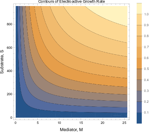


The equilibrium points corresponding to extinction and competitive exclusion in the full unscaled model are given in Table 2. Microbe concentrations at these equilibria are solutions to where only one microbe survives. If or are the most competitive microbes, i.e., or are the smallest values, then equilibrium concentrations are
The mediator concentrations and are the solutions to the constraint (5) at the corresponding points:
Finally, in the case of competitive exclusion by electroactive bacteria, the electric current is the solution to when and :
| Equilibrium Point | Biological Meaning |
|---|---|
| Extinction of all microbe species | |
| Competitive exclusion by methanogen | |
| Competitive exclusion by electroactive bacteria |
This analysis focuses on several sets of interest. Let
| (24) | ||||
In practice, is bounded because the dynamical system is dissipative, as shown in appendix A. The maximum concentration of each microbe must be bounded because it is not biologically possible to have infinite concentration. Although the upper bound for each microbe concentration is not clear, concentrations of each species will be bounded as . Let be the bounded set containing these dynamics. Let be the closed set where the constraint (5) is satisfied. To obtain consistent initial conditions for the DAE, we will assume or the remainder of this section that initial conditions lie in the compact set .
Condition 4.
Suppose that .
Our first theorem relies on the following lemma regarding positivity and boundedness of the DAE solutions.
We defer the proof of Lemma 5 to appendix A. Lemma 5 will be used in the proofs of the theorem later in this section. The next lemma identifies conditions under which a microorganism cannot survive at the stable equilibrium.
Lemma 6.
If a microbe species cannot obtain zero net growth for values in , then the concentration of that species will go to zero as .
We leave the proof in appendix B. The intuition behind Lemma 6 is that the substrate concentrations where each microbe has zero net growth are -coordinates of equilibria points and they must be attainable in the interval . For electroactive bacteria, the equilibrium substrate concentrations must be in the interval for obtainable mediator concentrations, . If and are not in this interval, definitions (22) and (23) tell us that either (a) the maximum growth rate is less than or equal to the decay rate, or (b) the microbe requires more substrate than is flowing into the device. In other words, for the microorganisms to survive, they must be able to attain positive net growth and must not require more substrate than is available. We will assume without loss of generality that the following condition holds for each microbe species; otherwise, the corresponding concentration will approach zero concentration as .
Condition 7.
Suppose that , and for some .
We now present the main result of this section, a theorem describing the competitive exclusion principle in the MEC. Limiting behavior of the DAE system (1) - (5) with Monod kinetics (20) - (21) is determined by the smallest element in , the set of smallest substrate concentrations where each microbe has zero net growth. Intuitively, when approaches from above, all but the most competitive microbes will have negative net growth.
Theorem 8 (Competitive Exclusion by Methanogens).
Proof.
([15] provided a Lyapunov function for equations (1) - (2) with . That function is extended to provide these results.) is compact and, by Lemma 5, it is positively invariant for (1) - (5). Suppose that is strictly smaller than all other elements of . Let
| (25) |
for some unspecified constants , , and . Then
| (26) |
To show that in , we will use the following rearrangements of equations (2) - (3):
| (27) | ||||
| (28) |
Choose positive constants
Then
Since
we can combine corresponding sums to obtain
By assumption, each of the sums is less than or equal to zero. Substituting yields
Thus, Theorem 2 tells us that solutions to equations (1) - (5) that start in approach the largest invariant set in
| (29) |
From equation (4), we know that in . Thus, solutions approach and or
Theorem 8 indicates that the methanogen that can survive at the lowest substrate concentration will outcompete as . It is possible, albeit unlikely, that multiple methanogen species obtain zero net growth at the same smallest substrate concentration. The following corollary predicts that all of these methanogens will coexist while competitively excluding the other microbes as .
Corollary 9 (Coexistence of Methanogens).
Proof.
Theorem 8 and Corollary 9 predict that the methanogen(s) that can grow at the smallest substrate concentration will outcompete the other species. It is possible that multiple species will share the same smallest value, in which case coexistence of methanogens is possible. Theorem 8 also tells us that electroactive bacteria are guaranteed to lose the competition if , . Unfortunately, the Lyapunov function used in the proof of Theorem 8 does not suffice to prove analogous results about global asymptotic stability for electroactive-only equilibria. As shown in Section 3, it is likely that additional conditions on the spectrum are required to reach conclusions about global stability of competive exclusion by electroactive bacteria. Unfortunately, the spectrum of (1) - (5) cannot readily be evaluated, even when there is only one species of each type.
The chemostat literature has shown that competitive exclusion by the microbe that survives at the lowest substrate concentration is globally asymptotically stable in a variety of cases. Several authors have considered limitation by two complementary or substitutable substrates [26, 27, 28, 29], using either monotone or minimum Monod kinetics. To our knowledge, no one has considered multiplicative Monod kinetics of the form given by (20) - (21), particularly when one of the limiting substrates is a mediator molecule whose concentration depends on an algebraic constraint. Figures 4 and 4 show that the behavior of the electroactive bacteria is more complicated than a microbe growing on one or two substrates. One also needs detailed information about mediator concentration because electroactive bacteria grow much more slowly when the mediator concentration is low. Given the results in Section 3, it is not surprising that global asymptotic stability of competitive exclusion by electroactive bacteria is more complicated. In the next section, we provide numerical simulations supporting Theorem 8 and Corollary 9. These simulations also show that competitive exclusion by electroactive bacteria may occur if electroactive bacteria can grow at the lowest substrate concentration.
5 Numerical Simulations
In this section, we consider solutions of (1) - (5) with Monod kinetics (20) - (21) and with one species of each type. We demonstrate that when Theorem 8 and Corollary 9 are satisfied, then solutions behave as expected. That is, if one or more species of methanogens can survive at the lowest substrate concentration, then the model exhibits competitive exclusion by those methanogens. We also demonstrate that if electroactive bacteria survive at the lowest substrate concentration, then the model may exhibit competitive exclusion by electroactive bacteria.
For the simulations below, we generally use parameters from the first table of [7], with the following exceptions. The influent substrate concentration is and the maximum substrate consumption rates for each species are . The maximum growth rates vary between simulations to change which microbe can grow at the lowest substrate concentration; the parameters are given in Table 3. Numerical solutions were generated using the variable-order, variable-coefficient backward differentiation formula in fixed-leading coefficient form [30] from the IDAS package of SUNDIALS suite of nonlinear and DAE solvers [31]. Initial conditions were set as , , , , and while is the solution to the algebraic constraint (5).
| Parameter | Exclusion by | Coexistence of , | Exclusion by |
|---|---|---|---|
| 1 | 1 | 5 | |
| 0.2 | 0.1 | 0.1 | |
| 0.1 | 0.1 | 0.1 | |
| 8.18 | 16.5 | 16.5 | |
| 16.5 | 16.5 | 16.5 | |
| 40.3 | 40.3 | 7.75 |
Figure 5(a) demonstrates that if a methanogen can grow at the lowest substrate concentration, then all solutions converge to a methanogen-only equilibrium, . Figure 5(b) shows that if multiple methanogens can survive at the same substrate concentration, then solutions converge to a set with only those microbes. These simulations support Theorem 8 and Corollary 9. Figure 5(c) shows that if an electroactive bacteria can grow at the lowest substrate concentration, then solutions may converge to an electroactive-only equilibrium.


6 Conclusion
In Section 3, we characterized local asymptotic stability of equilibria in a model with one species of each type, equal decay rates, general monotone kinetics, and a general constraint. Subsequently, in Section 4, we showed that competitive exclusion by methanogens is globally asymptotically stable in a model with finitely many species, multiplicative Monod kinetics, different decay rates, and a constraint based on the Nernst and Butler-Volmer equations. Our results also show that certain operating conditions should be avoided. In both models, if a methanogen species can grow at the lowest substrate value, then competitive exclusion by methanogens is either locally or globally asymptotically stable. These results on competitive exclusion provide a recipe for MEC operation that offers the best chance for long term electrical current and hydrogen production:
- 1.
- 2.
Compute the spectrum of the matrix pencil at the electroactive-only equilibrium to ensure that it is locally asymptotically stable. Recall from Case 3 in Section 3 that if one of the electroactive bacteria has zero net growth at the lowest substrate concentration, , and that the discriminant (19) satisfies either or , then competitive exclusion by electroactive bacteria is locally asymptotically stable. Then solutions near an electroactive-only equilibrium will approach that equilibrium.
In summary, if electroactive bacteria can survive at the lowest substrate concentration and the technical condition on the discriminant of the matrix pencil is satisfied, then electroactive bacteria are most likely to outcompete methanogens and the MEC is most likely to provide long term electrical current and hydrogen production. On the other hand, if the less energy efficient methane production is desirable, one should guarantee that a methanogen can grow at the lowest substrate concentration; then the model will exhibit competitive exclusion by methanogens. These results provide insight about whether the microbial electrolysis system will produce methane or electric current and resulting hydrogen.
Appendix A Proof of Lemma 5
Proof.
(See [32] for elements of the proof pertaining to and .) is positive because . For each is positive because boundaries where are invariant and cannot be reached in finite time if is positive. and coordinates are bounded because of the following. Define
Let be the minimum of and each . Then
Thus, and each is positive and bounded. In fact, because .
and are positive and bounded because of the algebraic constraint (5). cannot be negative because . Exponentiate both sides of (5) and solve for to obtain
| (30) |
Since the exponential is positive, . In fact, there is an even tighter bound. Define
From equation (30),
Also, equation (4) tells us that . Thus, .
must be positive because . It remains to show that is bounded. Because we know that
or
Since when and , it must be true that
Thus, and are positive and bounded. Let be the set where these variables are bounded. To be consistent, solutions of the DAE must lie in the closed set . Thus, is positively invariant for (1) - (5).
Appendix B Proof of Lemma 6
Proof.
(See [14] for the proof when and there is no mediator or current.) If , then . We can rearrange the integral representation of and use the fact that to get
is positive and bounded by a decaying exponential, so .
If , then . We can rearrange the integral representation of and use the same fact as before to get
is positive and bounded by a decaying exponential, so .
Now consider . If for all , then and for all and . Thus,
is positive and bounded by a decaying exponential, so . If instead for all , then and . Rearrange the integral representation to find
is positive and bounded by a decaying exponential, so .
Acknowledgments
We would like to thank Patrick De Leenheer, Jim Meiss, and Juan Restrepo for their valuable feedback and insight.
Conflict of interest
The authors declare that they have no competing interests.
References
- [1] L. Lu and Z. J. Ren, Microbial electrolysis cells for waste biorefinery: A state of the art review, Bioresource Technology, 215 (2016), 254–264.
- [2] B. E. Logan, D. Call, S. Cheng, H. V. M. Hamelers, T. H. J. A. Sleutels, A. W. Jeremiasse and R. A. Rozendal, Microbial electrolysis cells for high yield hydrogen gas production from organic matter, Environmental Science & Technology, 42 (2008), 8630–8640.
- [3] L. Lu, D. Hou, X. Wang, D. Jassby and Z. J. Ren, Active H2 Harvesting Prevents Methanogenesis in Microbial Electrolysis Cells, Environmental Science & Technology Letters, 3 (2016), 286–290.
- [4] L. Lu, W. Vakki, J. A. Aguiar, C. Xiao, K. Hurst, M. Fairchild, X. Chen, F. Yang, J. Gu and Z. J. Ren, Unbiased solar H production with current density up to 23 mA cm by Swiss-cheese black Si coupled with wastewater bioanode, Energy & Environmental Science, 12 (2019), 1088–1099.
- [5] T. Chookaew, P. Prasertsan and Z. J. Ren, Two-stage conversion of crude glycerol to energy using dark fermentation linked with microbial fuel cell or microbial electrolysis cell, New Biotechnology, 31 (2014), 179–184.
- [6] L. Lu, N. Ren, D. Xing and B. E. Logan, Hydrogen production with effluent from an ethanol-h2-coproducing fermentation reactor using a single-chamber microbial electrolysis cell, Biosensors and Bioelectronics, 24 (2009), 3055–3060.
- [7] H. Dudley, L. Lu, Z. Ren and D. Bortz, Sensitivity and Bifurcation Analysis of a Differential-Algebraic Equation Model for a Microbial Electrolysis Cell, SIAM Journal on Applied Dynamical Systems, 709–728.
- [8] R. P. Pinto, B. Srinivasan, A. Escapa and B. Tartakovsky, Multi-Population Model of a Microbial Electrolysis Cell, Environmental Science & Technology, 45 (2011), 5039–5046.
- [9] E G & G Services, U.S. Department of Energy, Fuel cell handbook, 7th edition, 2004.
- [10] R. Pinto, B. Srinivasan, M.-F. Manuel and B. Tartakovsky, A two-population bio-electrochemical model of a microbial fuel cell, Bioresource Technology, 101 (2010), 5256–5265.
- [11] B. E. Logan, B. Hamelers, R. Rozendal, U. Schröder, J. Keller, S. Freguia, P. Aelterman, W. Verstraete and K. Rabaey, Microbial fuel cells: Methodology and technology, Environmental Science & Technology, 40 (2006), 5181–5192.
- [12] A. Kato Marcus, C. I. Torres and B. E. Rittmann, Conduction-based modeling of the biofilm anode of a microbial fuel cell, Biotechnology and Bioengineering, 98 (2007), 1171–1182.
- [13] D. A. Noren and M. A. Hoffman, Clarifying the butler-volmer equation and related approximations for calculating activation losses in solid oxide fuel cell models, Journal of Power Sources, 152 (2005), 175–181.
- [14] S. Hsu, S. Hubbell and P. Waltman, A Mathematical Theory for Single-Nutrient Competition in Continuous Cultures of Micro-Organisms, SIAM Journal on Applied Mathematics, 32 (1977), 366–383.
- [15] S. Hsu, Limiting Behavior for Competing Species, SIAM Journal on Applied Mathematics, 34 (1978), 760–763.
- [16] S. R. Hansen and S. P. Hubbell, Single-nutrient microbial competition: qualitative agreement between experimental and theoretically forecast outcomes, Science, 207 (1980), 1491–1493.
- [17] H. L. Smith and P. Waltman, The Theory of the Chemostat: Dynamics of Microbial Competition, Cambridge University Press, 1995.
- [18] T. Sari and F. Mazenc, Global dynamics of the chemostat with different removal rates and variable yields, Mathematical biosciences and engineering: MBE, 8 (2011), 827–840.
- [19] R. A. Armstrong and R. McGehee, Competitive Exclusion, The American Naturalist, 115 (1980), 151–170.
- [20] D. J. Hill and I. M. Y. Mareels, Stability theory for differential/algebraic systems with application to power systems, IEEE Transactions on Circuits and Systems, 37 (1990), 1416–1423.
- [21] R. Riaza, Differential-Algebraic Systems: Analytical Aspects and Circuit Applications, World Scientific, 2008.
- [22] R. März, Practical Lyapunov stability criteria for differential algebraic equations, Humboldt-Univ., Fachbereich Mathematik, Informationsstelle, Berlin, 1991.
- [23] R. E. Beardmore, Stability and bifurcation properties of index-1 DAEs, Numerical Algorithms, 19 (1998), 43–53.
- [24] R. Riaza, Stability Issues in Regular and Noncritical Singular DAEs, Acta Applicandae Mathematica, 73 (2002), 301–336.
- [25] J. LaSalle, Some Extensions of Liapunov’s Second Method, IRE Transactions on Circuit Theory, 7 (1960), 520–527.
- [26] S. Hsu, K. Cheng and S. Hubbell, Exploitative Competition of Microorganisms for Two Complementary Nutrients in Continuous Cultures, SIAM Journal on Applied Mathematics, 41 (1981), 422–444.
- [27] M. M. Ballyk and G. S. K. Wolkowicz, Exploitative competition in the chemostat for two perfectly substitutable resources, Mathematical Biosciences, 118 (1993), 127–180.
- [28] B. Li, G. Wolkowicz and Y. Kuang, Global Asymptotic Behavior of a Chemostat Model with Two Perfectly Complementary Resources and Distributed Delay, SIAM Journal on Applied Mathematics, 60 (2000), 2058–2086.
- [29] B. Li and H. Smith, How Many Species Can Two Essential Resources Support?, SIAM Journal on Applied Mathematics, 62 (2001), 336–366.
- [30] K. Brenan, S. Campbell and L. Petzold, Numerical Solution of Initial-Value Problems in Differential-Algebraic Equations, Classics in Applied Mathematics, Society for Industrial and Applied Mathematics, 1995.
- [31] A. C. Hindmarsh, P. N. Brown, K. E. Grant, S. L. Lee, R. Serban, D. E. Shumaker and C. S. Woodward, SUNDIALS: Suite of nonlinear and differential/algebraic equation solvers, ACM Transactions on Mathematical Software (TOMS), 31 (2005), 363–396.
- [32] G. Wolkowicz and Z. Lu, Global Dynamics of a Mathematical Model of Competition in the Chemostat: General Response Functions and Differential Death Rates, SIAM Journal on Applied Mathematics, 52 (1992), 222–233.