Dynamics of the creation of a rotating Bose-Einstein condensate by two-photon Raman transition using Laguerre-Gaussian pulse
Abstract
We examine the dynamics associated with the creation of a vortex in a Bose-Einstein condensate (BEC), from another nonrotating BEC using two-photon Raman transition with Gaussian (G) and Laguerre-Gaussian (LG) laser pulses. In particular, we consider BEC of Rb atoms at their hyperfine ground states confined in a quasi two dimensional harmonic trap. Optical dipole potentials created by G and LG laser pulses modify the harmonic trap in such a way that density profiles of the condensates during the Raman transition process depend on the sign of the generated vortex. We investigate the role played by the Raman coupling parameter manifested through dimensionless peak Rabi frequency and intercomponent interaction on the dynamics of the population transfer process and on the final population of the rotating condensate. During the Raman transition process, the two BECs tend to have larger overlap with each other for stronger intercomponent interaction strength.
pacs
67.85.−d, 67.40.Vs, 67.57.Fg, 67.57.DeI Introduction
Creation of vortex states in atomic Bose-Einstein condensates (BECs) has been the subject of quite intensive research, with particular focus on superfluid properties D.S 1997; Mueller et al. 1998; Onofrio et al. 2000 and quantum turbulence Kobayashi and Tsubota 2007; White et al. 2011; Neely et al. 2013; Barenghi et al. 2014; White et al. 2014; Kwon et al. 2014; Seo et al. 2017. A number of theoretical and experimental studies have considered the properties of vortex states in single and multicomponent BECs Fedichev and Shlyapnikov 1999; Fetter and Svidzinsky 2001; Koens and Martin 2012; Kevrekidis et al. 2017; Bandyopadhyay et al. 2017, their stability Isoshima and Machida 1999; Virtanen and Salomaa 2002; García-Ripoll and Pérez-García 2000; Coddington et al. 2004; Shin et al. 2004; Isoshima et al. 2007; Kuopanportti et al. 2010; Kuopanportti and Möttönen 2010 and collective excitations Dodd et al. 1997; Choi et al. 2003; Skryabin 2000; Middelkamp et al. 2010; Kuopanportti et al. 2018, thus opening up an avenue of opportunities to explore and develop quantum state engineering in a macroscopic systems Shin et al. 2004; Mateo and Delgado 2006; Neely et al. 2010. Owing to the highly controllable state-of-the-art BEC experiments, presence of a vortex in BECs can be detected and their dynamics can be monitored with good spatial and temporal resolution Bolda and Walls 1998; Chevy et al. 2001; Freilich et al. 2010; Neely et al. 2010; Navarro et al. 2013; Wilson et al. 2015. Numerous techniques, which mainly rely upon two distinct physical situations, have been proposed theoretically Marzlin et al. 1997; Dum et al. 1998; Jackson et al. 1998; Dobrek et al. 1999; Petrosyan and You 1999; Ruostekoski 2000; Damski et al. 2002; Shibayama et al. 2011 and developed experimentally Matthews et al. 1999; Madison et al. 2000; Raman et al. 2001; Henn et al. 2009 to generate vortices in BECs. In rotating traps vortices are the thermodynamic ground states with quantized angular momentum, but in stationary traps, creation of vortices requires other dynamical means. Various methods to create vortices include the perturbation of the system with a time-dependent boundary. Such time dependent boundaries can be created either by moving a blue detuned laser through the condensate Raman et al. 1999; Damski et al. 2002 or by rotating trap anisotropy Madison et al. 2000. In the other scheme, the so called phase imprinting technique Marzlin et al. 1997; Matthews et al. 1999; Burger et al. 1999; Caradoc-Davies et al. 1999; Ruostekoski 2000; Leanhardt et al. 2002; Möttönen et al. 2007; Xu et al. 2008, one can engineer the macroscopic wavefunctions of BECs by coupling the internal atomic levels with either an optical field or a magnetic field. The topological phase pattern of the coupling field is imprinted into the condensate wavefunctions. This topological phase, which is independent of field strength, is uniquely determined by spatial structure of the coupling field.
The helical phase front of Laguerre-Gaussian (LG) laser beams has been associated with its orbital angular momentum (OAM) in the paraxial regime Allen et al. 1992. A photon of such LG laser modes has phase profile , and carries unit OAM in the transverse plane, where is angular coordinate and is an integer, known as the winding number of the beam. Such LG modes have been used to transfer OAM from an optical field to a macroscopic body for quite long time, and to create mechanical rotation of particles Tabosa and Petrov 1999; He et al. 1995. It was shown that a coherent coupling between the ground state of a condensate with a rotating condensate in vortex state, can be achieved by the transfer of OAM of photons to the condensed atoms through Raman transitions Marzlin et al. 1997. Quantum dynamics of such vortex coupler using LG beam was studied, and an off-axis motion of the quantized vortex cores was interpreted as the collapse and revivals of the atoms of the condensate Kanamoto et al. 2007. Besides, a pair of LG laser modes with unequal phase windings couple internal atomic states of BEC through Raman transitions, and thus giving rise to spin and orbital angular momentum coupling in the ground states of a spinor BEC DeMarco and Pu 2015; Chen et al. 2016. Stimulated Raman Adiabatic Passage technique (STIRAP) can be applied to transfer atoms from one quantum state to another quantum state of BEC. It was shown that almost all the atoms in the nonrotating BEC can be transferred to the rotating vortex state Nandi et al. 2004; Simula et al. 2008. However, during the transfer process, atoms of two condensates are present in two different hyperfine states, one with vorticity and another without vorticity. Thus, not only the atom-laser coupling, but also the atom-atom interaction between two different components is expected to affect the transfer process. It is also important to know, through the miscibility parameter Jain and Boninsegni 2011; Roy and Angom 2015; Bandyopadhyay et al. 2017, how atoms in the condensate with a vortex penetrate into atoms of the condensate without any vortex during the transfer process. Therefore, motivated by experimental accessibility Peters et al. 2005; Goto and Ichimura 2006; Volz et al. 2006; Longhi et al. 2007; Liu et al. 2016; Chung et al. 2015; Panda et al. 2016 and theoretical novelty Unanyan et al. 1998; Unanyan et al. 1999; Kis et al. 2004; Unanyan et al. 2004 of the problem, we theoretically address these important aspects of the transfer mechanism in this paper.
We investigate on the dynamics of population transfer from a nonrotating BEC to a Raman coupled rotating BEC by employing LG and Gaussian (G) pulses. In this process, the atoms in rotating BEC gain angular momentum from the LG laser pulse. We consider pulsed G and LG beams as the pump and Stokes beams to transfer the atoms from one hyperfine level to another. In particular, we choose the temporal width of the pulses to be in the same time scale determined by the trap frequency. This consideration provides us the framework to understand the dynamics during the transfer process. Numerically integrating the Raman coupled multicomponent Gross-Pitaevskii equations, we point out the following key points: (i) sign of the vorticity of the condensate as well as the initial growth region of the vortex state depend upon which laser mode is chosen as pump or Stokes beam, and (ii) the intercomponent atomic interaction and peak Rabi frequency of laser beams determine the number of atoms transferred to the rotating BEC. In addition, by calculating the overlap integral between the two condensates, we quantify how they penetrate into each other during transfer process.
We have organized the remainder of this paper as follows. In Sec. II we describe the theory of transfer mechanism. Sec. III provides a brief description of the numerical schemes used in this paper. In Sec. IV we present our results on the dynamics of transfer process, and effects of the intercomponent interaction and the Raman coupling parameter on the final population of the rotating BEC. In Sec. V, we discuss the implication and possible future extensions associated with the results presented.
II Theoretical methods

In our study, we consider BEC of alkali atoms trapped in a quasi two dimensional harmonic trap confined in the plane with axis being the quantization axis. In order to transfer OAM from optical beam to the BEC, we consider three electronic levels of the alkali atoms are coupled by a pair of laser pulses in -type configuration as shown in Fig 1. Atoms of initially prepared BEC are at the state , one of the hyperfine levels of the electronic ground state of atoms. The state is an intermediate non-resonant excited state. The final state is considered to be , another hyperfine level of the electronic ground state of the atoms. The atoms are irradiated by two laser pulses propagating collinearly parallel to the quantization axis Wright et al. 2008. We remark that with the dipole approximation of the atomic transitions, the changes in the internal spin states of atoms are dictated by polarizations of two light fields. But, the changes in external orbital motion of the atoms of BEC around the quantization axis are determined by the difference of the orbital angular momentum (OAM) of two light fields Mondal et al. 2014. Let us consider that the OAM of the twisted laser pulses for the transition from state to state is and for to transition is . Then, the electric field vectors involved in this absorption or emission transitions can be written as (for and )
| (1) |
where , , , , and are the corresponding time dependent amplitude profile, polarization vector, wave number, frequency and beam waist of the -th laser pulse, respectively. We consider the temporal amplitude profiles of the pulses have same form Kamsap et al. 2013:
| (2) |
where, is the temporal position of the peak value of electric field . Maximum amplitude and pulse duration are same for the pulses. The optical absorption-emission cycle imparts OAM onto the atoms in final state and creates a vortex in the BEC with charge unit. Because of collinearity of the and pulses, no additional linear momentum is generated in the final state. In addition to such two-photon transitions in atomic BEC, these lasers also create extra confining potential, namely optical dipole potentials for the atoms in the states and Wright et al. 2000. In practice the value of detuning is a large, which ensures the negligible populations in state . This allows us to eliminate the state adiabatically. During the transfer process, atoms are present in both the hyperfine states, and . Therefore, coherent evolution of the condensates of atoms in these two states, characterized by wavefunctions and respectively, are governed by two Raman coupled Gross-Pitaevskii equations (see Appendix for derivation)
| (3) |
and,
| (4) |
where ,
,
and
with
.
is maximum light intensity of both pulses
and is the atomic transition dipole moment. Therefore, the effective trap
potentials felt by atoms of the condensates are
| (5) |
We derive Eq. (3) and Eq. (4) by nondimensionalizing Eq. (19) and Eq. (20) respectively. For this, we scale the spatial coordinates by oscillator length , time by and condensate wavefunctions by . Here, is the mass of the atoms and is the total number of atoms in the system, and is the trapping frequencies along and directions of the harmonic trap. We denote and as the number of atoms in condensates and respectively, and consider the total number, , is conserved during and after the transfer process. We point out that initially and . Note that, the parameter associated with the peak Rabi frequency, , contains parameters from the considered atomic transition, laser pulses and the trap of the condensate. The quasi-2D configuration of the trap is achieved by ensuring large trapping frequency in direction, that is, . The intra and intercomponent coupling strengths are and , respectively, and is the anisotropy parameter. The intracomponent and intercomponent scattering lengths are denoted by and , respectively.
Initially, the condensate is present in the trap. With two photon Raman transitions, the condensate grows by gaining atoms from the condensate . During this process atoms in gain unit orbital angular momentum, which is manifested as a phase factor in the condensate wavefunction . The phase factor in the coupling term of Eq. (3) ensures that no angular momentum is transferred back to the atoms in condensate . Transfer of this angular momentum to the condensate results in generating quantized vortex in the condensate. A quantized vortex in a BEC is point like topological defect which is manifested in the phase profile of the condensate wavefunction . Around the vortex the phase of the condensate wavefunction changes by , where is an integer, which is referred to as the winding number or charge of the vortex.
A system of two component BECs can exhibit two phases, miscible or immiscible, depending on the the strengths of intracomponent and intercomponent interactions. At zero temperature, two defect free condensates in a homogeneous trap are miscible when , and immiscible for Timmermans 1998. However, these conditions are modified when the condensates are considered in inhomogeneous trap Wen et al. 2012. Effects of finite temperature Roy and Angom 2015 and topological defects Bandyopadhyay et al. 2017 on the miscible-immiscible transition have been reported. A well known measure to characterize these two phases is the overlap integral defined as Jain and Boninsegni 2011; Roy and Angom 2015; Bandyopadhyay et al. 2017
| (6) |
where are the densities of the condensates. corresponds that the two condensates are spatially separated, that is, the system is in immiscible phase. Whereas, implies maximal spatial overlap between the condensates, that is, the system is in complete miscible phase.
Stimulated Raman Adiabatic Technique (STIRAP) is an extensively used technique for population transfer from one initially populated quantum state to another unpopulated state via an intermediate state Bergmann et al. 1998; Grigoryan and T. 2001. A pump field links state to electronically excited state , and Stokes field links state to another low energy state . Coherent population transfer is possible if the Stokes field precedes but temporally overlaps with the pump field, and the pulses are applied adiabatically. Utilizing such STIRAP process between magnetic sub levels of atoms in BEC, orbital angular momentum has been transferred from optical fields to the center-of-mass motion of a BEC Wright et al. 2008.
III Numerical Methods
We start with a BEC of atoms at state , in the absence of laser pulses. Therefore, we set terms associated with laser pulses in Eq. (3) to be zero to obtain the initial solution. Then, the wavefunction of the initial BEC, , is generated by solving Eq. (3) in imaginary time using split-time Crank-Nicolson method Muruganandam and Adhikari 2009; Vudragović et al. 2012. The initial wavefunction of BEC of the atoms in state , , is considered to be zero. Using these two initial wave functions, we evolve the system in presence of laser pulses. For this, we solve the coupled GP equations in Eq. (3) and Eq. (4) in real time. The phase imprinting in the occurs dynamically due to the two photon Raman transitions, which is obtained by considering,
| (7) | |||||
and
| (8) | |||||
Since is zero at the initial time , unit vortex is imprinted on at and vorticity of remains zero. This transfer of angular momentum continues, as long as both pulses are present. Since the process is one-way, it stops when all the atoms in condensate are transferred to the rotating condensate. For simulations, we choose a square grid of grid points with a grid spacing and time step . In our study, we consider hyperfine states of 87 Rb with as and as . The intracomponent scattering lengths and of these two states are and Egorov et al. 2013 respectively, where is the Bohr radius. The trap frequency Hz Mertes et al. 2007 and the anisotropy parameter are same for both condensates. For this system the oscillator length m. Furthermore, the relation holds throughout the time evolution indicating that quasi-2D configuration is maintained always. Total number of atoms in the system is . To create a BEC with a vortex of charge unit, we use G pulse as “pump” of which , and LG Pulse as “Stokes” with . If we interchange the “pump” and “Stokes” laser pulses, a vortex of charge unit will be created in the BEC. For simulations, we use the pulses with same temporal duration of ms.
IV Results and discussions
IV.1 Creation of vortex in the BEC
In G-LG pulse sequence, we employ G pulse as pump and LG pulse as Stokes, for which and respectively. For this arrangement, we consider and in the units of . During the Raman transitions of atoms from state to an amount of unit OAM is transferred to the atoms in state . Here, we describe the transfer process. First, a photon from the G laser pulse which has zero OAM is absorbed by the atom in . As a result, the atom is excited to an intermediate excited state . Then, a photon with unit OAM is emitted by the atom at state onto the LG beam. After this emission process the atom comes back to another ground state . The conservation of the total angular momentum of the system, that is, total angular momentum of atom plus light pulses, ensures that atom the at state gains unit OAM. Thus, unit vorticity is created in the condensate . Similarly, unit vorticity can be created in the condensate through LG-G pulse sequence, where we use LG pulse as pump and G pulse as Stokes of which and respectively.
IV.2 Density evolution of the condensates
We have discussed that the sign of the vorticity in condensate depends on the laser modes chosen as pump and Stokes beam. Here, we point out how the sign of the vorticity can be inferred from the changes of density profiles of the condensates during the transfer process. Fig. 2(A) illustrates the density profiles of the condensates during the Raman transitions, when the vortex of charge unit is generated in the condensate . Whereas, Fig. 2(B) illustrates the density profiles when unit vortex is created. In the lower left corner of each density profile we mention the fraction of atoms in the condensate with respect total number of atoms in the system.
From the comparison between the Figs. 2(A) and 2(B), it is evident that density structures of the condensates during the creation of unit vortex are different from the case of creation of unit vortex. During the initial growth of the condensate , the atoms occupy the central region of the trap when the vortex of charge unit is created, whereas the atoms occupy the peripheral region of the trap when the unit vortex created. At laser pules are absent and the condensate is populated by all the atoms in the system, hence, the condensate is empty. It is important to mention that for the coherent population transfer, we apply the Stokes beam first. Therefore, in the early stage of the dynamics population of condensate remains zero. Once the pump beam is applied, condensate starts growing at the expense of atoms being transferred from the condensate . At the same time, a vortex of either or unit is imprinted on condensate depending on the angular momenta of the pump and Stokes beams.
For the case of LG-G pulse sequence, which is illustrated in Fig. 2(B), we observe that of atoms has been transferred in the first ms, but of atoms are transferred in the next ms. In contrast to this, we observe less number of atoms are transferred to condensate at the same time instants when we consider G-LG pulse sequence, which is also evident from Fig. 2(A). In both the cases, the generated vortex appears with core, that is, zero density region at the center of condensate , which is visible in the density profiles of shown in second rows of Figs. 2(A) and 2(B). It is worth noting that density depleted region at the center of the trap is also observed in the density profiles of condensate during the creation of unit vortex in , which is illustrated in first row of Fig. 2(A). But, such hole is absent in the condensate , when unit vortex is created. To understand the nature of the density depleted regions, we study the phase profiles of the condensates. We confirm the presence of phase discontinuity at the center of condensate for both the cases. It is mentioned earlier that the phase of the condensate wavefunction changes by around a quantized vortex, where is the winding-number or charge of the vortex. We compute the winding number to be when we use G as pulse and LG as Stokes beam, whereas when we consider LG-G pulse sequence. On the other hand, phase profile of the condensate does not possess phase discontinuity during the transfer process for both the cases. Thus, the hole in condensate which is generated during the application of G-LG pulse sequence, is not a vortex.
Focusing our discussion on G-LG pulse sequence, we ascribe the presence of hole in condensate to the distortion of harmonic trap potential by the optical dipole potential. In this case, the optical dipole potential is induced by the G laser pulse for the condensate and by the LG laser pulse for the condensate . Note that, at ms the laser pulses are absent and the minimum of the harmonic oscillator occurs at the center of the trap. Hence, we obtain pancake shaped density profile of the condensate , which has maximum density at the trap center to minimize trap potential energy. Then, during the application of laser pulse, the G-pulse gradually creates a rotationally symmetric “hump” at the center of trap, which increases the potential energy at the trap center. Therefore, the minimum of the effective trap potential gets shifted radially away from the center, resulting in a rotationally symmetric annular region as the new minimum of the potential. It is important to mention that the density profile of a condensate in a binary mixture depends on the effective trap potential in conjunction with the number of atoms in the condensate, intra and intercomponent scattering length. Therefore, the atoms of the condensate move away from center of the trap and settle at the annular region to minimize the trap potential energy.This creates a hole at the center of the density profile of the condensate .


Since the optical dipole potential induced by LG pulse has parabolic form around the center of the trap, the position of the minimum of the effective potential does not change over time. But, the steepness of this effective potential changes with time. It increases up to time and then gradually decreases back to its initial value which is determined by the considered harmonic potential. Therefore, the atoms in the condensate are always pushed towards the center of the trap to minimize trap potential energy. As a result, during the growth of , the central region of the trap is occupied by the transferred atoms first, and then rest of the region is occupied.
For LG-G pulse sequence, laser modes of pump and Stokes beam are interchanged. Now the optical dipole potential is induced by the LG laser pulse for the condensate and by the G laser pulse for the condensate . Therefore, with the increase of the steepness of the parabolic potential, which is generated by the LG pulse, the atoms in the condensate are pushed towards the central region of the trap. But, the atoms which are transferred to condensate experience the “hump” in the trap potential at the center, which is created by the G pulse. Thus, the atoms in condensate are pushed towards annular minimum region of the effective trap potential. This results in larger core of the vortex in condensate during the transfer process, which is to be contrasted with the previous case.
IV.3 Root-mean-square radius of the condensates
The growth rate of condensate can be inferred from the rate of change of rms radii of the condensates. In Fig. 3 we illustrate the evolution of the of both condensates during

the transfer process for the cases when G-LG and LG-G pulse sequences are considered. From the comparison between the considered cases, we can infer that the growth rate of the condensate is faster in the case of LG-G pulse sequence than the case of G-LG pulse sequence. Note that, for the chosen pulses, the strength of the Raman interaction term is always maximum, at the boundary of the trap. But, atoms in the condensate try to occupy the minimum of the trap potential to minimize the trap potential energy. In particular, the effective trap potential of condensate has a minimum at the center of trap for G-LG pulse sequence, but at a distance from the center, for LG-G pulse sequence. Therefore, in the later case, the minimum of the effective trap potential is closer to the trap boundary where the Raman coupling term is maximum.
This suggests that the growth rate of the condensate depends on the distance between the position of the minimum of effective trap potential and the position of maximum Raman coupling. After the transfer process the rms radius of oscillates around a mean value. The frequency of such residual radial oscillations, as can be seen from Fig. 3, is approximately for both pulse sequences. The amplitude of oscillation is much smaller than the mean radius of condensate.
IV.4 Effects of intercomponent interaction
We now discuss the effects of intercomponent interaction between the two condensates, during the transfer process and the final population of the condensate . We consider the G-LG pulse sequence as the representative example. The scattering length , which quantifies interactions between the atoms of the two different components, plays an important role in determining spatial wavefunctions and the energy of the condensates. Indeed, for certain temporal duration of pulses and intercomponent scattering length, the strength of the atom-light interaction has to be monitored to get the desired population of atoms in the state . In the Fig. 4, we present the number of atoms in condensate at the end of the transfer process as a function of and . We vary peak Rabi frequency from to and intercomponent atomic scattering length from to . Peak Rabi frequency can be controlled either by changing peak light intensity of the pulse or by changing the detuning. Whereas, the scattering length can be varied through the magnetic Feshbach resonance Tojo et al. 2010. We observe complete population transfer from condensate to condensate when is greater than (not shown in the diagram). Intercomponent interaction merely affect the transfer process. In this region atom-light interaction is strong enough to affect any density distribution determined by . This situation does not hold for intermediate values of , predominantly between and . In this region, stronger is the intercomponent interaction, larger is the number of atoms transferred to condensate . But, for small values of , larger values of suppresses the transfer process, which is evident from Fig. 4.

It is important to mention that in this limit, we observe the growth of condensate is different for different values of intercomponent atomic scattering length. That is, depending on the strength of the atom light interaction, affects the population transfer in different manner. For example, for , the final population of is suppressed for larger , whereas, for , strong interaction increases the population in [see Figs. 5(a) and (b)].
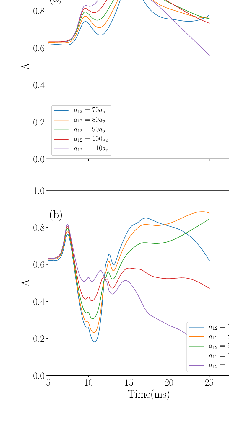
In addition, we observe the peak Rabi frequency plays an important role in determining the miscibility between the two components during light matter interaction. This is in contrast to the case when the light field is absent, that is, miscibility of two condensates is determined by the intra and intercomponent interactions. To illustrate this, we have considered Rabi frequencies, and , for which both the condensates and have finite number of atoms and , even after the light matter interaction. For these two cases we show the variation of the miscibility parameter with time in Fig 6. Note that just after the initiation of transfer process, condensate grows within the condensate , resulting in gradual increase of . When sufficient number of atoms have been transferred to condensate and both the pulses have significant temporal overlap, mutual repulsion between the condensates and the optical dipole potential tend to push the two condensates away from each other. This results in decrease of . Again, the overlap between the condensates and hence increases as pulses gradually die down. It is important to notice that during the light matter interaction we obtain larger values of for larger values of . This indicates, the stronger is the intercomponent repulsion between the two condensates, the larger is the overlap between them. This should be contrasted with the case when light matter interaction is absent, in which, larger intercomponent repulsion separates the condensates spatially. After the light matter interaction, that is, when the optical dipole potentials disappear, the miscibility between the condensates is determined by intra and intercomponent interactions.

V Conclusions
In conclusion, we have shown that how two photon Raman transition can be used to generate a rotating BEC with vorticity of either sign, by transferring atoms from another condensate. In this transition, atoms gain angular momentum from the LG laser pulse before being transferred to rotating condensate.
Density profiles of the condensates during the light-matter interaction depend on sign of the vorticity of the rotating condensate. The growth of a condensate with unit vorticity is started from the central region of the trap, but a condensate with unit vorticity starts to grow from the peripheral region of the trap. The number of transferred atoms can be monitored by tuning intercomponent interaction, if the peak Rabi frequency of light-matter interaction is low and in particular, large intercomponent interaction subdues this transfer process. Finally, another major finding from our investigation is that intercomponent interaction kind of plays opposite role in the process of phase separation during the Raman transition process, in contrast to literature Trippenbach et al. 2000 when such dynamical perturbation is absent.
Finally we point out that the storage of a photon pair entangled in OAM space through Raman transition in cold atomic ensemble has served as sandbox to study information processing Ding et al. 2015. Besides, because atoms can have higher spin manifolds than light, the extension of our work to the spinor BEC would be an important study. Various topological properties can be developed in the ground state depending on Rabi frequency and atom-atom interaction strength, for example, a Mermin-Ho vortex or a meron pair phase Hu et al. 2015, and might lead to the exhibition of non-Abelian braiding statistics Semenoff and Zhou 2007 which is particularly interesting for topological quantum computing protocols Nayak et al. 2008. We expect our study will shed light for further research in this direction.
Acknowledgements.
K.M. is thankful to Subrata Das from Indian Institute of Technology Kharagpur for technical assistance. K.M. is also grateful to Physical Research Laboratory, Ahmedabad for the hospitality during the initial stages of this work. S.B. and D.A. gratefully thank Arko Roy and Pekko Kuopanportti for insightful discussions.*
Appendix A Hamiltonian And Derivation of equation of motions
Let and be the creation and annihilation operators respectively for atoms at state . The Hamiltonian for interacting boson alkali atoms in a trap potential, with respect to a frame rotating at the frequency of applied laser fields in the rotating wave approximation. can be written as
we have following commutation relations for the bosonic operators:
| (9) | ||||
Now Heisenberg equation of motion gives
| (10) |
| (11) |
| (12) |
Using bosonic commutation relation and Heisenberg equation of motion we get
| (13) | ||||
| (14) | ||||
| (15) | ||||
Eliminating of the field operator adiabatically,
| (16) |
| (17) |
Putting (17) into (13) and (14) we get,
| (18) | ||||
and
| (19) | ||||
Where and , Rabi frequencies of the transitions and , are given by and with and being the corresponding transition dipole moments. we consider . AT , in limit of low energy wave scattering, and neglecting Quantum fluctuation, the field operator can be replaced by a complex valued wavefunction . (11) and (12) become
| (20) | ||||
and
| (21) | ||||
| (22) |
and
| (23) |
Here the BEC is considered to be confined at plane and .
References
- D.S (1997) R. D.S, Phys. Rev. Lett. 79, 2164 (1997).
- Mueller et al. (1998) E. Mueller, P. M. Goldbart, and L.-G. Y., Phys. Rev. A. 57, R1505(R) (1998).
- Onofrio et al. (2000) R. Onofrio, C. Raman, J. Abo-Shaeer, A. Chikkatur, and W. Ketterle, Phys. Rev. Lett. 85, 2228 (2000).
- Kobayashi and Tsubota (2007) M. Kobayashi and M. Tsubota, Phys. Rev. A 76, 045603 (2007).
- White et al. (2011) A. C. White, N. P. Proukakis, A. J. Youd, D. H. Wacks, A. W. Baggaley, and C. F. Barenghi, Journal of Physics: Conference Series 318, 062003 (2011).
- Neely et al. (2013) T. W. Neely, A. S. Bradley, E. C. Samson, S. J. Rooney, E. M. Wright, K. J. H. Law, R. Carretero-González, P. G. Kevrekidis, M. J. Davis, and B. P. Anderson, Phys. Rev. Lett. 111, 235301 (2013).
- Barenghi et al. (2014) C. F. Barenghi, L. Skrbek, and K. R. Sreenivasan, 111, 4647 (2014).
- White et al. (2014) A. C. White, B. P. Anderson, and V. S. Bagnato, 111, 4719 (2014).
- Kwon et al. (2014) W. J. Kwon, G. Moon, J.-y. Choi, S. W. Seo, and Y.-i. Shin, Phys. Rev. A 90, 063627 (2014).
- Seo et al. (2017) S. W. Seo, B. Ko, J. H. Kim, and Y. Shin, Scientific Reports 7, 4587 (2017).
- Fedichev and Shlyapnikov (1999) P. O. Fedichev and G. V. Shlyapnikov, Phys. Rev. A 60, R1779 (1999).
- Fetter and Svidzinsky (2001) A. L. Fetter and A. A. Svidzinsky, Journal of Physics: Condensed Matter 13, R135 (2001).
- Koens and Martin (2012) L. Koens and A. M. Martin, Phys. Rev. A 86, 013605 (2012).
- Kevrekidis et al. (2017) P. G. Kevrekidis, W. Wang, R. Carretero-González, D. J. Frantzeskakis, and S. Xie, Phys. Rev. A 96, 043612 (2017).
- Bandyopadhyay et al. (2017) S. Bandyopadhyay, A. Roy, and D. Angom, Phys. Rev. A 96, 043603 (2017).
- Isoshima and Machida (1999) T. Isoshima and K. Machida, Phys. Rev. A 59, 2203 (1999).
- Virtanen and Salomaa (2002) S. M. M. Virtanen and M. M. Salomaa, Journal of Physics B: Atomic, Molecular and Optical Physics 35, 3967 (2002).
- García-Ripoll and Pérez-García (2000) J. J. García-Ripoll and V. M. Pérez-García, Phys. Rev. Lett. 84, 4264 (2000).
- Coddington et al. (2004) I. Coddington, P. C. Haljan, P. Engels, V. Schweikhard, S. Tung, and E. A. Cornell, Phys. Rev. A 70, 063607 (2004).
- Shin et al. (2004) Y. Shin, M. Saba, M. Vengalattore, T. A. Pasquini, C. Sanner, A. E. Leanhardt, M. Prentiss, D. E. Pritchard, and W. Ketterle, Phys. Rev. Lett. 93, 160406 (2004).
- Isoshima et al. (2007) T. Isoshima, M. Okano, H. Yasuda, K. Kasa, J. A. M. Huhtamäki, M. Kumakura, and Y. Takahashi, Phys. Rev. Lett. 99, 200403 (2007).
- Kuopanportti et al. (2010) P. Kuopanportti, E. Lundh, J. A. M. Huhtamäki, V. Pietilä, and M. Möttönen, Phys. Rev. A 81, 023603 (2010).
- Kuopanportti and Möttönen (2010) P. Kuopanportti and M. Möttönen, Phys. Rev. A 81, 033627 (2010).
- Dodd et al. (1997) R. J. Dodd, K. Burnett, M. Edwards, and C. W. Clark, Phys. Rev. A 56, 587 (1997).
- Choi et al. (2003) S. Choi, L. O. Baksmaty, S. J. Woo, and N. P. Bigelow, Phys. Rev. A 68, 031605 (2003).
- Skryabin (2000) D. V. Skryabin, Phys. Rev. A 63, 013602 (2000).
- Middelkamp et al. (2010) S. Middelkamp, P. G. Kevrekidis, D. J. Frantzeskakis, R. Carretero-González, and P. Schmelcher, Phys. Rev. A 82, 013646 (2010).
- Kuopanportti et al. (2018) P. Kuopanportti, S. Bandyopadhyay, A. Roy, and D. Angom, arXiv:1808.08223 (2018).
- Mateo and Delgado (2006) A. M. n. Mateo and V. Delgado, Phys. Rev. Lett. 97, 180409 (2006).
- Neely et al. (2010) T. W. Neely, E. C. Samson, A. S. Bradley, M. J. Davis, and B. P. Anderson, Phys. Rev. Lett. 104, 160401 (2010).
- Bolda and Walls (1998) E. L. Bolda and D. F. Walls, Phys. Rev. Lett. 81, 5477 (1998).
- Chevy et al. (2001) F. Chevy, K. W. Madison, V. Bretin, and J. Dalibard, Phys. Rev. A 64, 031601 (2001).
- Freilich et al. (2010) D. V. Freilich, D. M. Bianchi, A. M. Kaufman, T. K. Langin, and D. S. Hall, Science 329, 1182 (2010).
- Navarro et al. (2013) R. Navarro, R. Carretero-González, P. J. Torres, P. G. Kevrekidis, D. J. Frantzeskakis, M. W. Ray, E. Altuntaş, and D. S. Hall, Phys. Rev. Lett. 110, 225301 (2013).
- Wilson et al. (2015) K. E. Wilson, Z. L. Newman, J. D. Lowney, and B. P. Anderson, Phys. Rev. A 91, 023621 (2015).
- Marzlin et al. (1997) K.-P. Marzlin, W. Zhang, and E. M. Wright, Phys. Rev. Lett. 79, 4728 (1997).
- Dum et al. (1998) R. Dum, J. I. Cirac, M. Lewenstein, and P. Zoller, Phys. Rev. Lett. 80, 2972 (1998).
- Jackson et al. (1998) B. Jackson, J. F. McCann, and C. S. Adams, Phys. Rev. Lett. 80, 3903 (1998).
- Dobrek et al. (1999) L. Dobrek, M. Gajda, M. Lewenstein, K. Sengstock, G. Birkl, and W. Ertmer, Phys. Rev. A 60, R3381 (1999).
- Petrosyan and You (1999) K. G. Petrosyan and L. You, Phys. Rev. A 59, 639 (1999).
- Ruostekoski (2000) J. Ruostekoski, Phys. Rev. A 61, 041603 (2000).
- Damski et al. (2002) B. Damski, K. Sacha, and J. Zakrzewski, Journal of Physics B: Atomic, Molecular and Optical Physics 35, 4051 (2002).
- Shibayama et al. (2011) H. Shibayama, Y. Yasaku, and T. Kuwamoto, Journal of Physics B: Atomic, Molecular and Optical Physics 44, 075302 (2011).
- Matthews et al. (1999) M. R. Matthews, B. P. Anderson, P. C. Haljan, D. S. Hall, C. E. Wieman, and E. A. Cornell, Phys. Rev. Lett. 83, 2498 (1999).
- Madison et al. (2000) K. W. Madison, F. Chevy, W. Wohlleben, and J. Dalibard, Phys. Rev. Lett. 84, 806 (2000).
- Raman et al. (2001) C. Raman, J. R. Abo-Shaeer, J. M. Vogels, K. Xu, and W. Ketterle, Phys. Rev. Lett. 87, 210402 (2001).
- Henn et al. (2009) E. A. L. Henn, J. A. Seman, G. Roati, K. M. F. Magalhães, and V. S. Bagnato, Journal of Low Temperature Physics 158, 435 (2009).
- Raman et al. (1999) C. Raman, M. Köhl, R. Onofrio, D. S. Durfee, C. E. Kuklewicz, Z. Hadzibabic, and W. Ketterle, Phys. Rev. Lett. 83, 2502 (1999).
- Burger et al. (1999) S. Burger, K. Bongs, S. Dettmer, W. Ertmer, K. Sengstock, A. Sanpera, G. V. Shlyapnikov, and M. Lewenstein, Phys. Rev. Lett. 83, 5198 (1999).
- Caradoc-Davies et al. (1999) B. M. Caradoc-Davies, R. J. Ballagh, and K. Burnett, Phys. Rev. Lett. 83, 895 (1999).
- Leanhardt et al. (2002) A. E. Leanhardt, A. Görlitz, A. P. Chikkatur, D. Kielpinski, Y. Shin, D. E. Pritchard, and W. Ketterle, Phys. Rev. Lett. 89, 190403 (2002).
- Möttönen et al. (2007) M. Möttönen, V. Pietilä, and S. M. M. Virtanen, Phys. Rev. Lett. 99, 250406 (2007).
- Xu et al. (2008) Z. F. Xu, P. Zhang, C. Raman, and L. You, Phys. Rev. A 78, 043606 (2008).
- Allen et al. (1992) L. Allen, M. W. Beijersbergen, R. J. C. Spreeuw, and J. P. Woerdman, Phys. Rev. A 45, 8185 (1992).
- Tabosa and Petrov (1999) J. W. R. Tabosa and D. V. Petrov, Phys. Rev. Lett. 83, 4967 (1999).
- He et al. (1995) H. He, M. E. J. Friese, N. R. Heckenberg, and H. Rubinsztein-Dunlop, Phys. Rev. Lett. 75, 826 (1995).
- Kanamoto et al. (2007) R. Kanamoto, E. M. Wright, and P. Meystre, Phys. Rev. A 75, 063623 (2007).
- DeMarco and Pu (2015) M. DeMarco and H. Pu, Phys. Rev. A 91, 033630 (2015).
- Chen et al. (2016) L. Chen, H. Pu, and Y. Zhang, Phys. Rev. A 93, 013629 (2016).
- Nandi et al. (2004) G. Nandi, R. Walser, and W. P. Schleich, Phys. Rev. A 69, 063606 (2004).
- Simula et al. (2008) T. P. Simula, N. Nygaard, S. X. Hu, L. A. Collins, B. I. Schneider, and K. Mølmer, Phys. Rev. A 77, 015401 (2008).
- Jain and Boninsegni (2011) P. Jain and M. Boninsegni, Phys. Rev. A 83, 023602 (2011).
- Roy and Angom (2015) A. Roy and D. Angom, Phys. Rev. A 92, 011601 (2015).
- Peters et al. (2005) T. Peters, L. P. Yatsenko, and T. Halfmann, Phys. Rev. Lett. 95, 103601 (2005).
- Goto and Ichimura (2006) H. Goto and K. Ichimura, Phys. Rev. A 74, 053410 (2006).
- Volz et al. (2006) J. Volz, M. Weber, D. Schlenk, W. Rosenfeld, J. Vrana, K. Saucke, C. Kurtsiefer, and H. Weinfurter, Phys. Rev. Lett. 96, 030404 (2006).
- Longhi et al. (2007) S. Longhi, G. Della Valle, M. Ornigotti, and P. Laporta, Phys. Rev. B 76, 201101 (2007).
- Liu et al. (2016) T. Liu, A. S. Solntsev, A. Boes, T. Nguyen, C. Will, A. Mitchell, D. N. Neshev, and A. A. Sukhorukov, Opt. Lett. 41, 5278 (2016).
- Chung et al. (2015) H. P. Chung, K. H. Huang, S. L. Yang, W. K. Chang, C. W. Wu, F. Setzpfandt, T. Pertsch, D. N. Neshev, and Y. H. Chen, Opt. Express 23, 30641 (2015).
- Panda et al. (2016) C. D. Panda, B. R. O’Leary, A. D. West, J. Baron, P. W. Hess, C. Hoffman, E. Kirilov, C. B. Overstreet, E. P. West, D. DeMille, J. M. Doyle, and G. Gabrielse, Phys. Rev. A 93, 052110 (2016).
- Unanyan et al. (1998) R. Unanyan, M. Fleischhauer, B. Shore, and K. Bergmann, Optics Communications 155, 144 (1998).
- Unanyan et al. (1999) R. G. Unanyan, B. W. Shore, and K. Bergmann, Phys. Rev. A 59, 2910 (1999).
- Kis et al. (2004) Z. Kis, A. Karpati, B. W. Shore, and N. V. Vitanov, Phys. Rev. A 70, 053405 (2004).
- Unanyan et al. (2004) R. G. Unanyan, M. E. Pietrzyk, B. W. Shore, and K. Bergmann, Phys. Rev. A 70, 053404 (2004).
- Wright et al. (2008) K. Wright, L. Leslie, and N. Bigelow, Phys. Rev. A 77, 041601(R) (2008).
- Mondal et al. (2014) P. Mondal, D. Bimalendu, and M. S., Phys. Rev. A 89, 063418 (2014).
- Kamsap et al. (2013) M. R. Kamsap, T. B. Ekogo, J. Pedregosa-Gutierrez, G. Hagel, M. Houssin, O. Morizot, M. Knoop, and C. Champenois, Journal of Physics B: Atomic, Molecular and Optical Physics 46, 145502 (2013).
- Wright et al. (2000) E. Wright, J. Arlt, and D. K., Phys. Rev. A 63, 013608 (2000).
- Timmermans (1998) E. Timmermans, Phys. Rev. Lett. 81, 5718 (1998).
- Wen et al. (2012) L. Wen, W. M. Liu, Y. Cai, J. M. Zhang, and J. Hu, Phys. Rev. A 85, 043602 (2012).
- Bergmann et al. (1998) K. Bergmann, H. Theuer, and S. B.W., Rev. Mod. Phys. 70, 1003 (1998).
- Grigoryan and T. (2001) G. G. Grigoryan and P. Y. T., Phys. Rev. A. 64, 013816 (2001).
- Muruganandam and Adhikari (2009) P. Muruganandam and S. Adhikari, Comput. Phys. Commun. 180, 1888 (2009).
- Vudragović et al. (2012) D. Vudragović, I. Vidanović, A. Balaž, P. Muruganandam, and S. K. Adhikari, Comput. Phys. Commun. 183, 2021 (2012).
- Egorov et al. (2013) M. Egorov, B. Opanchuk, P. Drummond, H. B.V, and S. A.I., Phys. Rev. A. 87, 053614 (2013).
- Mertes et al. (2007) K. Mertes, J. Merrill, R. Carretero-Gonzalez, D. Frantzeskakis, P. Kevrekidis, and D. Hall, Phys. Rev. Lett. 99, 190402 (2007).
- Tojo et al. (2010) S. Tojo, Y. Taguchi, Y. Masuyama, T. Hayashi, H. Saito, and T. Hirano, Phys. Rev. A 82, 033609 (2010).
- Trippenbach et al. (2000) M. Trippenbach, K. Góral, K. Rzazewski, B. Malomed, and Y. B. Band, Journal of Physics B: Atomic, Molecular and Optical Physics 33, 4017 (2000).
- Ding et al. (2015) D.-S. Ding, W. Zhang, Z.-Y. Zhou, S. Shi, G.-Y. Xiang, X.-S. Wang, Y.-K. Jiang, B.-S. Shi, and G.-C. Guo, Phys. Rev. Lett. 114, 050502 (2015).
- Hu et al. (2015) Y.-X. Hu, C. Miniatura, and B. Grémaud, Phys. Rev. A 92, 033615 (2015).
- Semenoff and Zhou (2007) G. W. Semenoff and F. Zhou, Phys. Rev. Lett. 98, 100401 (2007).
- Nayak et al. (2008) C. Nayak, S. H. Simon, A. Stern, M. Freedman, and S. Das Sarma, Rev. Mod. Phys. 80, 1083 (2008).