跳到论文正文
W Papers独立论文阅读器 arXiv:1906.01774 论文正文 计算阅读时间 · 0%
引用这篇论文根据当前论文元数据生成,正式投稿前建议核对。


License: arXiv.org perpetual non-exclusive license
arXiv:1906.01774v2 [cs.IT] 17 Sep 2019

RIP-based performance guarantee for low-tubal-rank tensor recoveryJournal: Journal of Templates

Feng Zhang Email: zhangf@email.swu.edu.cn Address: School of Mathematics and Statistics, Southwest University, Chongqing, 400715, China    Wendong Wang Email: d.sylan@foxmail.com Address: School of Mathematics and Statistics, Southwest University, Chongqing, 400715, China    Jianwen Huang Email: hjw1303987297@126.com Address: School of Mathematics and Statistics, Southwest University, Chongqing, 400715, China    Yao Wang Email: yao.s.wang@gmail.com Address: School of Mathematics and Statistics, Xi’an Jiaotong University, Xi’an, 710049, China    Jianjun Wang Email: wjj@swu.edu.cn Corresponding author: Corresponding author Address: College of Artificial Intelligence, Southwest University, Chongqing, 400715, China
Abstract

The essential task of tensor data analysis focuses on the tensor decomposition and the corresponding notion of rank. In this paper, by introducing the notion of tensor Singular Value Decomposition (t-SVD), we establish a Regularized Tensor Nuclear Norm Minimization (RTNNM) model for low-tubal-rank tensor recovery. As we know that many variants of the Restricted Isometry Property (RIP) have proven to be crucial analysis tools for sparse recovery. In the t-SVD framework, we initiatively define a novel tensor Restricted Isometry Property (t-RIP). Furthermore, we show that any third-order tensor 𝓧\boldsymbol{\mathcal{X}} can stably be recovered from few linear noise measurements under some certain t-RIP conditions via the RTNNM model. We note that, as far as the authors are aware, such kind of result has not previously been reported in the literature.

Keywords: 
Low-rank tensor recovery, tensor Singular Value Decomposition, tensor Restricted Isometry Property, regularized
2010 MSC
90C25, 65J22, 53A45, 15A69

1 Introduction

Utilizing the tensor model, possessed of the ability to make full use of multi-linear structure, instead of the traditional matrix-based model to analyze multi-dimensional data (tensor data) has widely attracted attention. Indeed, in the real world, the carriers of information processing are more commonly tensor data containing more complex information and structures, such as video, hyperspectral images and communication networks stream data, etc. Low-Rank Tensor Recovery (LRTR) as a representative problem is not only a mathematical natural generalization of the Compressed Sensing (CS) and Low-Rank Matrix Recovery (LRMR) problem, but also there exists lots of reconstruction applications of data that have intrinsically many dimensions in the context of LRTR including signal processing [1, 2], machine learning [3, 4], data mining [5, 6], and many others [7, 8, 9, 10, 11].

The purpose of LRTR is to reconstruct a low-rank tensor 𝓧∈ℝn1×n2×n3\boldsymbol{\mathcal{X}}\in\mathbb{R}^{n_{1}\times n_{2}\times n_{3}} (this article considers only the third-order tensor without loss of generality) from linear noise measurements 𝒚=𝕸⁡(𝓧)+𝒘\boldsymbol{y}=\boldsymbol{\mathfrak{M}}(\boldsymbol{\mathcal{X}})+\boldsymbol{w}, where 𝕸:ℝn1×n2×n3→ℝm\boldsymbol{\mathfrak{M}}:\mathbb{R}^{n_{1}\times n_{2}\times n_{3}}\rightarrow\mathbb{R}^{m} (m≪n1​n2​n3)(m\ll n_{1}n_{2}n_{3}) is a random map with i.i.d. Gaussian entries and 𝒘∈ℝm\boldsymbol{w}\in\mathbb{R}^{m} is a vector of measurement errors. To be specific, we consider addressing the following rank minimization problem

min⁡rank𝓧∈ℝn1×n2×n3⁡(𝓧),s.t.‖𝒚−𝕸⁡(𝓧)‖2≤ϵ,\min\limits_{{\boldsymbol{\mathcal{X}}}\in\mathbb{R}^{n_{1}\times n_{2}\times n_{3}}}~\mathop{\rm rank}(\boldsymbol{\mathcal{X}}),~~s.t.~~\|\boldsymbol{y}-\boldsymbol{\mathfrak{M}}(\boldsymbol{\mathcal{X}})\|_{2}\leq\epsilon, (1)

where ϵ\epsilon is a positive constant. However, there exist two tough problems in dealing with model (1). First, the rank minimization problem (1) is NP-hard and non-convex. Second, how should the rank of a tensor be defined? Unlike the unique definition of matrix rank, there exist different notions of tensor rank induced by different tensor decompositions. For example, the CANDECOMP/PARAFAC (CP) rank is defined as the minimum number of rank-1 tensors required to achieve the CP decomposition [12]; The Tucker rank induced by the Tucker decomposition [13] is defined as a vector whose ii-th element is the rank of the mode-ii unfolding matrix of a tensor. However, computing the CP rank of a tensor is already NP-hard in general and its convex relaxation is also intractable. Although the Tucker rank is tractable, its convex surrogate, Sum of Nuclear Norms (SNN) as [1], is not the tightest convex relaxation, which will lead to that the surrogate model can be substantially suboptimal [14].

Recently, based on the definition of tensor Singular Value Decomposition (t-SVD) [15, 16] that enjoys many similar properties as the matrix case, the tensor tubal rank (see Definition 2.8) is proposed by Kilmer et al. [17]. Along those lines, Lu et al. [7] given a new and rigorous way to define the tensor average rank (see Definition 2.9) and the tensor nuclear norm (see Definition 2.10), and proved that the convex envelop of tensor average rank is tensor nuclear norm within the unit ball of the tensor spectral norm. Furthermore, they pointed out that a tensor always has low average rank if it has low tubal rank. Therefore, a convex tensor nuclear norm minimization (TNNM) model based on the assumption of low tubal rank for tensor recovery has been proposed in [7], which solves

min𝓧∈ℝn1×n2×n3⁡‖𝓧‖∗,s.t.‖𝒚−𝕸⁡(𝓧)‖2≤ϵ,\min\limits_{{\boldsymbol{\mathcal{X}}}\in\mathbb{R}^{n_{1}\times n_{2}\times n_{3}}}~\|\boldsymbol{\mathcal{X}}\|_{*},~~s.t.~~\|\boldsymbol{y}-\boldsymbol{\mathfrak{M}}(\boldsymbol{\mathcal{X}})\|_{2}\leq\epsilon, (2)

where tensor nuclear norm ∥⋅∥∗\|\cdot\|_{*} is as the convex surrogate of tensor average rank.

In order to facilitate the design of algorithms and the needs of practical applications, instead of considering the constrained-TNNM (2), in this paper, we present a theoretical analysis for Regularized Tensor Nuclear Norm Minimization (RTNNM) model, which takes the form

min𝓧∈ℝn1×n2×n3⁡‖𝓧‖∗+12​λ​‖𝒚−𝕸⁡(𝓧)‖22,\min\limits_{{\boldsymbol{\mathcal{X}}}\in\mathbb{R}^{n_{1}\times n_{2}\times n_{3}}}~\|\boldsymbol{\mathcal{X}}\|_{*}+\frac{1}{2\lambda}\|\boldsymbol{y}-\boldsymbol{\mathfrak{M}}(\boldsymbol{\mathcal{X}})\|_{2}^{2}, (3)

where λ\lambda is a positive parameter. According to [18], there exists a λ>0\lambda>0 such that the solution to the regularization problem (3) also solves the constrained problem (2) for any ϵ>0\epsilon>0, and vice versa. However, model (3) is more commonly used than model (2) when the noise level is not given or cannot be accurately estimated. There are many examples of solving RTNNM problem (3) based on the tensor nuclear norm heuristic. For instance, the low-tubal-rank tensor completion problem [10] can be thought of as partial observations under the identity transformation and solved as a special case of the RTNNM problem (3) in an alternating direction method of multipliers (ADMM) [19] framework. While the application and algorithm research of (3) is already well-developed, only a few contributions on the theoretical results with regard to performance guarantee for low-tubal-rank tensor recovery are available so far. The Restricted Isometry Property (RIP) introduced by Candès et al. [20] and Recht et al. [21] is one of the most widely used frameworks in CS and LRMR. In this paper, we generalize the RIP tool to tensor case based on t-SVD and establish the guaranteed conditions for low-tubal-rank tensor recovery.

As we know, different tensor decompositions induce different notions of tensor rank, which will lead to different notions of the tensor RIP. For example, in 2013, Shi et al. [11] defined the first tensor RIP based on Tucker decomposition and showed that a tensor 𝓧∈ℝn1×n2×n3\boldsymbol{\mathcal{X}}\in\mathbb{R}^{n_{1}\times n_{2}\times n_{3}} with Tucker rank-(r1,r2,r3)(r_{1},r_{2},r_{3}) can be exactly reconstructed in the noiseless case if the linear map 𝕸\boldsymbol{\mathfrak{M}} satisfies the tensor RIP with the constant δΛ<0.4931\delta_{\Lambda}<0.4931 for Λ∈{(2​r1,n2,n3),(n1,2​r2,n3),(n1,n2,2​r3)}\Lambda\in\left\{(2r_{1},n_{2},n_{3}),(n_{1},2r_{2},n_{3}),(n_{1},n_{2},2r_{3})\right\}; In 2017, based on three variants of Tucker decomposition, i.e., the Higher Order Singular Value Decomposition (HOSVD), the Tensor Train format (TT), and the general Hierarchical Tucker decomposition (HT), Rauhut et al. [8] also induced three notions of the tensor RIP. These tensor RIP definitions are difficult to implement due to relying on a rank tuple that differs greatly from the known matrix rank definition, which would result in some existing analysis tools and techniques not being available for tensor cases. In contrast, the tensor tubal rank induced by the t-SVD is consistent with the matrix rank in terms of form and properties. So, we initiatively define a novel tensor Restricted Isometry Property as follows:

Definition 1.1.

(t-RIP) A linear map 𝕸:ℝn1×n2×n3→ℝm\boldsymbol{\mathfrak{M}}:\mathbb{R}^{n_{1}\times n_{2}\times n_{3}}\rightarrow\mathbb{R}^{m}, is said to satisfy the t-RIP of order rr with tensor Restricted Isometry Constant (t-RIC) δr𝕸\delta_{r}^{\boldsymbol{\mathfrak{M}}} if δr𝕸\delta_{r}^{\boldsymbol{\mathfrak{M}}} is the smallest value δ𝕸∈(0,1)\delta^{\boldsymbol{\mathfrak{M}}}\in(0,1) such that

(1−δ𝕸)​‖𝓧‖F2≤‖𝕸⁡(𝓧)‖22≤(1+δ𝕸)​‖𝓧‖F2(1-\delta^{\boldsymbol{\mathfrak{M}}})\|\boldsymbol{\mathcal{X}}\|_{F}^{2}\leq\|\boldsymbol{\mathfrak{M}}(\boldsymbol{\mathcal{X}})\|_{2}^{2}\leq(1+\delta^{\boldsymbol{\mathfrak{M}}})\|\boldsymbol{\mathcal{X}}\|_{F}^{2} (4)

holds for all tensors 𝓧∈ℝn1×n2×n3\boldsymbol{\mathcal{X}}\in\mathbb{R}^{n_{1}\times n_{2}\times n_{3}} whose tubal rank is at most rr.

Note that the above definition is the natural generalization of the RIP from vectors and matrices to tensors. However, similar to LRMR and different from CS, One cannot view our t-RIC for low-tubal-rank tensor as the condition that all sub-tensors of 𝕸\boldsymbol{\mathfrak{M}} of a given size are well conditioned. Surprisingly, we are still able to derive analogous recovery results for the LRTR problem if the t-RIC of 𝕸\boldsymbol{\mathfrak{M}} satisfies certain conditions. As pointed out by an anonymous reviewer, we should explain why we assume that 𝕸\boldsymbol{\mathfrak{M}} contains i.i.d. Gaussian entries. That’s because in our previous work [22] we have proved that the random Gaussian measurement operator 𝕸\boldsymbol{\mathfrak{M}} satisfies a t-RIP at tubal rank rr with high probability.

Next, let us review some existing theoretical results that will provide us with some inspiration. For constrained CS and LRMR, different conditions on the RIC have been introduced and studied in the literature [23, 24, 25], etc. Among these sufficient conditions, especially, Cai and Zhang [26] showed that for any given t≥4/3t\geq 4/3, the RIC δt​r𝑴<t−1t\delta_{tr}^{\boldsymbol{M}}<\sqrt{\frac{t-1}{t}} for the vector case is sharp (the RIC δt​r𝓜<t−1t\delta_{tr}^{\boldsymbol{\mathcal{M}}}<\sqrt{\frac{t-1}{t}} for the matrix case) ensures the exact recovery in the noiseless case and stable recovery in the noisy case for rr-sparse signals (matrices with rank at most rr). In addition, Zhang and Li [27] obtained another part of the sharp condition, that is δt​r𝑴<t4−t​(δt​r𝓜<t4−t)\delta_{tr}^{\boldsymbol{M}}<\frac{t}{4-t}(\delta_{tr}^{\boldsymbol{\mathcal{M}}}<\frac{t}{4-t}) with 0<t<4/30<t<4/3. The results mentioned above are currently the best in the field. In view of unconstrained sparse vector recovery, as far as we know that Zhu [28] first studied this kind of problem in 2008 and he pointed out that rr-sparse signals can be recovered stably if δ4​r𝑴+2​δ5​r𝑴<1\delta_{4r}^{\boldsymbol{M}}+2\delta_{5r}^{\boldsymbol{M}}<1. Next, in 2015, Shen et al. [29] got a sufficient condition δ2​r𝑴<0.2\delta_{2r}^{\boldsymbol{M}}<0.2 under redundant tight frames. Recently, Ge et al. [30] proved that if the noisy vector 𝒘\boldsymbol{w} satisfies the ℓ∞\ell_{\infty} bounded noise constraint (i.e., ‖𝑴∗​𝒘‖∞≤λ/2\|\boldsymbol{M}^{*}\boldsymbol{w}\|_{\infty}\leq\lambda/2) and δt​r𝑴<t−1t+8\delta_{tr}^{\boldsymbol{M}}<\sqrt{\frac{t-1}{t+8}} with t>1t>1, then rr-sparse signals can be stably recovered. For unconstrained LRMR, the sufficient condition δt​r𝓜<(t−1)/t\delta_{tr}^{\boldsymbol{\mathcal{M}}}<\sqrt{(t-1)/t} for t>1t>1 and error upper bound estimation have been derived in our previous work [31].

Equipped with the t-RIP, in this paper, we aim to construct sufficient conditions for stable low-tubal-rank tensor recovery and obtain an upper bound estimate of error via solving (3). The rest of the paper is organized as follows. In Section 2, we introduce some notations and definitions. In Section 3, we give some key lemmas. In Section 4, our main result is presented. In Section 5, some numerical experiments are conducted to support our analysis. The conclusion is addressed in Section 6. Finally, A provides the proof of Lemma 3.2.

2 Notations and Preliminaries

We use lowercase letters for the entries, e.g. xx, boldface letters for vectors, e.g. 𝒙\boldsymbol{x}, capitalized boldface letters for matrices, e.g. 𝑿\boldsymbol{X} and capitalized boldface calligraphic letters for tensors, e.g. 𝓧\boldsymbol{\mathcal{X}}. For a third-order tensor 𝓧\boldsymbol{\mathcal{X}}, 𝓧(i,:,:)\boldsymbol{\mathcal{X}}(i,:,:), 𝓧(:,i,:)\boldsymbol{\mathcal{X}}(:,i,:) and 𝓧(:,:,i)\boldsymbol{\mathcal{X}}(:,:,i) are used to represent the iith horizontal, lateral, and frontal slice. The frontal slice 𝓧(:,:,i)\boldsymbol{\mathcal{X}}(:,:,i) can also be denoted as 𝑿(i)\boldsymbol{X}^{(i)}. The tube is denoted as 𝓧(i,j,:)\boldsymbol{\mathcal{X}}(i,j,:). We denote the Frobenius norm as ‖𝓧‖F=∑i​j​k|xi​j​k|2\|\boldsymbol{\mathcal{X}}\|_{F}=\sqrt{\sum_{ijk}|x_{ijk}|^{2}}. Defining some norms of matrix is also necessary. We denote by ‖𝑿‖F=∑i​j|xi​j|2=∑iσi2​(𝑿)\|\boldsymbol{X}\|_{F}=\sqrt{\sum_{ij}|x_{ij}|^{2}}=\sqrt{\sum_{i}\sigma_{i}^{2}(\boldsymbol{X})} the Frobenius norm of 𝑿\boldsymbol{X} and denote by ‖𝑿‖∗=∑iσi​(𝑿)\|\boldsymbol{X}\|_{*}=\sum_{i}\sigma_{i}(\boldsymbol{X}) the nuclear norm of 𝑿\boldsymbol{X}, where σi​(𝑿)\sigma_{i}(\boldsymbol{X})’s are the singular values of 𝑿\boldsymbol{X} and σ⁡(𝑿)\sigma(\boldsymbol{X}) represents the singular value vector of matrix 𝑿\boldsymbol{X}. Given a positive integer κ\kappa, we denote [κ]={1,2,⋯,κ}[\kappa]=\{1,2,\cdots,\kappa\} and Γc=[κ]∖Γ\Gamma^{c}=[\kappa]\setminus\Gamma for any Γ⊂[κ]\Gamma\subset[\kappa]. The set of indices of the nonzero entries of a vector 𝒗\boldsymbol{v} is called the support of 𝒗\boldsymbol{v} and denoted as supp(𝒗)\mathop{\rm supp}(\boldsymbol{v}). |Γ||\Gamma| is the cardinality for the index set.

For a third-order tensor 𝓧\boldsymbol{\mathcal{X}}, let 𝓧¯\boldsymbol{\bar{\mathcal{X}}} be the discrete Fourier transform (DFT) along the third dimension of 𝓧\boldsymbol{\mathcal{X}}, i.e., 𝓧¯=fft⁡(𝓧,[],3)\boldsymbol{\bar{\mathcal{X}}}=\rm fft(\boldsymbol{\mathcal{X}},[],3). Similarly, 𝓧\boldsymbol{\mathcal{X}} can be calculated from 𝓧¯\boldsymbol{\bar{\mathcal{X}}} by 𝓧=ifft⁡(𝓧¯,[],3)\boldsymbol{\mathcal{X}}=\rm ifft(\boldsymbol{\bar{\mathcal{X}}},[],3). Let 𝑿¯∈ℝn1​n3×n2​n3\boldsymbol{\bar{X}}\in\mathbb{R}^{n_{1}n_{3}\times n_{2}n_{3}} be the block diagonal matrix with each block on diagonal as the frontal slice 𝑿¯(i)\boldsymbol{\bar{X}}^{(i)} of 𝓧¯\boldsymbol{\bar{\mathcal{X}}}, i.e.,

𝑿¯=bdiag(𝓧¯)=(𝑿¯(1)𝑿¯(2)⋱𝑿¯(n3)),\boldsymbol{\bar{X}}=\mathop{\rm bdiag}(\boldsymbol{\bar{\mathcal{X}}})=\left(\begin{array}[]{cccc}\boldsymbol{\bar{X}}^{(1)}&&&\\ &\boldsymbol{\bar{X}}^{(2)}&&\\ &&\ddots&\\ &&&\boldsymbol{\bar{X}}^{(n_{3})}\\ \end{array}\right),

and bcirc(𝓧)∈ℝn1​n3×n2​n3\mathop{\rm bcirc}(\boldsymbol{\mathcal{X}})\in\mathbb{R}^{n_{1}n_{3}\times n_{2}n_{3}} be the block circular matrix, i.e.,

bcirc(𝓧)=(𝑿(1)𝑿(n3)⋯𝑿(2)𝑿(2)𝑿(1)⋯𝑿(3)⋮⋮⋱⋮𝑿(n3)𝑿(n3−1)⋯𝑿(1)).\mathop{\rm bcirc}(\boldsymbol{\mathcal{X}})=\left(\begin{array}[]{cccc}\boldsymbol{X}^{(1)}&\boldsymbol{X}^{(n_{3})}&\cdots&\boldsymbol{X}^{(2)}\\ \boldsymbol{X}^{(2)}&\boldsymbol{X}^{(1)}&\cdots&\boldsymbol{X}^{(3)}\\ \vdots&\vdots&\ddots&\vdots\\ \boldsymbol{X}^{(n_{3})}&\boldsymbol{X}^{(n_{3}-1)}&\cdots&\boldsymbol{X}^{(1)}\\ \end{array}\right).

The unfold\rm unfold operator and its inverse operator fold\rm fold are, respectively, defined as

unfold(𝓧)=(𝑿(1)𝑿(2)⋯𝑿(n3))T,fold(unfold(𝓧))=𝓧.\mathop{\rm unfold}(\boldsymbol{\mathcal{X}})=\left(\begin{array}[]{cccc}\boldsymbol{X}^{(1)}&\boldsymbol{X}^{(2)}&\cdots&\boldsymbol{X}^{(n_{3})}\\ \end{array}\right)^{T},~~\mathop{\rm fold}(\mathop{\rm unfold}(\boldsymbol{\mathcal{X}}))=\boldsymbol{\mathcal{X}}.

Then tensor-tensor product (t-product) between two third-order tensors can be defined as follows.

Definition 2.1.

(t-product [15]) For tensors 𝓐∈ℝn1×n2×n3\boldsymbol{\mathcal{A}}\in\mathbb{R}^{n_{1}\times n_{2}\times n_{3}} and 𝓑∈ℝn2×n4×n3\boldsymbol{\mathcal{B}}\in\mathbb{R}^{n_{2}\times n_{4}\times n_{3}}, the t-product 𝓐∗𝓑\boldsymbol{\mathcal{A}}\ast\boldsymbol{\mathcal{B}} is defined to be a tensor of size n1×n4×n3n_{1}\times n_{4}\times n_{3},

𝓐∗𝓑=fold(bcirc(𝓐)⋅unfold(𝓑)).\boldsymbol{\mathcal{A}}\ast\boldsymbol{\mathcal{B}}=\mathop{\rm fold}(\mathop{\rm bcirc}(\boldsymbol{\mathcal{A}})\cdot\mathop{\rm unfold}(\boldsymbol{\mathcal{B}})).
Definition 2.2.

(Conjugate transpose [15]) The conjugate transpose of a tensor 𝓧\boldsymbol{\mathcal{X}} of size n1×n2×n3n_{1}\times n_{2}\times n_{3} is the n2×n1×n3n_{2}\times n_{1}\times n_{3} tensor 𝓧∗\boldsymbol{\mathcal{X}}^{*} obtained by conjugate transposing each of the frontal slice and then reversing the order of transposed frontal slices 2 through n3n_{3}.

Definition 2.3.

(Identity tensor [15]) The identity tensor 𝓘∈ℝn×n×n3\boldsymbol{\mathcal{I}}\in\mathbb{R}^{n\times n\times n_{3}} is the tensor whose first frontal slice is the n×nn\times n identity matrix, and other frontal slices are all zeros.

Definition 2.4.

(Orthogonal tensor [15]) A tensor 𝓠∈ℝn×n×n3\boldsymbol{\mathcal{Q}}\in\mathbb{R}^{n\times n\times n_{3}} is orthogonal if it satisfies

𝓠∗∗𝓠=𝓠∗𝓠∗=𝓘.\boldsymbol{\mathcal{Q}}^{*}\ast\boldsymbol{\mathcal{Q}}=\boldsymbol{\mathcal{Q}}\ast\boldsymbol{\mathcal{Q}}^{*}=\boldsymbol{\mathcal{I}}.
Definition 2.5.

(F-diagonal tensor [15]) A tensor is called F-diagonal if each of its frontal slices is a diagonal matrix.

Theorem 2.6.

(t-SVD [15]) Let 𝓧∈ℝn1×n2×n3\boldsymbol{\mathcal{X}}\in\mathbb{R}^{n_{1}\times n_{2}\times n_{3}}, the t-SVD factorization of tensor 𝓧\boldsymbol{\mathcal{X}} is

𝓧=𝓤∗𝓢∗𝓥∗,\boldsymbol{\mathcal{X}}=\boldsymbol{\mathcal{U}}\ast\boldsymbol{\mathcal{S}}\ast\boldsymbol{\mathcal{V}}^{*},

where 𝓤∈ℝn1×n1×n3\boldsymbol{\mathcal{U}}\in\mathbb{R}^{n_{1}\times n_{1}\times n_{3}} and 𝓥∈ℝn2×n2×n3\boldsymbol{\mathcal{V}}\in\mathbb{R}^{n_{2}\times n_{2}\times n_{3}} are orthogonal, 𝓢∈ℝn1×n2×n3\boldsymbol{\mathcal{S}}\in\mathbb{R}^{n_{1}\times n_{2}\times n_{3}} is an F-diagonal tensor. Figure 1 illustrates the t-SVD factorization.

Refer to caption
Figure 1: An illustration of the t-SVD of an n1×n1×n3n_{1}\times n_{1}\times n_{3} tensor.
Remark 2.7.

For κ=min⁡(n1,n2)\kappa=\min(n_{1},n_{2}), the t-SVD of 𝓧\boldsymbol{\mathcal{X}} can be written

𝓧=∑i=1κ𝓤𝓧(:,i,:)∗𝓢𝓧(i,i,:)∗𝓥𝓧(:,i,:)∗.\boldsymbol{\mathcal{X}}=\sum\nolimits_{i=1}^{\kappa}\boldsymbol{\mathcal{U}}_{\boldsymbol{\mathcal{X}}}(:,i,:)\ast\boldsymbol{\mathcal{S}}_{\boldsymbol{\mathcal{X}}}(i,i,:)\ast\boldsymbol{\mathcal{V}}_{\boldsymbol{\mathcal{X}}}(:,i,:)^{*}.

The diagonal vector of the first frontal slice of 𝓢𝓧\boldsymbol{\mathcal{S}}_{\boldsymbol{\mathcal{X}}} is denoted as 𝐬𝓧\boldsymbol{s}_{\boldsymbol{\mathcal{X}}}. The best rr-term approximation of 𝓗\boldsymbol{\mathcal{H}} with the tubal rank at most rr is denoted by

𝓧max⁡(r)=argminrankt(𝓧~)≤r∥𝓧−𝓧~∥F=∑i=1r𝓤𝓧(:,i,:)∗𝓢𝓧(i,i,:)∗𝓥𝓧(:,i,:)∗,\boldsymbol{\mathcal{X}}_{\max(r)}=\arg\min_{\mathop{\rm rank}_{t}(\boldsymbol{\tilde{\mathcal{X}}})\leq r}\|\boldsymbol{\mathcal{X}}-\boldsymbol{\tilde{\mathcal{X}}}\|_{F}=\sum\nolimits_{i=1}^{r}\boldsymbol{\mathcal{U}}_{\boldsymbol{\mathcal{X}}}(:,i,:)\ast\boldsymbol{\mathcal{S}}_{\boldsymbol{\mathcal{X}}}(i,i,:)\ast\boldsymbol{\mathcal{V}}_{\boldsymbol{\mathcal{X}}}(:,i,:)^{*},

and 𝓧−max⁡(r)=𝓧−𝓧max⁡(r)\boldsymbol{\mathcal{X}}_{-\max(r)}=\boldsymbol{\mathcal{X}}-\boldsymbol{\mathcal{X}}_{\max(r)}. In addition, for index set Γ\Gamma, we have

𝓧Γ=∑i∈Γ𝓤𝓧(:,i,:)∗𝓢𝓧(i,i,:)∗𝓥𝓧(:,i,:)∗.\boldsymbol{\mathcal{X}}_{\Gamma}=\sum\nolimits_{i\in\Gamma}\boldsymbol{\mathcal{U}}_{\boldsymbol{\mathcal{X}}}(:,i,:)\ast\boldsymbol{\mathcal{S}}_{\boldsymbol{\mathcal{X}}}(i,i,:)\ast\boldsymbol{\mathcal{V}}_{\boldsymbol{\mathcal{X}}}(:,i,:)^{*}.
Definition 2.8.

(Tensor tubal rank [17]) For 𝓧∈ℝn1×n2×n3\boldsymbol{\mathcal{X}}\in\mathbb{R}^{n_{1}\times n_{2}\times n_{3}}, the tensor tubal rank, denoted as rankt(𝓧)\mathop{\rm rank}_{t}(\boldsymbol{\mathcal{X}}), is defined as the number of nonzero singular tubes of 𝓢\boldsymbol{\mathcal{S}}, where 𝓢\boldsymbol{\mathcal{S}} is from the t-SVD of 𝓧=𝓤∗𝓢∗𝓥∗\boldsymbol{\mathcal{X}}=\boldsymbol{\mathcal{U}}\ast\boldsymbol{\mathcal{S}}\ast\boldsymbol{\mathcal{V}}^{*}. We can write

rankt(𝓧)=♯{i:𝓢(i,i,:)≠𝟎}=♯{i:𝓢(i,i,1)≠0}.\mathop{\rm rank}\nolimits_{t}(\boldsymbol{\mathcal{X}})=\sharp\{i:\boldsymbol{\mathcal{S}}(i,i,:)\neq\boldsymbol{0}\}=\sharp\{i:\boldsymbol{\mathcal{S}}(i,i,1)\neq 0\}.
Definition 2.9.

(Tensor average rank [7]) For 𝓧∈ℝn1×n2×n3\boldsymbol{\mathcal{X}}\in\mathbb{R}^{n_{1}\times n_{2}\times n_{3}}, the tensor average rank, denoted as ranka(𝓧)\mathop{\rm rank}_{a}(\boldsymbol{\mathcal{X}}), is defined as

ranka(𝓧)=1n3​rank(bcirc(𝓧))=1n3​rank(bdiag(𝑿¯)).\mathop{\rm rank}\nolimits_{a}(\boldsymbol{\mathcal{X}})=\frac{1}{n_{3}}\mathop{\rm rank}(\mathop{\rm bcirc}(\boldsymbol{\mathcal{X}}))=\frac{1}{n_{3}}\mathop{\rm rank}(\mathop{\rm bdiag}(\boldsymbol{\bar{X}})).
Definition 2.10.

(Tensor nuclear norm [7]) Let 𝓧=𝓤∗𝓢∗𝓥∗\boldsymbol{\mathcal{X}}=\boldsymbol{\mathcal{U}}\ast\boldsymbol{\mathcal{S}}\ast\boldsymbol{\mathcal{V}}^{*} be the t-SVD of 𝓧∈ℝn1×n2×n3\boldsymbol{\mathcal{X}}\in\mathbb{R}^{n_{1}\times n_{2}\times n_{3}}. The tensor nuclear norm of 𝓧\boldsymbol{\mathcal{X}} is defined as ‖𝓧‖∗:=∑i=1r𝓢⁡(i,i,1)\|\boldsymbol{\mathcal{X}}\|_{*}:=\sum_{i=1}^{r}\boldsymbol{\mathcal{S}}(i,i,1), where r=rankt(𝓧)r=\mathop{\rm rank}_{t}(\boldsymbol{\mathcal{X}}).

Proposition 2.11.

For a third-order tensor 𝓧\boldsymbol{\mathcal{X}}, we have the following properties

‖𝓧‖F\displaystyle\|\boldsymbol{\mathcal{X}}\|_{F} =\displaystyle= 1n3​‖𝑿¯‖F,\displaystyle\frac{1}{\sqrt{n_{3}}}\|\boldsymbol{\bar{X}}\|_{F}, (5)
‖𝓧‖∗\displaystyle\|\boldsymbol{\mathcal{X}}\|_{*} =\displaystyle= 1n3​‖𝑿¯‖∗.\displaystyle\frac{1}{n_{3}}\|\boldsymbol{\bar{X}}\|_{*}. (6)
rank(𝑿¯)\displaystyle\mathop{\rm rank}(\boldsymbol{\bar{X}}) ≤\displaystyle\leq n3​rankt(𝓧).\displaystyle n_{3}\mathop{\rm rank}\nolimits_{t}(\boldsymbol{\mathcal{X}}). (7)

3 Some Key Lemmas

We present the following lemmas, which will play a key role in proving our sufficient conditions for low-tubal-rank tensor recovery.

Lemma 3.1.

[26]  For a positive number ϕ\phi and a positive integer ss, define the polytope T⁡(ϕ,s)⊂ℝnT(\phi,s)\subset\mathbb{R}^{n} by

T(ϕ,s)={𝒗∈ℝn:∥𝒗∥∞≤ϕ,∥𝒗∥1≤sϕ}.T(\phi,s)=\{\boldsymbol{v}\in\mathbb{R}^{n}:\|\boldsymbol{v}\|_{\infty}\leq\phi,\|\boldsymbol{v}\|_{1}\leq s\phi\}.

For any 𝐯∈ℝn\boldsymbol{v}\in\mathbb{R}^{n}, define the set of sparse vectors U⁡(ϕ,s,𝐯)⊂ℝnU(\phi,s,\boldsymbol{v})\subset\mathbb{R}^{n} by

U(ϕ,s,𝒗)={𝒖∈ℝn:supp(𝒖)⊆supp(𝒗),∥𝒖∥0≤s,∥𝒖∥1=∥𝒗∥1,∥𝒖∥∞≤ϕ}.U(\phi,s,\boldsymbol{v})=\{\boldsymbol{u}\in\mathbb{R}^{n}:\mathop{\rm supp}(\boldsymbol{u})\subseteq\mathop{\rm supp}(\boldsymbol{v}),\|\boldsymbol{u}\|_{0}\leq s,\|\boldsymbol{u}\|_{1}=\|\boldsymbol{v}\|_{1},\|\boldsymbol{u}\|_{\infty}\leq\phi\}.

Then 𝐯∈T⁡(ϕ,s)\boldsymbol{v}\in T(\phi,s) if and only if 𝐯\boldsymbol{v} is in the convex hull of U⁡(ϕ,s,𝐯)U(\phi,s,\boldsymbol{v}). In particular, any 𝐯∈T⁡(ϕ,s)\boldsymbol{v}\in T(\phi,s) can be expressed as

𝒗=∑i=1Nγi​𝒖i\boldsymbol{v}=\sum_{i=1}^{N}\gamma_{i}\boldsymbol{u}_{i}

where 𝐮i∈U⁡(ϕ,s,𝐯)\boldsymbol{u}_{i}\in U(\phi,s,\boldsymbol{v}) and 0≤γi≤10\leq\gamma_{i}\leq 1, ∑i=1Nγi=1\sum_{i=1}^{N}\gamma_{i}=1.

This elementary technique introduced by T. Cai and A. Zhang [26] shows that any point in a polytope can be represented as a convex combination of sparse vectors and makes the analysis surprisingly simple.

The following lemma shows that a suitable t-RIP condition implies the robust null space property [32] of the linear map 𝕸\boldsymbol{\mathfrak{M}}.

Lemma 3.2.

Let the linear map 𝕸:ℝn1×n2×n3→ℝn\boldsymbol{\mathfrak{M}}:\mathbb{R}^{n_{1}\times n_{2}\times n_{3}}\rightarrow\mathbb{R}^{n} satisfies the t-RIP of order t​r​(t>1)tr(t>1) with t-RIC δt​r𝕸∈(0,1)\delta_{tr}^{\boldsymbol{\mathfrak{M}}}\in(0,1). Then for any tensor 𝓗∈ℝn1×n2×n3\boldsymbol{\mathcal{H}}\in\mathbb{R}^{n_{1}\times n_{2}\times n_{3}} and any subset Γ⊂[κ]\Gamma\subset[\kappa] with |Γ|=r|\Gamma|=r and κ=min⁡(n1,n2)\kappa=\min(n_{1},n_{2}), it holds that

‖𝓗Γ‖F≤η1​‖𝕸⁡(𝓗)‖2+η2r​‖𝓗Γc‖∗,\|\boldsymbol{\mathcal{H}}_{\Gamma}\|_{F}\leq\eta_{1}\|\boldsymbol{\mathfrak{M}}(\boldsymbol{\mathcal{H}})\|_{2}+\frac{\eta_{2}}{\sqrt{r}}\|\boldsymbol{\mathcal{H}}_{\Gamma^{c}}\|_{*}, (8)

where

η1≜2(1−δt​r𝕸)​1+δt​r𝕸,and​η2≜n3​δtr𝕸(1−(δtr𝕸)2)​(t−1).\eta_{1}\triangleq\frac{2}{(1-\delta_{tr}^{\boldsymbol{\mathfrak{M}}})\sqrt{1+\delta_{tr}^{\boldsymbol{\mathfrak{M}}}}},~~\rm and~~\eta_{2}\triangleq\frac{\sqrt{n_{3}}\delta_{tr}^{\boldsymbol{\mathfrak{M}}}}{\sqrt{(1-(\delta_{tr}^{\boldsymbol{\mathfrak{M}}})^{2})(t-1)}}.
Proof.

Please see A. ∎

In order to prove the main result, we still need the following lemma.

Lemma 3.3.

If the noisy measurements 𝐲=𝕸⁡(𝓧)+𝐰\boldsymbol{y}=\boldsymbol{\mathfrak{M}}(\boldsymbol{\mathcal{X}})+\boldsymbol{w} of tensor 𝓧∈ℝn1×n2×n3\boldsymbol{\mathcal{X}}\in\mathbb{R}^{n_{1}\times n_{2}\times n_{3}} are observed with noise level ‖𝐰‖2≤ϵ\|\boldsymbol{w}\|_{2}\leq\epsilon, then for any subset Γ⊂[κ]\Gamma\subset[\kappa] with |Γ|=r|\Gamma|=r and κ=min⁡(n1,n2)\kappa=\min(n_{1},n_{2}), the minimization solution 𝓧^\boldsymbol{\hat{\mathcal{X}}} of (3) satisfies

‖𝕸⁡(𝓗)‖22−2​ϵ​‖𝕸⁡(𝓗)‖2≤2​λ​(‖𝓗Γ‖∗−‖𝓗Γc‖∗+2​‖𝓧Γc‖∗),\|\boldsymbol{\mathfrak{M}}(\boldsymbol{\mathcal{H}})\|_{2}^{2}-2\epsilon\|\boldsymbol{\mathfrak{M}}(\boldsymbol{\mathcal{H}})\|_{2}\leq 2\lambda(\|\boldsymbol{\mathcal{H}}_{\Gamma}\|_{*}-\|\boldsymbol{\mathcal{H}}_{\Gamma^{c}}\|_{*}+2\|\boldsymbol{\mathcal{X}}_{\Gamma^{c}}\|_{*}), (9)

and

‖𝓗Γc‖∗≤‖𝓗Γ‖∗+2​‖𝓧Γc‖∗+ϵλ​‖𝕸⁡(𝓗)‖2,\|\boldsymbol{\mathcal{H}}_{\Gamma^{c}}\|_{*}\leq\|\boldsymbol{\mathcal{H}}_{\Gamma}\|_{*}+2\|\boldsymbol{\mathcal{X}}_{\Gamma^{c}}\|_{*}+\frac{\epsilon}{\lambda}\|\boldsymbol{\mathfrak{M}}(\boldsymbol{\mathcal{H}})\|_{2}, (10)

where 𝓗≜𝓧^−𝓧\boldsymbol{\mathcal{H}}\triangleq\boldsymbol{\hat{\mathcal{X}}}-\boldsymbol{\mathcal{X}}.

Proof.

Since 𝓧^\boldsymbol{\hat{\mathcal{X}}} is the minimizer of (3), we have

‖𝓧^‖∗+12​λ​‖𝒚−𝕸⁡(𝓧^)‖22≤‖𝓧‖∗+12​λ​‖𝒚−𝕸⁡(𝓧)‖22.\|\boldsymbol{\hat{\mathcal{X}}}\|_{*}+\frac{1}{2\lambda}\|\boldsymbol{y}-\boldsymbol{\mathfrak{M}}(\boldsymbol{\hat{\mathcal{X}}})\|_{2}^{2}\leq\|\boldsymbol{\mathcal{X}}\|_{*}+\frac{1}{2\lambda}\|\boldsymbol{y}-\boldsymbol{\mathfrak{M}}(\boldsymbol{\mathcal{X}})\|_{2}^{2}.

Also because 𝓧^=𝓗+𝓧\boldsymbol{\hat{\mathcal{X}}}=\boldsymbol{\mathcal{H}}+\boldsymbol{\mathcal{X}} and 𝒚=𝕸⁡(𝓧)+𝒘\boldsymbol{y}=\boldsymbol{\mathfrak{M}}(\boldsymbol{\mathcal{X}})+\boldsymbol{w}, so the above inequality is equivalent to

‖𝕸⁡(𝓗)‖22−2​⟨𝒘,𝕸⁡(𝓗)⟩≤2​λ​(‖𝓧‖∗−‖𝓧^‖∗).\|\boldsymbol{\mathfrak{M}}(\boldsymbol{\mathcal{H}})\|_{2}^{2}-2\langle\boldsymbol{w},\boldsymbol{\mathfrak{M}}(\boldsymbol{\mathcal{H}})\rangle\leq 2\lambda(\|\boldsymbol{\mathcal{X}}\|_{*}-\|\boldsymbol{\hat{\mathcal{X}}}\|_{*}).

It follows from the Cauchy-Schwartz inequality and assumption ‖𝒘‖2≤ϵ\|\boldsymbol{w}\|_{2}\leq\epsilon that

‖𝕸⁡(𝓗)‖22−2​⟨𝒘,𝕸⁡(𝓗)⟩≥‖𝕸⁡(𝓗)‖22−2​ϵ​‖𝕸⁡(𝓗)‖2.\|\boldsymbol{\mathfrak{M}}(\boldsymbol{\mathcal{H}})\|_{2}^{2}-2\langle\boldsymbol{w},\boldsymbol{\mathfrak{M}}(\boldsymbol{\mathcal{H}})\rangle\geq\|\boldsymbol{\mathfrak{M}}(\boldsymbol{\mathcal{H}})\|_{2}^{2}-2\epsilon\|\boldsymbol{\mathfrak{M}}(\boldsymbol{\mathcal{H}})\|_{2}. (11)

On the other hand, we have

‖𝓧^‖∗−‖𝓧‖∗\displaystyle\|\boldsymbol{\hat{\mathcal{X}}}\|_{*}-\|\boldsymbol{\mathcal{X}}\|_{*} =\displaystyle= ‖(𝓗+𝓧)Γ‖∗+‖(𝓗+𝓧)Γc‖∗−(‖𝓧Γ‖∗+‖𝓧Γc‖∗)\displaystyle\|(\boldsymbol{\mathcal{H}}+\boldsymbol{\mathcal{X}})_{\Gamma}\|_{*}+\|(\boldsymbol{\mathcal{H}}+\boldsymbol{\mathcal{X}})_{\Gamma^{c}}\|_{*}-(\|\boldsymbol{\mathcal{X}}_{\Gamma}\|_{*}+\|\boldsymbol{\mathcal{X}}_{\Gamma^{c}}\|_{*}) (12)
≥\displaystyle\geq (∥𝓧Γ∥∗−∥𝓗Γ∥∗)+(∥𝓗Γc|∗−∥𝓧Γc∥∗)−(∥𝓧Γ∥∗+∥𝓧Γc∥∗)\displaystyle(\|\boldsymbol{\mathcal{X}}_{\Gamma}\|_{*}-\|\boldsymbol{\mathcal{H}}_{\Gamma}\|_{*})+(\|\boldsymbol{\mathcal{H}}_{\Gamma^{c}}|_{*}-\|\boldsymbol{\mathcal{X}}_{\Gamma^{c}}\|_{*})-(\|\boldsymbol{\mathcal{X}}_{\Gamma}\|_{*}+\|\boldsymbol{\mathcal{X}}_{\Gamma^{c}}\|_{*})
≥\displaystyle\geq ‖𝓗Γc|∗−‖​𝓗Γ|∗−2|𝓧Γc|∗.\displaystyle\|\boldsymbol{\mathcal{H}}_{\Gamma^{c}}|_{*}-\|\boldsymbol{\mathcal{H}}_{\Gamma}|_{*}-2\|\boldsymbol{\mathcal{X}}_{\Gamma^{c}}|_{*}.

Combining (11) and (12) and by a simple calculation, we get (9). As to (10), it is obtained by subtracting the term ‖𝕸⁡(𝓗)‖22\|\boldsymbol{\mathfrak{M}}(\boldsymbol{\mathcal{H}})\|_{2}^{2} from the left-hand side of (9). ∎

4 Main Results

With preparations above, now we present our main result.

Theorem 4.1.

For any observed vector 𝐲=𝕸⁡(𝓧)+𝐰\boldsymbol{y}=\boldsymbol{\mathfrak{M}}(\boldsymbol{\mathcal{X}})+\boldsymbol{w} of tensor 𝓧∈ℝn1×n2×n3\boldsymbol{\mathcal{X}}\in\mathbb{R}^{n_{1}\times n_{2}\times n_{3}} corrupted by an unknown noise 𝐰\boldsymbol{w}, with bounded constrain ‖𝐰‖2≤ϵ\|\boldsymbol{w}\|_{2}\leq\epsilon, if 𝕸\boldsymbol{\mathfrak{M}} satisfies t-RIP with

δt​r𝕸<t−1n32+t−1\delta_{tr}^{\boldsymbol{\mathfrak{M}}}<\sqrt{\frac{t-1}{n_{3}^{2}+t-1}} (13)

for certain t>1t>1, then we have

‖𝕸⁡(𝓧^−𝓧)‖2≤C1​‖𝓧−max⁡(r)‖∗+C2,\|\boldsymbol{\mathfrak{M}}(\boldsymbol{\hat{\mathcal{X}}}-\boldsymbol{\mathcal{X}})\|_{2}\leq C_{1}\|\boldsymbol{\mathcal{X}}_{-\max(r)}\|_{*}+C_{2}, (14)

and

‖𝓧^−𝓧‖F≤C3​‖𝓧−max⁡(r)‖∗+C4,\|\boldsymbol{\hat{\mathcal{X}}}-\boldsymbol{\mathcal{X}}\|_{F}\leq C_{3}\|\boldsymbol{\mathcal{X}}_{-\max(r)}\|_{*}+C_{4}, (15)

where 𝓧^\boldsymbol{\hat{\mathcal{X}}} is the solution to (3), and Ci,i=1,2,3,4C_{i},i=1,2,3,4 are denoted as

C1\displaystyle C_{1} =\displaystyle= 2r​η1,C2=2​r​η1​λ+2​ϵ,\displaystyle\frac{2}{\sqrt{r}\eta_{1}},\quad C_{2}=2\sqrt{r}\eta_{1}\lambda+2\epsilon,
C3\displaystyle C_{3} =\displaystyle= 2​r​η1​(2​n3​r+1+η2)​λ+2​(n3​r+η2)​ϵr​η1​(1−η2)​λ,\displaystyle\frac{2\sqrt{r}\eta_{1}(2\sqrt{n_{3}r}+1+\eta_{2})\lambda+2(\sqrt{n_{3}r}+\eta_{2})\epsilon}{r\eta_{1}(1-\eta_{2})\lambda},
C4\displaystyle C_{4} =\displaystyle= (n3​r+1)​η1​λ+(n3​r−n3​η2+n3+1)​ϵ(1−η2)​λ​(2​r​η1​λ+2​ϵ)−1.\displaystyle\frac{(\sqrt{n_{3}r}+1)\eta_{1}\lambda+(\sqrt{n_{3}r}-\sqrt{n_{3}}\eta_{2}+\sqrt{n_{3}}+1)\epsilon}{(1-\eta_{2})\lambda(2\sqrt{r}\eta_{1}\lambda+2\epsilon)^{-1}}.
Proof.

For convenience, let

T=supp(𝒔𝓧max⁡(r))T=\mathop{\rm supp}(\boldsymbol{s}_{\boldsymbol{\mathcal{X}}_{\max(r)}})

be an index set with cardinality |T|≤r|T|\leq r. In addition, if we set 𝓗=𝓧^−𝓧\boldsymbol{\mathcal{H}}=\boldsymbol{\hat{\mathcal{X}}}-\boldsymbol{\mathcal{X}} and rank(bdiag(𝓗¯Γ))=r¯\mathop{\rm rank}(\mathop{\rm bdiag}(\boldsymbol{\bar{\mathcal{H}}}_{\Gamma}))=\bar{r}, then by inequality (8) and (9), we would get

‖𝕸⁡(𝓗)‖22−2​ϵ​‖𝕸⁡(𝓗)‖2\displaystyle\|\boldsymbol{\mathfrak{M}}(\boldsymbol{\mathcal{H}})\|_{2}^{2}-2\epsilon\|\boldsymbol{\mathfrak{M}}(\boldsymbol{\mathcal{H}})\|_{2} ≤\displaystyle\leq 2​λ​(‖𝓗Γ‖∗−‖𝓗Γc‖∗+2​‖𝓧Γc‖∗)\displaystyle 2\lambda(\|\boldsymbol{\mathcal{H}}_{\Gamma}\|_{*}-\|\boldsymbol{\mathcal{H}}_{\Gamma^{c}}\|_{*}+2\|\boldsymbol{\mathcal{X}}_{\Gamma^{c}}\|_{*})
=(a)\displaystyle\stackrel{{\scriptstyle(a)}}{{=}} 2​λ​(1n3​‖bdiag(𝓗¯Γ)‖∗−‖𝓗Γc‖∗+2​‖𝓧Γc‖∗)\displaystyle 2\lambda\left(\frac{1}{n_{3}}\|\mathop{\rm bdiag}(\boldsymbol{\bar{\mathcal{H}}}_{\Gamma})\|_{*}-\|\boldsymbol{\mathcal{H}}_{\Gamma^{c}}\|_{*}+2\|\boldsymbol{\mathcal{X}}_{\Gamma^{c}}\|_{*}\right)
≤\displaystyle\leq 2​λ​(r¯n3​‖bdiag(𝓗¯Γ)‖F−‖𝓗Γc‖∗+2​‖𝓧Γc‖∗)\displaystyle 2\lambda\left(\frac{\sqrt{\bar{r}}}{n_{3}}\|\mathop{\rm bdiag}(\boldsymbol{\bar{\mathcal{H}}}_{\Gamma})\|_{F}-\|\boldsymbol{\mathcal{H}}_{\Gamma^{c}}\|_{*}+2\|\boldsymbol{\mathcal{X}}_{\Gamma^{c}}\|_{*}\right)
≤(b)\displaystyle\stackrel{{\scriptstyle(b)}}{{\leq}} 2​λ​(r​‖𝓗Γ‖F−‖𝓗Γc‖∗+2​‖𝓧Γc‖∗)\displaystyle 2\lambda\left(\sqrt{r}\|\boldsymbol{\mathcal{H}}_{\Gamma}\|_{F}-\|\boldsymbol{\mathcal{H}}_{\Gamma^{c}}\|_{*}+2\|\boldsymbol{\mathcal{X}}_{\Gamma^{c}}\|_{*}\right)
≤\displaystyle\leq 2​r​λ​(η1​‖𝕸⁡(𝓗)‖2+η2r​‖𝓗Γc‖∗)−2​λ​‖𝓗Γc‖∗+4​λ​‖𝓧Γc‖∗\displaystyle 2\sqrt{r}\lambda\left(\eta_{1}\|\boldsymbol{\mathfrak{M}}(\boldsymbol{\mathcal{H}})\|_{2}+\frac{\eta_{2}}{\sqrt{r}}\|\boldsymbol{\mathcal{H}}_{\Gamma^{c}}\|_{*}\right)-2\lambda\|\boldsymbol{\mathcal{H}}_{\Gamma^{c}}\|_{*}+4\lambda\|\boldsymbol{\mathcal{X}}_{\Gamma^{c}}\|_{*}
=\displaystyle= 2​r​η1​λ​‖𝕸⁡(𝓗)‖2−2​(1−η2)​λ​‖𝓗Γc‖∗+4​λ​‖𝓧Γc‖∗,\displaystyle 2\sqrt{r}\eta_{1}\lambda\|\boldsymbol{\mathfrak{M}}(\boldsymbol{\mathcal{H}})\|_{2}-2(1-\eta_{2})\lambda\|\boldsymbol{\mathcal{H}}_{\Gamma^{c}}\|_{*}+4\lambda\|\boldsymbol{\mathcal{X}}_{\Gamma^{c}}\|_{*},

where (a) follows from (6) and (b) is due to (5), (7). The assumption (13) implies that

1−η2=1−n3​δt​r𝕸(1−(δt​r𝕸)2)​(t−1)>1−n3​(t−1)/(n32+t−1)(1−(t−1)/(n32+t−1))​(t−1)=0,1-\eta_{2}=1-\frac{\sqrt{n_{3}}\delta_{tr}^{\boldsymbol{\mathfrak{M}}}}{\sqrt{(1-(\delta_{tr}^{\boldsymbol{\mathfrak{M}}})^{2})(t-1)}}>1-\frac{\sqrt{n_{3}}\sqrt{(t-1)/(n_{3}^{2}+t-1)}}{\sqrt{\left(1-(t-1)/(n_{3}^{2}+t-1)\right)(t-1)}}=0,

and hence

‖𝕸⁡(𝓗)‖22−2​(r​η1​λ+ϵ)​‖𝕸⁡(𝓗)‖2−4​λ​‖𝓧Γc‖∗≤0,\|\boldsymbol{\mathfrak{M}}(\boldsymbol{\mathcal{H}})\|_{2}^{2}-2(\sqrt{r}\eta_{1}\lambda+\epsilon)\|\boldsymbol{\mathfrak{M}}(\boldsymbol{\mathcal{H}})\|_{2}-4\lambda\|\boldsymbol{\mathcal{X}}_{\Gamma^{c}}\|_{*}\leq 0,

which implies that

(‖𝕸⁡(𝓗)‖2−(r​η1​λ+ϵ))2\displaystyle\left(\|\boldsymbol{\mathfrak{M}}(\boldsymbol{\mathcal{H}})\|_{2}-(\sqrt{r}\eta_{1}\lambda+\epsilon)\right)^{2} ≤\displaystyle\leq (r​η1​λ+ϵ)2+4​λ​‖𝓧Γc‖∗\displaystyle(\sqrt{r}\eta_{1}\lambda+\epsilon)^{2}+4\lambda\|\boldsymbol{\mathcal{X}}_{\Gamma^{c}}\|_{*}
≤\displaystyle\leq (r​η1​λ+ϵ+2​λ​‖𝓧Γc‖∗r​η1​λ+ϵ)2\displaystyle\left(\sqrt{r}\eta_{1}\lambda+\epsilon+\frac{2\lambda\|\boldsymbol{\mathcal{X}}_{\Gamma^{c}}\|_{*}}{\sqrt{r}\eta_{1}\lambda+\epsilon}\right)^{2}
≤\displaystyle\leq (r​η1​λ+ϵ+2​‖𝓧Γc‖∗r​η1)2.\displaystyle\left(\sqrt{r}\eta_{1}\lambda+\epsilon+\frac{2\|\boldsymbol{\mathcal{X}}_{\Gamma^{c}}\|_{*}}{\sqrt{r}\eta_{1}}\right)^{2}.

Therefore, we conclude that (14) holds. Plugging (14) into (10), by ‖𝓗Γ‖∗≤r​‖𝓗Γ‖F\|\boldsymbol{\mathcal{H}}_{\Gamma}\|_{*}\leq\sqrt{r}\|\boldsymbol{\mathcal{H}}_{\Gamma}\|_{F}, we get

‖𝓗Γc‖∗\displaystyle\|\boldsymbol{\mathcal{H}}_{\Gamma^{c}}\|_{*} ≤\displaystyle\leq ‖𝓗Γ‖∗+2​‖𝓧Γc‖∗+ϵλ​(2​‖𝓧Γc‖∗r​η1+2​r​η1​λ+2​ϵ)\displaystyle\|\boldsymbol{\mathcal{H}}_{\Gamma}\|_{*}+2\|\boldsymbol{\mathcal{X}}_{\Gamma^{c}}\|_{*}+\frac{\epsilon}{\lambda}\left(\frac{2\|\boldsymbol{\mathcal{X}}_{\Gamma^{c}}\|_{*}}{\sqrt{r}\eta_{1}}+2\sqrt{r}\eta_{1}\lambda+2\epsilon\right) (16)
≤\displaystyle\leq r​‖𝓗Γ‖F+2​(r​η1​λ+ϵ)r​η1​λ​‖𝓧Γc‖∗+ϵλ​(2​r​η1​λ+2​ϵ).\displaystyle\sqrt{r}\|\boldsymbol{\mathcal{H}}_{\Gamma}\|_{F}+\frac{2(\sqrt{r}\eta_{1}\lambda+\epsilon)}{\sqrt{r}\eta_{1}\lambda}\|\boldsymbol{\mathcal{X}}_{\Gamma^{c}}\|_{*}+\frac{\epsilon}{\lambda}(2\sqrt{r}\eta_{1}\lambda+2\epsilon).

Combining (8), (14) and (16) yields

‖𝓗Γ‖F\displaystyle\|\boldsymbol{\mathcal{H}}_{\Gamma}\|_{F} ≤\displaystyle\leq η1​(2​‖𝓧Γc‖∗r​η1+2​r​η1​λ+2​ϵ)\displaystyle\eta_{1}\left(\frac{2\|\boldsymbol{\mathcal{X}}_{\Gamma^{c}}\|_{*}}{\sqrt{r}\eta_{1}}+2\sqrt{r}\eta_{1}\lambda+2\epsilon\right)
+η2r​(r​‖𝓗Γ‖F+2​(r​η1​λ+ϵ)r​η1​λ​‖𝓧Γc‖∗+ϵλ​(2​r​η1​λ+2​ϵ))\displaystyle+\frac{\eta_{2}}{\sqrt{r}}\left(\sqrt{r}\|\boldsymbol{\mathcal{H}}_{\Gamma}\|_{F}+\frac{2(\sqrt{r}\eta_{1}\lambda+\epsilon)}{\sqrt{r}\eta_{1}\lambda}\|\boldsymbol{\mathcal{X}}_{\Gamma^{c}}\|_{*}+\frac{\epsilon}{\lambda}(2\sqrt{r}\eta_{1}\lambda+2\epsilon)\right)
=\displaystyle= η2​‖𝓗Γ‖F+2​r​η1​(1+η2)​λ+2​η2​ϵr​η1​λ​‖𝓧Γc‖∗+(η1+ϵλ)​(2​r​η1​λ+2​ϵ).\displaystyle\eta_{2}\|\boldsymbol{\mathcal{H}}_{\Gamma}\|_{F}+\frac{2\sqrt{r}\eta_{1}(1+\eta_{2})\lambda+2\eta_{2}\epsilon}{r\eta_{1}\lambda}\|\boldsymbol{\mathcal{X}}_{\Gamma^{c}}\|_{*}+(\eta_{1}+\frac{\epsilon}{\lambda})(2\sqrt{r}\eta_{1}\lambda+2\epsilon).

Note that 1−η2>01-\eta_{2}>0, so the above inequality leads to

‖𝓗Γ‖F≤2​r​η1​(1+η2)​λ+2​η2​ϵr​η1​(1−η2)​λ​‖𝓧Γc‖∗+(η1​λ+ϵ)​(2​r​η1​λ+2​ϵ)(1−η2)​λ.\|\boldsymbol{\mathcal{H}}_{\Gamma}\|_{F}\leq\frac{2\sqrt{r}\eta_{1}(1+\eta_{2})\lambda+2\eta_{2}\epsilon}{r\eta_{1}(1-\eta_{2})\lambda}\|\boldsymbol{\mathcal{X}}_{\Gamma^{c}}\|_{*}+\frac{(\eta_{1}\lambda+\epsilon)(2\sqrt{r}\eta_{1}\lambda+2\epsilon)}{(1-\eta_{2})\lambda}. (17)

To prove (15), application of (16) and (17) yields

‖𝓗‖F\displaystyle\|\boldsymbol{\mathcal{H}}\|_{F} ≤\displaystyle\leq ‖𝓗Γ‖F+‖𝓗Γc‖F\displaystyle\|\boldsymbol{\mathcal{H}}_{\Gamma}\|_{F}+\|\boldsymbol{\mathcal{H}}_{\Gamma^{c}}\|_{F}
≤\displaystyle\leq (n3​r+1)​‖𝓗Γ‖F+2​n3​(r​η1​λ+ϵ)r​η1​λ​‖𝓧Γc‖∗+ϵλ​n3​(2​r​η1​λ+2​ϵ)\displaystyle(\sqrt{n_{3}r}+1)\|\boldsymbol{\mathcal{H}}_{\Gamma}\|_{F}+\frac{2\sqrt{n_{3}}(\sqrt{r}\eta_{1}\lambda+\epsilon)}{\sqrt{r}\eta_{1}\lambda}\|\boldsymbol{\mathcal{X}}_{\Gamma^{c}}\|_{*}+\frac{\epsilon}{\lambda}\sqrt{n_{3}}(2\sqrt{r}\eta_{1}\lambda+2\epsilon)
≤\displaystyle\leq (n3​r+1)​(2​r​η1​(1+η2)​λ+2​η2​ϵr​η1​(1−η2)​λ​‖𝓧Γc‖∗+(η1​λ+ϵ)​(2​r​η1​λ+2​ϵ)(1−η2)​λ)\displaystyle(\sqrt{n_{3}r}+1)\left(\frac{2\sqrt{r}\eta_{1}(1+\eta_{2})\lambda+2\eta_{2}\epsilon}{r\eta_{1}(1-\eta_{2})\lambda}\|\boldsymbol{\mathcal{X}}_{\Gamma^{c}}\|_{*}+\frac{(\eta_{1}\lambda+\epsilon)(2\sqrt{r}\eta_{1}\lambda+2\epsilon)}{(1-\eta_{2})\lambda}\right)
+2​n3​(r​η1​λ+ϵ)r​η1​λ​‖𝓧Γc‖∗+ϵλ​n3​(2​r​η1​λ+2​ϵ)\displaystyle+\frac{2\sqrt{n_{3}}(\sqrt{r}\eta_{1}\lambda+\epsilon)}{\sqrt{r}\eta_{1}\lambda}\|\boldsymbol{\mathcal{X}}_{\Gamma^{c}}\|_{*}+\frac{\epsilon}{\lambda}\sqrt{n_{3}}(2\sqrt{r}\eta_{1}\lambda+2\epsilon)
≤\displaystyle\leq 2​r​η1​(2​n3​r+1+η2)​λ+2​(n3​r+η2)​ϵr​η1​(1−η2)​λ​‖𝓧Γc‖∗\displaystyle\frac{2\sqrt{r}\eta_{1}(2\sqrt{n_{3}r}+1+\eta_{2})\lambda+2(\sqrt{n_{3}r}+\eta_{2})\epsilon}{r\eta_{1}(1-\eta_{2})\lambda}\|\boldsymbol{\mathcal{X}}_{\Gamma^{c}}\|_{*}
+\displaystyle+ (n3​r+1)​η1​λ+(n3​r−n3​η2+n3+1)​ϵ(1−η2)​λ​(2​r​η1​λ+2​ϵ)−1,\displaystyle\frac{(\sqrt{n_{3}r}+1)\eta_{1}\lambda+(\sqrt{n_{3}r}-\sqrt{n_{3}}\eta_{2}+\sqrt{n_{3}}+1)\epsilon}{(1-\eta_{2})\lambda(2\sqrt{r}\eta_{1}\lambda+2\epsilon)^{-1}},

where the second inequality is because of ‖𝓗Γc‖F=1n3​‖bdiag(𝓗¯Γc)‖F≤1n3​‖bdiag(𝓗¯Γc)‖∗=n3​‖𝓗Γc‖∗\|\boldsymbol{\mathcal{H}}_{\Gamma^{c}}\|_{F}=\frac{1}{\sqrt{n_{3}}}\|\mathop{\rm bdiag}(\boldsymbol{\bar{\mathcal{H}}}_{\Gamma^{c}})\|_{F}\leq\frac{1}{\sqrt{n_{3}}}\|\mathop{\rm bdiag}(\boldsymbol{\bar{\mathcal{H}}}_{\Gamma^{c}})\|_{*}=\sqrt{n_{3}}\|\boldsymbol{\mathcal{H}}_{\Gamma^{c}}\|_{*}. So far, we have completed the proof. ∎

We note that the obtained t-RIC condition (13) is related to the length n3n_{3} of the third dimension. This is due to the fact that the discrete Fourier transform (DFT) is performed along the third dimension of 𝓧\boldsymbol{\mathcal{X}}. Further, we want to stress that this crucial quantity n3n_{3} is rigorously deduced from the t-product and makes the result of the tensor consistent with the matrix case. For general problems, let n3n_{3} be the smallest size of three modes of the third-order tensor, e.g. n3=3n_{3}=3 for the third-order tensor 𝓧∈ℝh×w×3\boldsymbol{\mathcal{X}}\in\mathbb{R}^{h\times w\times 3} from a color image with size h×wh\times w, where three frontal slices correspond to the R, G, B channels; n3=8n_{3}=8 for 3-D face detection using tensor data 𝓧∈ℝh×w×8\boldsymbol{\mathcal{X}}\in\mathbb{R}^{h\times w\times 8} with column hh, row ww, and depth mode 88. Especially, when n3=1n_{3}=1, our model (3) returns to the case of LRMR and the condition (13) degenerates to δt​r𝓜<(t−1)/t\delta_{tr}^{\boldsymbol{\mathcal{M}}}<\sqrt{(t-1)/t} which has also been proved to be sharp by Cai, et al. [25] for stable recovery via the constrained nuclear norm minimization for t>4/3t>4/3. We note that, to the best of our knowledge, results like our Theorem 4.1 has not previously been reported in the literature.

Theorem 4.1 not only offers a sufficient condition for stably recovering tensor 𝓧\boldsymbol{\mathcal{X}} based on solving (3), but also provides an error upper bound estimate for the recovery of tensor 𝓧\boldsymbol{\mathcal{X}} via RTNNM model. This result clearly depicts the relationship among reconstruction error, the best rr-term approximation, noise level ϵ\epsilon and λ\lambda. There exist some special cases of Theorem 4.1 which is worth studying. For examples, one can associate the ℓ2\ell_{2}-norm bounded noise level ϵ\epsilon with the trade-off parameter λ\lambda (such as ϵ=λ/2\epsilon=\lambda/2) as [30, 29, 24]. This case can be summarized by Corollary 4.2. Notice that we can take a λ\lambda which is close to zero such that C2~​λ\tilde{C_{2}}\lambda and C4~​λ\tilde{C_{4}}\lambda in (19),(20) are close to zero for the noise-free case 𝒘=𝟎\boldsymbol{w}=\boldsymbol{0}. Then Corollary 4.2 shows that tensor 𝓧\boldsymbol{\mathcal{X}} can be approximately recovery by solving (3) if ‖𝓧−max⁡(r)‖∗\|\boldsymbol{\mathcal{X}}_{-\max(r)}\|_{*} is small.

Corollary 4.2.

Suppose that the noise measurements 𝐲=𝕸⁡(𝓧)+𝐰\boldsymbol{y}=\boldsymbol{\mathfrak{M}}(\boldsymbol{\mathcal{X}})+\boldsymbol{w} of tensor 𝓧∈ℝn1×n2×n3\boldsymbol{\mathcal{X}}\in\mathbb{R}^{n_{1}\times n_{2}\times n_{3}} are observed with noise level ‖𝐰‖2≤ϵ=λ2\|\boldsymbol{w}\|_{2}\leq\epsilon=\frac{\lambda}{2}. If 𝕸\boldsymbol{\mathfrak{M}} satisfies t-RIP with

δt​r𝕸<t−1n32+t−1\delta_{tr}^{\boldsymbol{\mathfrak{M}}}<\sqrt{\frac{t-1}{n_{3}^{2}+t-1}} (18)

for certain t>1t>1, then we have

‖𝕸⁡(𝓧^−𝓧)‖2≤C1~​‖𝓧−max⁡(r)‖∗+C2~​λ,\|\boldsymbol{\mathfrak{M}}(\boldsymbol{\hat{\mathcal{X}}}-\boldsymbol{\mathcal{X}})\|_{2}\leq\tilde{C_{1}}\|\boldsymbol{\mathcal{X}}_{-\max(r)}\|_{*}+\tilde{C_{2}}\lambda, (19)

and

‖𝓧^−𝓧‖F≤C3~​‖𝓧−max⁡(r)‖∗+C4~​λ,\|\boldsymbol{\hat{\mathcal{X}}}-\boldsymbol{\mathcal{X}}\|_{F}\leq\tilde{C_{3}}\|\boldsymbol{\mathcal{X}}_{-\max(r)}\|_{*}+\tilde{C_{4}}\lambda, (20)

where 𝓧^\boldsymbol{\hat{\mathcal{X}}} is the solution to (3), and Ci~,i=1,2,3,4\tilde{C_{i}},i=1,2,3,4 are denoted as

C1~\displaystyle\tilde{C_{1}} =\displaystyle= 2r​η1,C2~=2​r​η1+1,\displaystyle\frac{2}{\sqrt{r}\eta_{1}},\quad\tilde{C_{2}}=2\sqrt{r}\eta_{1}+1,
C3~\displaystyle\tilde{C_{3}} =\displaystyle= 2​r​η1​(2​n3​r+1+η2)+n3​r+η2r​η1​(1−η2),\displaystyle\frac{2\sqrt{r}\eta_{1}(2\sqrt{n_{3}r}+1+\eta_{2})+\sqrt{n_{3}r}+\eta_{2}}{r\eta_{1}(1-\eta_{2})},
C4~\displaystyle\tilde{C_{4}} =\displaystyle= 2​(n3​r+1)​η1+n3​r−n3​η2+n3+12​(1−η2)​(2​r​η1+1)−1.\displaystyle\frac{2(\sqrt{n_{3}r}+1)\eta_{1}+\sqrt{n_{3}r}-\sqrt{n_{3}}\eta_{2}+\sqrt{n_{3}}+1}{2(1-\eta_{2})(2\sqrt{r}\eta_{1}+1)^{-1}}.

5 Numerical experiments

In this section, we present several numerical experiments to corroborate our analysis.

5.1 Optimization by ADMM

We perform 𝒚=𝑴​vec​(𝓧)+𝐰\boldsymbol{y}=\boldsymbol{M}\rm vec(\boldsymbol{\mathcal{X}})+\boldsymbol{w} to get the linear noise measurements instead of 𝒚=𝕸⁡(𝓧)+𝒘\boldsymbol{y}=\boldsymbol{\mathfrak{M}}(\boldsymbol{\mathcal{X}})+\boldsymbol{w}. Then the RTNNM model (3) can be reformulated as

min𝓧∈ℝn1×n2×n3⁡‖𝓧‖∗+12​λ​‖𝒚−𝑴​vec​(𝓧)‖22,\min\limits_{{\boldsymbol{\mathcal{X}}}\in\mathbb{R}^{n_{1}\times n_{2}\times n_{3}}}~\|\boldsymbol{\mathcal{X}}\|_{*}+\frac{1}{2\lambda}\|\boldsymbol{y}-\boldsymbol{M}\rm vec(\boldsymbol{\mathcal{X}})\|_{2}^{2}, (21)

where 𝒚,𝒘∈ℝm\boldsymbol{y},\boldsymbol{w}\in\mathbb{R}^{m}, 𝓧∈ℝn1×n2×n3\boldsymbol{\mathcal{X}}\in\mathbb{R}^{n_{1}\times n_{2}\times n_{3}}, 𝑴∈ℝm×(n1​n2​n3)\boldsymbol{M}\in\mathbb{R}^{m\times(n_{1}n_{2}n_{3})} is a Gaussian measurement ensemble and vec⁡(𝓧)\rm vec(\boldsymbol{\mathcal{X}}) denotes the vectorization of 𝓧\boldsymbol{\mathcal{X}}. We adopt the alternating direction method of multipliers (ADMM) [19] to solve this kind of problem quickly and accurately. We firstly introduce an auxiliary variable 𝓩∈ℝn1×n2×n3\boldsymbol{\mathcal{Z}}\in\mathbb{R}^{n_{1}\times n_{2}\times n_{3}} so that (21) forms a constrained optimization problem

min𝓧∈ℝn1×n2×n3⁡‖𝓧‖∗+12​λ​‖𝒚−𝑴​vec​(𝓩)‖22,s.t.𝓧=𝓩.\min\limits_{{\boldsymbol{\mathcal{X}}}\in\mathbb{R}^{n_{1}\times n_{2}\times n_{3}}}~\|\boldsymbol{\mathcal{X}}\|_{*}+\frac{1}{2\lambda}\|\boldsymbol{y}-\boldsymbol{M}\rm vec(\boldsymbol{\mathcal{Z}})\|_{2}^{2},~~s.t.~~\boldsymbol{\mathcal{X}}=\boldsymbol{\mathcal{Z}}.

The augmented Lagrangian function of the above constrained optimization problem is

L⁡(𝓧,𝓩,𝓚)=λ​‖𝓧‖∗+12​‖𝒚−𝑴​vec​(𝓩)‖22+⟨𝓚,𝓧−𝓩⟩+ρ2​‖𝓧−𝓩‖22\displaystyle L(\boldsymbol{\mathcal{X}},\boldsymbol{\mathcal{Z}},\boldsymbol{\mathcal{K}})=\lambda\|\boldsymbol{\mathcal{X}}\|_{*}+\frac{1}{2}\|\boldsymbol{y}-\boldsymbol{M}\rm vec(\boldsymbol{\mathcal{Z}})\|_{2}^{2}+\langle\boldsymbol{\mathcal{K}},\boldsymbol{\mathcal{X}}-\boldsymbol{\mathcal{Z}}\rangle+\frac{\rho}{2}\|\boldsymbol{\mathcal{X}}-\boldsymbol{\mathcal{Z}}\|_{2}^{2}

where ρ\rho is a positive scalar and 𝓚\boldsymbol{\mathcal{K}} is the Lagrangian multiplier tensor. By minimizing the augmented Lagrangian function, we can obtain the closed-form solutions of the variables 𝓧\boldsymbol{\mathcal{X}} and 𝓩\boldsymbol{\mathcal{Z}}. A detailed update process is shown in Algorithm 1. In particular, according to Theorem 4.2 in [7], the proximal operator in Step 3 of Algorithm 1 can be computed by exploiting the tensor Singular Value Thresholding (t-SVT) algorithm.

5.2 Experiment Results

All numerical experiments are tested on a PC with 4 GB of RAM and Intel core i5-4200M (2.5GHz). In order to avoid randomness, we perform 50 times against each test and report the average result.

Algorithm 1 Algorithm for solving RTNNM (3)
0:  𝑴∈ℝm×(n1​n2​n3)\boldsymbol{M}\in\mathbb{R}^{m\times(n_{1}n_{2}n_{3})}, 𝒚∈ℝm\boldsymbol{y}\in\mathbb{R}^{m}.
1:  Initialize 𝓧0=𝓩0=𝓚0=𝟎\boldsymbol{\mathcal{X}}_{0}=\boldsymbol{\mathcal{Z}}_{0}=\boldsymbol{\mathcal{K}}_{0}=\boldsymbol{0}, ρ0=10−4\rho_{0}=10^{-4}, ρm​a​x=1010\rho_{max}=10^{10}, ϑ=1.5\vartheta=1.5, ϖ=10−8\varpi=10^{-8} and k=0k=0.
2:  while no convergence do
3:   Update 𝓧k+1\boldsymbol{\mathcal{X}}_{k+1} by 𝓧k+1=arg⁡min𝓧​λ​‖𝓧‖∗+ρk2​‖𝓧−𝓩k+𝓚kρk‖F2\boldsymbol{\mathcal{X}}_{k+1}=\arg\min\limits_{{\boldsymbol{\mathcal{X}}}}\lambda\|\boldsymbol{\mathcal{X}}\|_{*}+\frac{\rho_{k}}{2}\|\boldsymbol{\mathcal{X}}-\boldsymbol{\mathcal{Z}}_{k}+\frac{\boldsymbol{\mathcal{K}}_{k}}{\rho_{k}}\|_{F}^{2}.
4:   Update 𝓩k+1\boldsymbol{\mathcal{Z}}_{k+1} by 𝒛=arg⁡min𝓩​(𝑴T​𝑴+ρk​𝑰)−1​(𝑴T​𝒚+vec⁡(𝓚k)+ρk​vec​(𝓧k+1))\boldsymbol{z}=\arg\min\limits_{{\boldsymbol{\mathcal{Z}}}}(\boldsymbol{M}^{T}\boldsymbol{M}+\rho_{k}\boldsymbol{I})^{-1}(\boldsymbol{M}^{T}\boldsymbol{y}+\rm vec(\boldsymbol{\mathcal{K}}_{k})+\rho_{k}\rm vec\left(\boldsymbol{\mathcal{X}}_{k+1})\right) and 𝓩k+1←𝒛:\boldsymbol{\mathcal{Z}}_{k+1}\leftarrow\boldsymbol{z}: reshape 𝒛\boldsymbol{z} to the tensor 𝓩k+1\boldsymbol{\mathcal{Z}}_{k+1} of size n1×n2×n3n_{1}\times n_{2}\times n_{3}.
5:   Update 𝓚k+1\boldsymbol{\mathcal{K}}_{k+1} by 𝓚k+1=𝓚k+ρk​(𝓧k+1−𝓩k+1)\boldsymbol{\mathcal{K}}_{k+1}=\boldsymbol{\mathcal{K}}_{k}+\rho_{k}(\boldsymbol{\mathcal{X}}_{k+1}-\boldsymbol{\mathcal{Z}}_{k+1}).
6:   Update ρk+1\rho_{k+1} by ρk+1=min⁡(ϑ​ρk,ρm​a​x)\rho_{k+1}=\min(\vartheta\rho_{k},\rho_{max}).
7:   Check the convergence conditions‖𝓧k+1−𝓧k‖∞≤ϖ\|\boldsymbol{\mathcal{X}}_{k+1}-\boldsymbol{\mathcal{X}}_{k}\|_{\infty}\leq\varpi, ‖𝓩k+1−𝓩k‖∞≤ϖ\|\boldsymbol{\mathcal{Z}}_{k+1}-\boldsymbol{\mathcal{Z}}_{k}\|_{\infty}\leq\varpi, ‖𝓧k+1−𝓩k+1‖∞≤ϖ\|\boldsymbol{\mathcal{X}}_{k+1}-\boldsymbol{\mathcal{Z}}_{k+1}\|_{\infty}\leq\varpi.
8:   Update k←k+1k\leftarrow k+1.
9:  end while
9:  𝓧=𝓧k\boldsymbol{\mathcal{X}}=\boldsymbol{\mathcal{X}}_{k}, 𝓩=𝓩k\boldsymbol{\mathcal{Z}}=\boldsymbol{\mathcal{Z}}_{k} and 𝓚=𝓚k\boldsymbol{\mathcal{K}}=\boldsymbol{\mathcal{K}}_{k}.

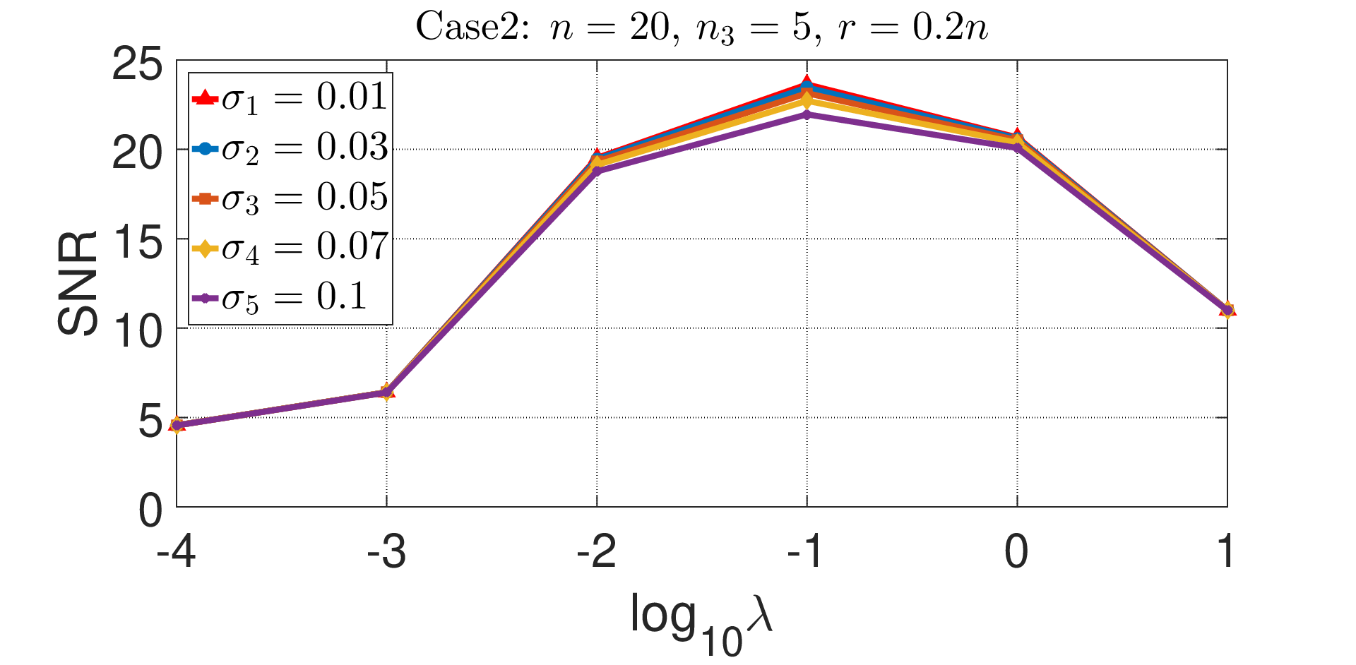
First, we generate a tubal rank rr tensor 𝓧∈ℝn×n×n3\boldsymbol{\mathcal{X}}\in\mathbb{R}^{n\times n\times n_{3}} as a product 𝓧=𝓧1∗𝓧2\boldsymbol{\mathcal{X}}=\boldsymbol{\mathcal{X}}_{1}\ast\boldsymbol{\mathcal{X}}_{2} where 𝓧1∈ℝn×r×n3\boldsymbol{\mathcal{X}}_{1}\in\mathbb{R}^{n\times r\times n_{3}} and 𝓧2∈ℝr×n×n3\boldsymbol{\mathcal{X}}_{2}\in\mathbb{R}^{r\times n\times n_{3}} are two tensors with entries independently sampled from a standard Gaussian distribution. Next, we generate a measurement matrix 𝑴∈ℝm×(n2​n3)\boldsymbol{M}\in\mathbb{R}^{m\times(n^{2}n_{3})} with i.i.d. 𝒩⁡(0,1/m)\mathcal{N}(0,1/m) entries. Using 𝓧\boldsymbol{\mathcal{X}} and 𝑴\boldsymbol{M}, the measurements 𝒚\boldsymbol{y} are produced by 𝒚=𝑴​vec​(𝓧)+𝐰\boldsymbol{y}=\boldsymbol{M}\rm vec(\boldsymbol{\mathcal{X}})+\boldsymbol{w}, where 𝒘\boldsymbol{w} is the Gaussian white noise with mean 00 and variance σ2\sigma^{2} (the greater σ\sigma, the greater the noise level ϵ\epsilon). We uniformly evaluate the recovery performance of the model by the signal-to-noise ratio (SNR) defined as 20​log⁡(‖𝓧‖F/‖𝓧−𝓧^‖F)20\log(\|\boldsymbol{\mathcal{X}}\|_{F}/\|\boldsymbol{\mathcal{X}}-\hat{\boldsymbol{\mathcal{X}}}\|_{F}) in decibels (dB) (the greater the SNR, the smaller the reconstruction error). The key to studying the RTNNM model (3) is to explain the relationship among reconstruction error, noise level ϵ\epsilon and λ\lambda. Therefore, we design three sets of experiments to explain it. Case 1: n=10n=10, n3=5n_{3}=5, r=0.1​nr=0.1n; Case 2: n=20n=20, n3=5n_{3}=5, r=0.2​nr=0.2n; Case 3: n=30n=30, n3=5n_{3}=5, r=0.3​nr=0.3n. According to [22], the number of samples in case 1 is set to 2​r​(2​n+1)​n32r(2n+1)n_{3}, and the number of samples in case 2 and 3 is set to 1.5​r​(2​n+1)​n31.5r(2n+1)n_{3}.

All SNR values for σ\sigma varying among {0.01,0.03,0.05,0.07,0.1}\{0.01,0.03,0.05,0.07,0.1\} and regularization parameters λ\lambda varying among {101,100,10−1,10−2,10−3,10−4}\{10^{1},10^{0},10^{-1},10^{-2},10^{-3},10^{-4}\} in three cases are provided in Table 1 with the best results highlighted in bold. It can be seen that there exist a consistent phenomenon for low-tubal-rank tensor recovery at different scales. When the regularization parameter λ=10−1\lambda=10^{-1}, as the standard deviation σ\sigma increases, the SNR gradually decreases. There is only a slight trend for other regularization parameters λ\lambda. In addition, for each fixed noise level, the regularization parameter λ=10−1\lambda=10^{-1} corresponds to the maximum SNR, which means the best of the low-tubal-rank tensor recovery. Therefore, λ=10−1\lambda=10^{-1} is the optimal regularization parameter of the RTNNM model (3) in three cases. We plot the data in Table 1 as Figure 2, which allows us to see the results of the above analysis at a glance. Thus, these experiments clearly demonstrate the quantitative correlation among reconstruction error, noise level ϵ\epsilon and λ\lambda.

Table 1: SNR for different noise levels and regularization parameters.
Case 1: n=10n=10, n3=5n_{3}=5, r=0.1​nr=0.1n
SNR (dB) σ1=0.01\sigma_{1}=0.01 σ2=0.03\sigma_{2}=0.03 σ3=0.05\sigma_{3}=0.05 σ4=0.07\sigma_{4}=0.07 σ5=0.1\sigma_{5}=0.1
λ1=101\lambda_{1}=10^{1} 12.0980 12.0981 12.0970 12.0948 12.0892
λ2=100\lambda_{2}=10^{0} 25.8704 25.7607 25.5490 25.2479 24.6683
λ3=10−1\lambda_{3}=10^{-1} 31.0711 30.4264 29.4052 28.2704 26.6232
λ4=10−2\lambda_{4}=10^{-2} 22.7064 22.5787 22.3462 22.0335 21.4687
λ5=10−3\lambda_{5}=10^{-3} 5.5688 5.5679 5.5660 5.5632 5.5573
λ6=10−4\lambda_{6}=10^{-4} 2.7720 2.7718 2.7713 2.7706 2.7691
Case 2: n=20n=20, n3=5n_{3}=5, r=0.2​nr=0.2n
SNR (dB) σ1=0.01\sigma_{1}=0.01 σ2=0.03\sigma_{2}=0.03 σ3=0.05\sigma_{3}=0.05 σ4=0.07\sigma_{4}=0.07 σ5=0.1\sigma_{5}=0.1
λ1=101\lambda_{1}=10^{1} 11.0030 11.0015 10.9986 10.9941 10.9845
λ2=100\lambda_{2}=10^{0} 20.6674 20.6139 20.5124 20.3671 20.0778
λ3=10−1\lambda_{3}=10^{-1} 23.6323 23.4598 23.1416 22.7156 21.9574
λ4=10−2\lambda_{4}=10^{-2} 19.5214 19.4528 19.3200 19.1312 18.7651
λ5=10−3\lambda_{5}=10^{-3} 6.4141 6.4128 6.4102 6.4065 6.3984
λ6=10−4\lambda_{6}=10^{-4} 4.5625 4.5620 4.5608 4.5591 4.5555
Case 3: n=30n=30, n3=5n_{3}=5, r=0.3​nr=0.3n
SNR (dB) σ1=0.01\sigma_{1}=0.01 σ2=0.03\sigma_{2}=0.03 σ3=0.05\sigma_{3}=0.05 σ4=0.07\sigma_{4}=0.07 σ5=0.1\sigma_{5}=0.1
λ1=101\lambda_{1}=10^{1} 14.7061 14.7034 14.6986 14.6917 14.6774
λ2=100\lambda_{2}=10^{0} 30.0564 29.8961 29.5879 29.1587 28.3575
λ3=10−1\lambda_{3}=10^{-1} 48.0263 41.8665 37.3142 33.9986 30.3401
λ4=10−2\lambda_{4}=10^{-2} 50.1381 38.8254 33.6326 30.2868 26.8153
λ5=10−3\lambda_{5}=10^{-3} 14.1284 14.1003 14.0445 13.9624 13.7947
λ6=10−4\lambda_{6}=10^{-4} 11.0540 11.0440 11.0242 10.9946 10.9324
Refer to caption
Refer to caption
Refer to caption
Figure 2: SNR for different noise levels and regularization parameters. (a) λ\lambda versus SNR with n=10n=10, n3=5n_{3}=5 and r=0.1​nr=0.1n. (b) λ\lambda versus SNR with n=20n=20, n3=5n_{3}=5 and r=0.2​nr=0.2n. (c) λ\lambda versus SNR with n=30n=30, n3=5n_{3}=5 and r=0.3​nr=0.3n.

5.3 Discussion

According to the established theoretical results in Theorem 4.1, to obtain an exact low tubal rank solution (i.e., the case when ϵ=0\epsilon=0 and 𝓧\boldsymbol{\mathcal{X}} is a tensor with tubal rank rr) of RTNNM model (3), one has to set λ\lambda to be 00. However, when it comes to the practice use, such a setting is obviously impossible. In fact, the practical wisdom (see, e.g., [33, 34, 35]) also indicates that the selection of λ\lambda may also be effected by the data scale, sampling number, approximation accuracy, objective function, low-rankness of the desired tensor, etc. On the other hand, if taking a closer look at the obtained theoretical results in the presence of noise (i.e., ϵ≠0\epsilon\neq 0), one will find that setting the lambda to be a sufficient big or small value is also not helpful to approach an expected approximate solution. In a word, one has to carefully select such a regularization parameter to obtained a desired optimal solution. This is exactly what we are trying to explain in our experiments.

6 Conclusion

In this paper, a heuristic notion of tensor Restricted Isometry Property (t-RIP) has been introduced based on tensor Singular Value Decomposition (t-SVD). Comparing with other definitions [11, 8], it is more representative as a higher-order generalization of the traditional RIP for vector and matrix recovery since the forms and properties of t-RIP and t-SVD are consistent with the vector/matrix case. This point is crucial because this guarantees that our theoretical investigation can be done in a similar way as CS and LRMR. A sufficient condition was presented, based on the RTNNM model, for stably recovering a given low-tubal-rank tensor that is corrupted with an ℓ2\ell_{2}-norm bounded noise. However, this condition only considers the δt​r𝕸\delta_{tr}^{\boldsymbol{\mathfrak{M}}} of the map 𝕸\boldsymbol{\mathfrak{M}} when tt is limited to t>1t>1. In the future, we hope to provide a complete answer for δt​r𝕸\delta_{tr}^{\boldsymbol{\mathfrak{M}}} when 0<t≤10<t\leq 1.

Acknowledgment

This work was supported by National Natural Science Foundation of China (Grant Nos. 61673015, 61273020), Fundamental Research Funds for the Central Universities (Grant Nos. XDJK2018C076, SWU1809002) and China Postdoctoral Science Foundation (Grant No. 2018M643390) and Graduate Student Scientific Research Innovation Projects in Chongqing (Grant No. CYB19083).

Appendix A Proof of Lemma 3.2

Proof.

Step 1: Sparse Representation of a Polytope.

Without loss of generality, assume that t​rtr is an integer for a given t>1t>1. Next we divide the index set Γc\Gamma^{c} into two disjoint subsets, that is,

Γ1={i∈Γc:𝓢𝓗​(i,i,1)>ϕ},Γ2={i∈Γc:𝓢𝓗​(i,i,1)≤ϕ},\Gamma_{1}=\{i\in\Gamma^{c}:\boldsymbol{\mathcal{S}}_{\boldsymbol{\mathcal{H}}}(i,i,1)>\phi\},~~\Gamma_{2}=\{i\in\Gamma^{c}:\boldsymbol{\mathcal{S}}_{\boldsymbol{\mathcal{H}}}(i,i,1)\leq\phi\},

where ϕ≜‖𝓗Γc‖∗/((t−1)​r)\phi\triangleq\|\boldsymbol{\mathcal{H}}_{\Gamma^{c}}\|_{*}/((t-1)r). Clearly,

Γ1∪Γ2=Γc​and​Γ1∩Γ=∅,\Gamma_{1}\cup\Gamma_{2}=\Gamma^{c}~\rm and~\Gamma_{1}\cap\Gamma=\emptyset,

which implies that 𝓗=𝓗Γ+𝓗Γc=𝓗Γ+𝓗Γ1+𝓗Γ2\boldsymbol{\mathcal{H}}=\boldsymbol{\mathcal{H}}_{\Gamma}+\boldsymbol{\mathcal{H}}_{\Gamma^{c}}=\boldsymbol{\mathcal{H}}_{\Gamma}+\boldsymbol{\mathcal{H}}_{\Gamma_{1}}+\boldsymbol{\mathcal{H}}_{\Gamma_{2}} and ‖𝓗Γ‖F≤‖𝓗Γ∪Γ1‖F\|\boldsymbol{\mathcal{H}}_{\Gamma}\|_{F}\leq\|\boldsymbol{\mathcal{H}}_{\Gamma\cup\Gamma_{1}}\|_{F}, respectively. In order to prove (8), we only need to check

‖𝓗Γ∪Γ1‖F≤η1​‖𝕸⁡(𝓗)‖2+η2r​‖𝓗Γc‖∗.\|\boldsymbol{\mathcal{H}}_{\Gamma\cup\Gamma_{1}}\|_{F}\leq\eta_{1}\|\boldsymbol{\mathfrak{M}}(\boldsymbol{\mathcal{H}})\|_{2}+\frac{\eta_{2}}{\sqrt{r}}\|\boldsymbol{\mathcal{H}}_{\Gamma^{c}}\|_{*}. (22)

Let ‖𝒔𝓗Γ1‖1≜∑i∈Γ1𝓢𝓗​(i,i,1)=‖𝓗Γ1‖∗\|\boldsymbol{s}_{\boldsymbol{\mathcal{H}}_{\Gamma_{1}}}\|_{1}\triangleq\sum_{i\in\Gamma_{1}}\boldsymbol{\mathcal{S}}_{\boldsymbol{\mathcal{H}}}(i,i,1)=\|\boldsymbol{\mathcal{H}}_{\Gamma_{1}}\|_{*}, where 𝒔𝓗Γ1\boldsymbol{s}_{\boldsymbol{\mathcal{H}}_{\Gamma_{1}}} is denoted as the diagonal vector of first frontal slice of 𝓢𝓗\boldsymbol{\mathcal{S}}_{\boldsymbol{\mathcal{H}}} whose element 𝓢𝓗Γ1​(i,i,1)=𝓢𝓗​(i,i,1)\boldsymbol{\mathcal{S}}_{\boldsymbol{\mathcal{H}}_{\Gamma_{1}}}(i,i,1)=\boldsymbol{\mathcal{S}}_{\boldsymbol{\mathcal{H}}}(i,i,1) for i∈Γ1i\in\Gamma_{1} and 𝓢𝓗Γ1​(i,i,1)=0\boldsymbol{\mathcal{S}}_{\boldsymbol{\mathcal{H}}_{\Gamma_{1}}}(i,i,1)=0 otherwise. Since all non-zero entries of vector 𝒔𝓗Γ1\boldsymbol{s}_{\boldsymbol{\mathcal{H}}_{\Gamma_{1}}} have magnitude larger than ϕ\phi, we have,

‖𝒔𝓗Γ1‖1=‖𝓗Γ1‖∗>|Γ1|​‖𝓗Γc‖∗(t−1)​r≥|Γ1|​‖𝓗Γ1‖∗(t−1)​r=|Γ1|(t−1)​r​‖𝒔𝓗Γ1‖1.\|\boldsymbol{s}_{\boldsymbol{\mathcal{H}}_{\Gamma_{1}}}\|_{1}=\|\boldsymbol{\mathcal{H}}_{\Gamma_{1}}\|_{*}>|\Gamma_{1}|\frac{\|\boldsymbol{\mathcal{H}}_{\Gamma^{c}}\|_{*}}{(t-1)r}\geq|\Gamma_{1}|\frac{\|\boldsymbol{\mathcal{H}}_{\Gamma_{1}}\|_{*}}{(t-1)r}=\frac{|\Gamma_{1}|}{(t-1)r}\|\boldsymbol{s}_{\boldsymbol{\mathcal{H}}_{\Gamma_{1}}}\|_{1}.

Namely |Γ1|<(t−1)​r|\Gamma_{1}|<(t-1)r. Besides, we also have

‖𝒔𝓗Γ2‖1=‖𝓗Γ2‖∗=‖𝓗Γc‖∗−‖𝓗Γ1‖∗≤((t−1)​r−|Γ1|)​ϕ\|\boldsymbol{s}_{\boldsymbol{\mathcal{H}}_{\Gamma_{2}}}\|_{1}=\|\boldsymbol{\mathcal{H}}_{\Gamma_{2}}\|_{*}=\|\boldsymbol{\mathcal{H}}_{\Gamma^{c}}\|_{*}-\|\boldsymbol{\mathcal{H}}_{\Gamma_{1}}\|_{*}\leq((t-1)r-|\Gamma_{1}|)\phi

and

‖𝒔𝓗Γ2‖∞≜maxi∈Γ2⁡𝓢𝓗​(i,i,1)≤ϕ.\|\boldsymbol{s}_{\boldsymbol{\mathcal{H}}_{\Gamma_{2}}}\|_{\infty}\triangleq\max_{i\in\Gamma_{2}}\boldsymbol{\mathcal{S}}_{\boldsymbol{\mathcal{H}}}(i,i,1)\leq\phi.

Now, since 𝒔𝓗Γ2∈T⁡(ϕ,(t−1)​r−|Γ1|)\boldsymbol{s}_{\boldsymbol{\mathcal{H}}_{\Gamma_{2}}}\in T(\phi,(t-1)r-|\Gamma_{1}|), applying Lemma 3.1, 𝒔𝓗Γ2\boldsymbol{s}_{\boldsymbol{\mathcal{H}}_{\Gamma_{2}}} can be rewritten as:

𝒔𝓗Γ2=∑i=1Nγi​𝒈i,\boldsymbol{s}_{\boldsymbol{\mathcal{H}}_{\Gamma_{2}}}=\sum_{i=1}^{N}\gamma_{i}\boldsymbol{g}_{i},

where 𝒈i∈U⁡(ϕ,(t−1)​r−|Γ1|,𝒔𝓗Γ2)\boldsymbol{g}_{i}\in U(\phi,(t-1)r-|\Gamma_{1}|,\boldsymbol{s}_{\boldsymbol{\mathcal{H}}_{\Gamma_{2}}}) and 0≤γi≤10\leq\gamma_{i}\leq 1, ∑i=1Nγi=1\sum_{i=1}^{N}\gamma_{i}=1.

Step 2: Consequence of t-RIP.

Furthermore, define

𝒔𝓑i\displaystyle\boldsymbol{s}_{\boldsymbol{\mathcal{B}}_{i}} =\displaystyle= (1+δt​r𝕸)​𝒔𝓗Γ∪Γ1+δt​r𝕸​𝒔𝓖i,𝒔𝓟i=(1−δt​r𝕸)​𝒔𝓗Γ∪Γ1−δt​r𝕸​𝒔𝓖i,\displaystyle(1+\delta_{tr}^{\boldsymbol{\mathfrak{M}}})\boldsymbol{s}_{\boldsymbol{\mathcal{H}}_{\Gamma\cup\Gamma_{1}}}+\delta_{tr}^{\boldsymbol{\mathfrak{M}}}\boldsymbol{s}_{\boldsymbol{\mathcal{G}}_{i}},\quad\boldsymbol{s}_{\boldsymbol{\mathcal{P}}_{i}}=(1-\delta_{tr}^{\boldsymbol{\mathfrak{M}}})\boldsymbol{s}_{\boldsymbol{\mathcal{H}}_{\Gamma\cup\Gamma_{1}}}-\delta_{tr}^{\boldsymbol{\mathfrak{M}}}\boldsymbol{s}_{\boldsymbol{\mathcal{G}}_{i}},
𝓖i\displaystyle\boldsymbol{\mathcal{G}}_{i} =\displaystyle= ∑j=1κ𝓤𝓗(:,j,:)∗𝓢𝓖i(j,j,:)∗𝓥𝓗(:,j,:)∗,\displaystyle\sum\nolimits_{j=1}^{\kappa}\boldsymbol{\mathcal{U}}_{\boldsymbol{\mathcal{H}}}(:,j,:)\ast\boldsymbol{\mathcal{S}}_{\boldsymbol{\mathcal{G}}_{i}}(j,j,:)\ast\boldsymbol{\mathcal{V}}_{\boldsymbol{\mathcal{H}}}(:,j,:)^{*},
𝓑i\displaystyle\boldsymbol{\mathcal{B}}_{i} =\displaystyle= ∑j=1κ𝓤𝓗(:,j,:)∗𝓢𝓑i(j,j,:)∗𝓥𝓗(:,j,:)∗,\displaystyle\sum\nolimits_{j=1}^{\kappa}\boldsymbol{\mathcal{U}}_{\boldsymbol{\mathcal{H}}}(:,j,:)\ast\boldsymbol{\mathcal{S}}_{\boldsymbol{\mathcal{B}}_{i}}(j,j,:)\ast\boldsymbol{\mathcal{V}}_{\boldsymbol{\mathcal{H}}}(:,j,:)^{*},
𝓟i\displaystyle\boldsymbol{\mathcal{P}}_{i} =\displaystyle= ∑j=1κ𝓤𝓗(:,j,:)∗𝓢𝓟i(j,j,:)∗𝓥𝓗(:,j,:)∗.\displaystyle\sum\nolimits_{j=1}^{\kappa}\boldsymbol{\mathcal{U}}_{\boldsymbol{\mathcal{H}}}(:,j,:)\ast\boldsymbol{\mathcal{S}}_{\boldsymbol{\mathcal{P}}_{i}}(j,j,:)\ast\boldsymbol{\mathcal{V}}_{\boldsymbol{\mathcal{H}}}(:,j,:)^{*}.

Then it is not hard to see that both 𝑩i\boldsymbol{B}_{i} and 𝑷i\boldsymbol{P}_{i} are all tensors with tubal rank at most t​rtr for i=1,2,⋯,Ni=1,2,\cdots,N, and

𝓗Γ2=∑i=1Nγi​𝓖i,𝓑i=(1+δt​r𝕸)​𝓗Γ∪Γ1+δt​r𝕸​𝓖i,𝓟i=(1−δt​r𝕸)​𝓗Γ∪Γ1−δt​r𝕸​𝓖i.\boldsymbol{\mathcal{H}}_{\Gamma_{2}}=\sum\nolimits_{i=1}^{N}\gamma_{i}\boldsymbol{\mathcal{G}}_{i},~~\boldsymbol{\mathcal{B}}_{i}=(1+\delta_{tr}^{\boldsymbol{\mathfrak{M}}})\boldsymbol{\mathcal{H}}_{\Gamma\cup\Gamma_{1}}+\delta_{tr}^{\boldsymbol{\mathfrak{M}}}\boldsymbol{\mathcal{G}}_{i},~~\boldsymbol{\mathcal{P}}_{i}=(1-\delta_{tr}^{\boldsymbol{\mathfrak{M}}})\boldsymbol{\mathcal{H}}_{\Gamma\cup\Gamma_{1}}-\delta_{tr}^{\boldsymbol{\mathfrak{M}}}\boldsymbol{\mathcal{G}}_{i}.

Now we estimate the upper bounds of

ξ≜∑i=1Nγi​(‖𝕸⁡(𝓑i)‖22−‖𝕸⁡(𝓟i)‖22).\xi\triangleq\sum\nolimits_{i=1}^{N}\gamma_{i}\left(\|\boldsymbol{\mathfrak{M}}(\boldsymbol{\mathcal{B}}_{i})\|_{2}^{2}-\|\boldsymbol{\mathfrak{M}}(\boldsymbol{\mathcal{P}}_{i})\|_{2}^{2}\right).

Applying Definition 1.1, we have

ξ\displaystyle\xi =\displaystyle= 4​δt​r𝕸​∑i=1Nγi​⟨𝕸⁡(𝓗Γ∪Γ1),𝕸⁡(𝓗Γ∪Γ1+𝓖i)⟩\displaystyle 4\delta_{tr}^{\boldsymbol{\mathfrak{M}}}\sum\nolimits_{i=1}^{N}\gamma_{i}\left\langle\boldsymbol{\mathfrak{M}}(\boldsymbol{\mathcal{H}}_{\Gamma\cup\Gamma_{1}}),\boldsymbol{\mathfrak{M}}(\boldsymbol{\mathcal{H}}_{\Gamma\cup\Gamma_{1}}+\boldsymbol{\mathcal{G}}_{i})\right\rangle (23)
=(a)\displaystyle\stackrel{{\scriptstyle(a)}}{{=}} 4​δt​r𝕸​⟨𝕸⁡(𝓗Γ∪Γ1),𝕸⁡(𝓗Γ∪Γ1+∑i=1Nγi​𝓖i)⟩\displaystyle 4\delta_{tr}^{\boldsymbol{\mathfrak{M}}}\left\langle\boldsymbol{\mathfrak{M}}(\boldsymbol{\mathcal{H}}_{\Gamma\cup\Gamma_{1}}),\boldsymbol{\mathfrak{M}}\left(\boldsymbol{\mathcal{H}}_{\Gamma\cup\Gamma_{1}}+\sum\nolimits_{i=1}^{N}\gamma_{i}\boldsymbol{\mathcal{G}}_{i}\right)\right\rangle
=(b)\displaystyle\stackrel{{\scriptstyle(b)}}{{=}} 4​δt​r𝕸​⟨𝕸⁡(𝓗Γ∪Γ1),𝕸⁡(𝓗)⟩\displaystyle 4\delta_{tr}^{\boldsymbol{\mathfrak{M}}}\langle\boldsymbol{\mathfrak{M}}(\boldsymbol{\mathcal{H}}_{\Gamma\cup\Gamma_{1}}),\boldsymbol{\mathfrak{M}}(\boldsymbol{\mathcal{H}})\rangle
≤(c)\displaystyle\stackrel{{\scriptstyle(c)}}{{\leq}} 4​δt​r𝕸​‖𝕸⁡(𝓗Γ∪Γ1)‖2​‖𝕸⁡(𝓗)‖2\displaystyle 4\delta_{tr}^{\boldsymbol{\mathfrak{M}}}\|\boldsymbol{\mathfrak{M}}(\boldsymbol{\mathcal{H}}_{\Gamma\cup\Gamma_{1}})\|_{2}\|\boldsymbol{\mathfrak{M}}(\boldsymbol{\mathcal{H}})\|_{2}
≤(d)\displaystyle\stackrel{{\scriptstyle(d)}}{{\leq}} 4​δt​r𝕸​1+δt​r𝕸​‖𝓗Γ∪Γ1‖F​‖𝕸⁡(𝓗)‖2,\displaystyle 4\delta_{tr}^{\boldsymbol{\mathfrak{M}}}\sqrt{1+\delta_{tr}^{\boldsymbol{\mathfrak{M}}}}\|\boldsymbol{\mathcal{H}}_{\Gamma\cup\Gamma_{1}}\|_{F}\|\boldsymbol{\mathfrak{M}}(\boldsymbol{\mathcal{H}})\|_{2},

where (a) is due to ∑i=1Nγi=1\sum_{i=1}^{N}\gamma_{i}=1, (b) is founded on the fact that 𝓗Γ2=∑i=1Nγi​𝓖i\boldsymbol{\mathcal{H}}_{\Gamma_{2}}=\sum\nolimits_{i=1}^{N}\gamma_{i}\boldsymbol{\mathcal{G}}_{i} and 𝓗=𝓗Γ+𝓗Γ1+𝓗Γ2\boldsymbol{\mathcal{H}}=\boldsymbol{\mathcal{H}}_{\Gamma}+\boldsymbol{\mathcal{H}}_{\Gamma_{1}}+\boldsymbol{\mathcal{H}}_{\Gamma_{2}}, (c) holds because of the Cauchy-Schwartz inequality, and (d) follows from (4), |Γ1|<(t−1)​r|\Gamma_{1}|<(t-1)r and the monotonicity of t-RIC.

Next, we use the block diagonal matrix to estimate the lower bound of ξ\xi. Let ϕ¯≜‖bdiag(𝓗¯Γc)‖∗/(t−1)​r\bar{\phi}\triangleq\|\mathop{\rm bdiag}(\boldsymbol{\bar{\mathcal{H}}}_{\Gamma^{c}})\|_{*}/(t-1)r. Repeat step 1 for the matrix bdiag(𝓗¯)\mathop{\rm bdiag}(\boldsymbol{\bar{\mathcal{H}}}) as we did for tensor 𝓗\boldsymbol{\mathcal{H}} and we have

σ⁡(bdiag(𝓗¯Γ2))∈T⁡(ϕ¯,(t−1)​r−|E1|),𝒈¯i∈U⁡(ϕ¯,(t−1)​r−|E1|,σ⁡(bdiag(𝓗¯Γ2))),\sigma(\mathop{\rm bdiag}(\boldsymbol{\bar{\mathcal{H}}}_{\Gamma_{2}}))\in T(\bar{\phi},(t-1)r-|E_{1}|),~~\boldsymbol{\bar{g}}_{i}\in U(\bar{\phi},(t-1)r-|E_{1}|,\sigma(\mathop{\rm bdiag}(\boldsymbol{\bar{\mathcal{H}}}_{\Gamma_{2}}))),

here, E1E_{1} is an index set as the counterpart of Γ1\Gamma_{1}. By further defining

𝒃¯i\displaystyle\boldsymbol{\bar{b}}_{i} =\displaystyle= (1+δt​r𝕸)​σ​(bdiag(𝓗¯Γ∪Γ1))+δt​r𝕸​𝒈¯i,\displaystyle(1+\delta_{tr}^{\boldsymbol{\mathfrak{M}}})\sigma(\mathop{\rm bdiag}(\boldsymbol{\bar{\mathcal{H}}}_{\Gamma\cup\Gamma_{1}}))+\delta_{tr}^{\boldsymbol{\mathfrak{M}}}\boldsymbol{\bar{g}}_{i},
𝒑¯i\displaystyle\boldsymbol{\bar{p}}_{i} =\displaystyle= (1−δt​r𝕸)​σ​(bdiag(𝓗¯Γ∪Γ1))−δt​r𝕸​𝒈¯i,\displaystyle(1-\delta_{tr}^{\boldsymbol{\mathfrak{M}}})\sigma(\mathop{\rm bdiag}(\boldsymbol{\bar{\mathcal{H}}}_{\Gamma\cup\Gamma_{1}}))-\delta_{tr}^{\boldsymbol{\mathfrak{M}}}\boldsymbol{\bar{g}}_{i},
𝑮¯i\displaystyle\boldsymbol{\bar{G}}_{i} =\displaystyle= ∑j=1κ(𝒖𝑯¯)j⋅(𝒈¯i)j⋅(𝒗𝑯¯)j∗,\displaystyle\sum\nolimits_{j=1}^{\kappa}(\boldsymbol{u}_{\boldsymbol{\bar{H}}})_{j}\cdot(\boldsymbol{\bar{g}}_{i})_{j}\cdot(\boldsymbol{v}_{\boldsymbol{\bar{H}}})_{j}^{*},
𝑩¯i\displaystyle\boldsymbol{\bar{B}}_{i} =\displaystyle= ∑j=1κ(𝒖𝑯¯)j⋅(𝒃¯i)j⋅(𝒗𝑯¯)j∗,\displaystyle\sum\nolimits_{j=1}^{\kappa}(\boldsymbol{u}_{\boldsymbol{\bar{H}}})_{j}\cdot(\boldsymbol{\bar{b}}_{i})_{j}\cdot(\boldsymbol{v}_{\boldsymbol{\bar{H}}})_{j}^{*},
𝑷¯i\displaystyle\boldsymbol{\bar{P}}_{i} =\displaystyle= ∑j=1κ(𝒖𝑯¯)j⋅(𝒑¯i)j⋅(𝒗𝑯¯)j∗.\displaystyle\sum\nolimits_{j=1}^{\kappa}(\boldsymbol{u}_{\boldsymbol{\bar{H}}})_{j}\cdot(\boldsymbol{\bar{p}}_{i})_{j}\cdot(\boldsymbol{v}_{\boldsymbol{\bar{H}}})_{j}^{*}.

Then we can easily induce that

bdiag(𝓗¯Γ2)\displaystyle\mathop{\rm bdiag}(\boldsymbol{\bar{\mathcal{H}}}_{\Gamma_{2}}) =\displaystyle= ∑i=1Nγi​𝑮¯i,\displaystyle\sum\nolimits_{i=1}^{N}\gamma_{i}\boldsymbol{\bar{G}}_{i},
𝑩¯i\displaystyle\boldsymbol{\bar{B}}_{i} =\displaystyle= (1+δt​r𝕸)​bdiag(𝓗¯Γ∪Γ1)+δt​r𝕸​𝑮¯i,\displaystyle(1+\delta_{tr}^{\boldsymbol{\mathfrak{M}}})\mathop{\rm bdiag}(\boldsymbol{\bar{\mathcal{H}}}_{\Gamma\cup\Gamma_{1}})+\delta_{tr}^{\boldsymbol{\mathfrak{M}}}\boldsymbol{\bar{G}}_{i},
𝑷¯i\displaystyle\boldsymbol{\bar{P}}_{i} =\displaystyle= (1−δt​r𝕸)​bdiag(𝓗¯Γ∪Γ1)−δt​r𝕸​𝑮¯i.\displaystyle(1-\delta_{tr}^{\boldsymbol{\mathfrak{M}}})\mathop{\rm bdiag}(\boldsymbol{\bar{\mathcal{H}}}_{\Gamma\cup\Gamma_{1}})-\delta_{tr}^{\boldsymbol{\mathfrak{M}}}\boldsymbol{\bar{G}}_{i}.

Thus, on the other hand, we also have

ξ\displaystyle\xi ≥(a)\displaystyle\stackrel{{\scriptstyle(a)}}{{\geq}} ∑i=1Nγi​((1−δt​r𝕸)​‖𝓑i‖F2−(1+δt​r𝕸)​‖𝓟i‖F2)\displaystyle\sum\nolimits_{i=1}^{N}\gamma_{i}\left((1-\delta_{tr}^{\boldsymbol{\mathfrak{M}}})\|\boldsymbol{\mathcal{B}}_{i}\|_{F}^{2}-(1+\delta_{tr}^{\boldsymbol{\mathfrak{M}}})\|\boldsymbol{\mathcal{P}}_{i}\|_{F}^{2}\right) (24)
=(b)\displaystyle\stackrel{{\scriptstyle(b)}}{{=}} 1n3​∑i=1Nγi​((1−δt​r𝕸)​‖𝑩¯i‖22−(1+δt​r𝕸)​‖𝑷¯i‖22)\displaystyle\frac{1}{n_{3}}\sum\nolimits_{i=1}^{N}\gamma_{i}\left((1-\delta_{tr}^{\boldsymbol{\mathfrak{M}}})\|\boldsymbol{\bar{B}}_{i}\|_{2}^{2}-(1+\delta_{tr}^{\boldsymbol{\mathfrak{M}}})\|\boldsymbol{\bar{P}}_{i}\|_{2}^{2}\right)
=(c)\displaystyle\stackrel{{\scriptstyle(c)}}{{=}} 2n3​δt​r𝕸​(1−(δt​r𝕸)2)​‖σ⁡(bdiag(𝓗¯Γ∪Γ1))‖22−2n3​(δt​r𝕸)3​∑i=1Nγi​‖𝒈¯i‖22\displaystyle\frac{2}{n_{3}}\delta_{tr}^{\boldsymbol{\mathfrak{M}}}(1-(\delta_{tr}^{\boldsymbol{\mathfrak{M}}})^{2})\|\sigma(\mathop{\rm bdiag}(\boldsymbol{\bar{\mathcal{H}}}_{\Gamma\cup\Gamma_{1}}))\|_{2}^{2}-\frac{2}{n_{3}}(\delta_{tr}^{\boldsymbol{\mathfrak{M}}})^{3}\sum\nolimits_{i=1}^{N}\gamma_{i}\|\boldsymbol{\bar{g}}_{i}\|_{2}^{2}
≥(d)\displaystyle\stackrel{{\scriptstyle(d)}}{{\geq}} 2n3​δt​r𝕸​(1−(δt​r𝕸)2)​‖bdiag(𝓗¯Γ∪Γ1)‖F2−2​(δt​r𝕸)3n3​(t−1)​r​‖bdiag(𝓗¯Γc)‖∗2\displaystyle\frac{2}{n_{3}}\delta_{tr}^{\boldsymbol{\mathfrak{M}}}(1-(\delta_{tr}^{\boldsymbol{\mathfrak{M}}})^{2})\|\mathop{\rm bdiag}(\boldsymbol{\bar{\mathcal{H}}}_{\Gamma\cup\Gamma_{1}})\|_{F}^{2}-\frac{2(\delta_{tr}^{\boldsymbol{\mathfrak{M}}})^{3}}{n_{3}(t-1)r}\|\mathop{\rm bdiag}(\boldsymbol{\bar{\mathcal{H}}}_{\Gamma^{c}})\|_{*}^{2}
=(e)\displaystyle\stackrel{{\scriptstyle(e)}}{{=}} 2​δt​r𝕸​(1−(δt​r𝕸)2)​‖𝓗Γ∪Γ1‖F2−2​n3​(δt​r𝕸)3(t−1)​r​‖𝓗Γc‖∗2,\displaystyle 2\delta_{tr}^{\boldsymbol{\mathfrak{M}}}(1-(\delta_{tr}^{\boldsymbol{\mathfrak{M}}})^{2})\|\boldsymbol{\mathcal{H}}_{\Gamma\cup\Gamma_{1}}\|_{F}^{2}-\frac{2n_{3}(\delta_{tr}^{\boldsymbol{\mathfrak{M}}})^{3}}{(t-1)r}\|\boldsymbol{\mathcal{H}}_{\Gamma^{c}}\|_{*}^{2},

where (a) follows from t-RIP, (b) holds because of (5), (c) is due to ⟨σ⁡(bdiag(𝓗¯Γ∪Γ1)),𝒈¯i⟩=0\langle\sigma(\mathop{\rm bdiag}(\boldsymbol{\bar{\mathcal{H}}}_{\Gamma\cup\Gamma_{1}})),\boldsymbol{\bar{g}}_{i}\rangle=0 for all i=1,2,⋯,Ni=1,2,\cdots,N, (d) is based on the fact that ‖𝑿‖F=‖σ⁡(𝑿)‖2\|\boldsymbol{X}\|_{F}=\|\sigma(\boldsymbol{X})\|_{2} for any matrix 𝑿\boldsymbol{X} and

‖𝒈¯i‖22≤‖𝒈¯i‖0​(‖𝒈¯i‖∞)2≤((t−1)​r−|E1|)​ϕ¯2≤‖bdiag(𝓗¯Γc)‖∗2(t−1)​r,\|\boldsymbol{\bar{g}}_{i}\|_{2}^{2}\leq\|\boldsymbol{\bar{g}}_{i}\|_{0}(\|\boldsymbol{\bar{g}}_{i}\|_{\infty})^{2}\leq((t-1)r-|E_{1}|)\bar{\phi}^{2}\leq\frac{\|\mathop{\rm bdiag}(\boldsymbol{\bar{\mathcal{H}}}_{\Gamma^{c}})\|_{*}^{2}}{(t-1)r},

and (e) follows from (6).

Combining (23) and (24), we get

(1−(δt​r𝕸)2)​‖𝓗Γ∪Γ1‖F2−n3​(δt​r𝕸)2(t−1)​r​‖𝓗Γc‖∗2≤2​1+δt​r𝕸​‖𝓗Γ∪Γ1‖F​‖𝕸⁡(𝓗)‖2.(1-(\delta_{tr}^{\boldsymbol{\mathfrak{M}}})^{2})\|\boldsymbol{\mathcal{H}}_{\Gamma\cup\Gamma_{1}}\|_{F}^{2}-\frac{n_{3}(\delta_{tr}^{\boldsymbol{\mathfrak{M}}})^{2}}{(t-1)r}\|\boldsymbol{\mathcal{H}}_{\Gamma^{c}}\|_{*}^{2}\leq 2\sqrt{1+\delta_{tr}^{\boldsymbol{\mathfrak{M}}}}\|\boldsymbol{\mathcal{H}}_{\Gamma\cup\Gamma_{1}}\|_{F}\|\boldsymbol{\mathfrak{M}}(\boldsymbol{\mathcal{H}})\|_{2}. (25)

Obviously, (25) is a quadratic inequality in terms of ‖𝓗Γ∪Γ1‖F\|\boldsymbol{\mathcal{H}}_{\Gamma\cup\Gamma_{1}}\|_{F}. Using extract roots formula, we obtain

‖𝓗Γ∪Γ1‖F\displaystyle\|\boldsymbol{\mathcal{H}}_{\Gamma\cup\Gamma_{1}}\|_{F}
≤\displaystyle\leq 2​1+δt​r𝕸​‖𝕸⁡(𝓗)‖2+(2​1+δt​r𝕸​‖𝕸⁡(𝓗)‖2)2+4​(1−(δt​r𝕸)2)​n3​(δt​r𝕸)2(t−1)​r​‖𝓗Γc‖∗22​(1−(δt​r𝕸)2)\displaystyle\frac{2\sqrt{1+\delta_{tr}^{\boldsymbol{\mathfrak{M}}}}\|\boldsymbol{\mathfrak{M}}(\boldsymbol{\mathcal{H}})\|_{2}+\sqrt{(2\sqrt{1+\delta_{tr}^{\boldsymbol{\mathfrak{M}}}}\|\boldsymbol{\mathfrak{M}}(\boldsymbol{\mathcal{H}})\|_{2})^{2}+4(1-(\delta_{tr}^{\boldsymbol{\mathfrak{M}}})^{2})\frac{n_{3}(\delta_{tr}^{\boldsymbol{\mathfrak{M}}})^{2}}{(t-1)r}\|\boldsymbol{\mathcal{H}}_{\Gamma^{c}}\|_{*}^{2}}}{2(1-(\delta_{tr}^{\boldsymbol{\mathfrak{M}}})^{2})}
≤\displaystyle\leq 2(1−δt​r𝕸)​1+δt​r𝕸​‖𝕸⁡(𝓗)‖2+n3​δt​r𝕸(1−(δt​r𝕸)2)​(t−1)​‖𝓗Γc‖∗r,\displaystyle\frac{2}{(1-\delta_{tr}^{\boldsymbol{\mathfrak{M}}})\sqrt{1+\delta_{tr}^{\boldsymbol{\mathfrak{M}}}}}\|\boldsymbol{\mathfrak{M}}(\boldsymbol{\mathcal{H}})\|_{2}+\frac{\sqrt{n_{3}}\delta_{tr}^{\boldsymbol{\mathfrak{M}}}}{\sqrt{(1-(\delta_{tr}^{\boldsymbol{\mathfrak{M}}})^{2})(t-1)}}\frac{\|\boldsymbol{\mathcal{H}}_{\Gamma^{c}}\|_{*}}{\sqrt{r}},

where the last inequality is based on the fact that x2+y2≤|x|+|y|\sqrt{x^{2}+y^{2}}\leq|x|+|y|. Therefore we prove (22). Since we also have ∥𝓗∥F≤∥𝓗Γ∪Γ1∥F\|\boldsymbol{\mathcal{H}}\|_{F}\leq\|\boldsymbol{\mathcal{H}}_{\Gamma\cup\Gamma_{1}\|_{F}}, it is easy to induce (8).

When t​rtr is not an integer, let t′=⌈t​r⌉/rt^{\prime}=\lceil tr\rceil/r, then t′​rt^{\prime}r is an integer. Based on the definition of t-RIP and t​r<⌈t​r⌉<t​r+1tr<\lceil tr\rceil<tr+1, we have δt′​r=δt​r<1\delta_{t^{\prime}r}=\delta_{tr}<1. Thus (8) holds no matter whether t​rtr is an integer or not. This completes the proof. ∎

References

  • [1] J. Liu, P. Musialski, P. Wonka, J. Ye, Tensor completion for estimating missing values in visual data, IEEE Trans. Pattern Anal. Mach. 35 (1) (2013) 208–220.
  • [2] A. Wang, X. Song, X. Wu, Z. Lai, Z. Jin, Generalized dantzig selector for low-tubal-rank tensor recovery, in: ICASSP, IEEE, Brighton, 2019, pp. 3427–3431.
  • [3] B. Romera-Paredes, H. Aung, N. Bianchi-Berthouze, M. Pontil, Multilinear multitask learning, in: Int. Conf. on Machine Learning, Proceedings of Machine Learning Research, Atlanta, 2013, pp. 1444–1452.
  • [4] Y. Wang, L. Lin, Q. Zhao, T. Yue, D. Meng, Y. Leung, Compressive sensing of hyperspectral images via joint tensor tucker decomposition and weighted total variation regularization, IEEE Geosci. Remote Sens. Lett. 14 (12) (2017) 2457–2461.
  • [5] M. Mørup, Applications of tensor (multiway array) factorizations and decompositions in data mining, Wiley Interdiscip. Rev.-Data Mining Knowl. Discov. 1 (1) (2011) 24–40.
  • [6] S. Friedland, Q. Li, D. Schonfeld, Compressive sensing of sparse tensors, IEEE Trans. Image Process. 23 (10) (2014) 4438–4447.
  • [7] C. Lu, J. Feng, W. Liu, Z. Lin, S. Yan, Tensor robust principal component analysis with a new tensor nuclear norm, IEEE Trans. Pattern Anal. Mach. Intell. 2019.
  • [8] H. Rauhut, R. Schneider, Ž. Stojanac, Low rank tensor recovery via iterative hard thresholding, Linear Alg. Appl. 523 (2017) 220–262.
  • [9] Z. Zhang, G. Ely, S. Aeron, N. Hao, M. Kilmer, Novel methods for multilinear data completion and de-noising based on tensor-svd, in: Proc. CVPR, IEEE, Columbus, 2014, pp. 3842–3849.
  • [10] C. Lu, J. Feng, Z. Lin, S. Yan, Exact low tubal rank tensor recovery from gaussian measurements, in: IJCAI, AAAI, Stockholm, 2018, pp. 2504–2510.
  • [11] Z. Shi, J. Han, T. Zheng, J. Li, Guarantees of augmented trace norm models in tensor recovery, in: IJCAI, AAAI, Beijing, 2013, pp. 1670–1676.
  • [12] H. A. Kiers, Towards a standardized notation and terminology in multiway analysis, J. Chemometr. 14 (3) (2000) 105–122.
  • [13] L. R. Tucker, Some mathematical notes on three-mode factor analysis, Psychometrika 31 (3) (1966) 279–311.
  • [14] C. Mu, B. Huang, J. Wright, D. Goldfarb, Square deal: Lower bounds and improved relaxations for tensor recovery, in: Int. Conf. on Machine Learning, Proceedings of Machine Learning Research, Beijing, 2014, pp. 73–81.
  • [15] M. E. Kilmer, C. D. Martin, Factorization strategies for third-order tensors, Linear Alg. Appl. 435 (3) (2011) 641–658.
  • [16] C. D. Martin, R. Shafer, B. LaRue, An order-p tensor factorization with applications in imaging, SIAM J. Sci. Comput. 35 (1) (2013) A474–A490.
  • [17] M. E. Kilmer, K. Braman, N. Hao, R. C. Hoover, Third-order tensors as operators on matrices: A theoretical and computational framework with applications in imaging, SIAM J. Matrix Anal. Appl. 34 (1) (2013) 148–172.
  • [18] H. Zhang, M. Yan, W. Yin, One condition for solution uniqueness and robustness of both l1-synthesis and l1-analysis minimizations, Adv. Comput. Math. 42 (6) (2016) 1381–1399.
  • [19] S. Boyd, N. Parikh, E. Chu, B. Peleato, J. Eckstein, et al., Distributed optimization and statistical learning via the alternating direction method of multipliers, Foundations and Trends in Machine learning 3 (1) (2011) 1–122.
  • [20] E. J. Cande`\grave{e}s, T. Tao, Decoding by linear programming, IEEE Trans. Inf. Theory 51 (12) (2005) 4203–4215.
  • [21] B. Recht, M. Fazel, P. A. Parrilo, Guaranteed minimum-rank solutions of linear matrix equations via nuclear norm minimization, SIAM Rev. 52 (3) (2010) 471–501.
  • [22] F. Zhang, W. Wang, J. Hou, J. Wang, J. Huang, Tensor restricted isometry property analysis for a large class of random measurement ensembles, arXiv preprint arXiv:1906.01198.
  • [23] E. J. Cande`\grave{e}s, The restricted isometry property and its implications for compressed sensing, C. R. Math. 346 (9) (2008) 589–592.
  • [24] E. J. Cande`\grave{e}s, Y. Plan, Tight oracle inequalities for low-rank matrix recovery from a minimal number of noisy random measurements, IEEE Trans. Inf. Theory 57 (4) (2011) 2342–2359.
  • [25] T. T. Cai, A. Zhang, Sharp rip bound for sparse signal and low-rank matrix recovery, Appl. Comput. Harmon. Anal. 35 (1) (2013) 74–93.
  • [26] T. T. Cai, A. Zhang, Sparse representation of a polytope and recovery of sparse signals and low-rank matrices, IEEE Trans. Inf. Theory 60 (1) (2014) 122–132.
  • [27] R. Zhang, S. Li, A proof of conjecture on restricted isometry property constants δt​k​(0<t<4/3)\delta_{tk}(0<t<4/3), IEEE Trans. Inf. Theory 64 (3) (2018) 1699–1705.
  • [28] C. Zhu, Stable recovery of sparse signals via regularized minimization, IEEE Trans. Inf. Theory 54 (7) (2008) 3364–3367.
  • [29] Y. Shen, B. Han, E. Braverman, Stable recovery of analysis based approaches, Appl. Comput. Harmon. Anal. 39 (1) (2015) 161–172.
  • [30] H. Ge, J. Wen, W. Chen, J. Weng, M.-J. Lai, Stable sparse recovery with three unconstrained analysis based approaches, http://alpha.math.uga.edu/mjlai/papers/20180126.pdf (2018).
  • [31] W. Wang, F. Zhang, J. Wang, Low-rank matrix recovery via regularized nuclear norm minimization (2019). arXiv:1903.01053.
  • [32] S. Foucart, Stability and robustness of ℓ1\ell_{1}-minimizations with weibull matrices and redundant dictionaries, Linear Alg. Appl. 441 (2014) 4–21.
  • [33] M. Lai, Y. Xu, W. Yin, Improved iteratively reweighted least squares for unconstrained smoothed ℓq\ell_{q} minimization, SIAM J. Numer. Anal. 51 (2) (2013) 927–957.
  • [34] P. Yin, Y. Lou, Q. He, J. Xin, Minimization of ℓ1−2\ell_{1-2}1 for compressed sensing, SIAM J. Sci. Comput. 37 (1) (2015) A536–A563.
  • [35] Y. Hu, C. Li, K. Meng, J. Qin, X. Yang, Group sparse optimization via ℓp,q\ell_{p,q} regularization, J. Mach. Learn. Res. 18 (1) (2017) 960–1011.