Reinforcement Learning When All Actions are Not Always Available
Abstract
The Markov decision process (MDP) formulation used to model many real-world sequential decision making problems does not efficiently capture the setting where the set of available decisions (actions) at each time step is stochastic. Recently, the stochastic action set Markov decision process (SAS-MDP) formulation has been proposed, which better captures the concept of a stochastic action set. In this paper we argue that existing RL algorithms for SAS-MDPs can suffer from potential divergence issues, and present new policy gradient algorithms for SAS-MDPs that incorporate variance reduction techniques unique to this setting, and provide conditions for their convergence. We conclude with experiments that demonstrate the practicality of our approaches on tasks inspired by real-life use cases wherein the action set is stochastic.
Introduction
In many real-world sequential decision making problems, the set of available decisions, which we call the action set, is stochastic. In vehicular routing on a road network [1996] or packet routing on the internet [2008], the goal is to find the shortest path between a source and destination. However, due to construction, traffic, or other damage to the network, not all pathways are always available. In online advertising [2012, 2007], the set of available ads can vary due to fluctuations in advertising budgets and promotions. In robotics [2000], actuators can fail. In recommender systems [2007], the set of possible recommendations can vary based on product availability. These examples capture the broad idea and motivate the question we aim to address: how can we develop efficient learning algorithms for sequential decision making problems wherein the action set can be stochastic?
Sequential decision making problems without stochastic action sets are typically modeled as Markov decision processes (MDPs). Although the MDP formulation is remarkably flexible, and can incorporate concepts like stochastic state transitions, partial observability, and even different (deterministic) action availability depending on the state, it cannot efficiently incorporate stochastic action sets. As a result, algorithms designed for MDPs are not well suited to our setting of interest. Recently, ? (?) laid the foundations for stochastic action set Markov decision processes (SAS-MDPs), that extends MDPs to include stochastic action sets. They also showed how the Q-learning and value iteration algorithms, two classic algorithms for approximating optimal solutions to MDPs, can be extended to SAS-MDPs.
In this paper we show that the lack of convergence guarantees of the Q-learning algorithm, when using function approximators in the MDP setting can potentially get exacerbated in the SAS-MDP setting. We therefore derive policy gradient and natural policy gradient algorithms for the SAS-MDP setting and provide conditions for their almost-sure convergence. Critically, since the introduction of stochastic action sets introduces further uncertainty in the decision making process, variance reduction techniques are of increased importance. We therefore derive new approaches to variance reduction for policy gradient algorithms that are unique to the SAS-MDP setting. We validate our new algorithms empirically on tasks inspired by real-world problems with stochastic action sets.
Related Work
While there is extensive literature on solving sequential decision problems modeled as MDPs [2018], there are few methods designed to handle stochastic action sets. Recently, ? (?) laid the foundation for studying MDPs with stochastic action sets by defining the new SAS-MDP problem formulation, which we review in the background section. After defining SAS-MDPs, ? (?) presented and analyzed the model-based value iteration and policy iteration algorithms and the model-free Q-learning algorithm for SAS-MDPs.
In the bandit setting, wherein individual decisions are optimized rather than sequences of dependent decisions, sleeping bandits extend the standard bandit problem formulation to allow for stochastic action sets [2009, 2010]. We focus on the SAS-MDP formulation rather than the sleeping bandit formulation because we are interested in sequential problems. Such sequential problems are more challenging because making optimal decisions requires one to reason about the long-term impact of decisions, which includes reasoning about how a decision will influence the probability that different actions (decisions) will be available in the future.
Although we focus on the model-free setting, wherein the dynamics of the environment are not known a priori to the agent optimizing its decisions, in the alternative model-based setting researchers have considered related problems in the area of stochastic routing [1991, 1996, 2006, 2008]. In stochastic routing problems, the goal is to find a shortest path on a graph with stochastic availability of edges. The SAS-MDP framework generalizes stochastic routing problems by allowing for sequential decision making problems that are not limited to shortest path problems.
Background
MDPs and SAS-MDPs [2018] are mathematical formulations of sequential decision problems. Before defining SAS-MDPs, we define MDPs. We refer to the entity interacting with an MDP or SAS-MDP and trying to optimize its decisions as the agent.
Formally, an MDP is a tuple . is the set of all possible states that the agent can be in, called the state set. Although our math notation assumes that is countable, our primary results extend to MDPs with continuous states. is a finite set of all possible actions that the agent can take, called the base action set. and are random variables that denote the state of the environment and action chosen by the agent at time . is called the transition function and characterizes how states transition: . , a bounded random variable, is the scalar reward received by the agent at time , where is a finite constant. is called the reward function, and is defined as . The reward discount parameter, , characterizes how to utility of rewards to the agent decays based on how far in the future they occur. We call the start state distribution, which is defined as .
We now turn to defining a SAS-MDP. Let the set of actions available at time be a random variable, , which we assume is always not empty, i.e., . Let characterize the conditional distribution of : . We assume that is Markovian, in that its distribution is conditionally independent of all events prior to the agent entering state given . Formally, a SAS-MDP is , with the additional requirement that .
A policy is a conditional distribution over actions for each state: for all , and , where . Sometimes a policy is parameterized by a weight vector , such that changing changes the policy. We write to denote such a parameterized policy with weight vector . For any policy , we define the corresponding state-action value function to be , where conditioning on denotes that for all and for . Similarly, the state-value function associated with policy is . For a given SAS-MDP , the agent’s goal is to find an optimal policy, , (or equivalently optimal policy parameters ) which is any policy that maximizes the expected sum of discounted future rewards. More formally, an optimal policy is any , where and denotes the set of all possible policies. For notational convenience, we sometimes use in place of , e.g., to write , , or , since a weight vector induces a specific policy.
As shown by ? (?), one way to model stochastic action sets using the MDP formulation (rather than the SAS-MDP formulation) is to define states such that one can infer from . Transforming an MDP into a new MDP with embedded in in this way can result in the size of the state set growing exponentially— by a factor of . This drastic increase in the size of the state set can make finding or approximating an optimal policy prohibitively difficult. Using the SAS-MDP formulation, the challenges associated with this exponential increase in the size of the state set can be avoided, and one can derive algorithms for finding or approximating optimal policies in terms of the state set of the original underlying MDP. This is accomplished using a variant of the Bellman operator, , which incorporates the concept of stochastic action sets:
| (1) | ||||
| (2) |
for all . Similarly, one can extend the Bellman optimality operator [2018]:
| (3) |
? (?) showed that the stationary optimal policies exists for SAS-MDPs and can be represented using (state-specific) decision lists (or orderings/rankings) over the action set. As a policy takes into account the available set of actions, an optimal policy chooses the highest ranked action from those that are available. Building upon these results, ? (?) proposed the following update for a tabular estimate, , of :
| (4) |
Notice that the maximum is computed only over the available actions, , in state . We refer to the algorithm using this update rule as SAS-Q-learning.
Potential Limitations of SAS-Q-Learning
Although SAS-Q-learning provides a powerful first model-free algorithm for approximating optimal policies for SAS-MDPs, it inherits several of the drawbacks of the Q-learning algorithm for MDPs. Just like Q-learning, in a state and with available actions , the SAS-Q-learning method chooses actions deterministically when not exploring: . This limits its practicality for problems where optimal policies are stochastic, which is often the case when the environment is partially observable or when the use of function approximation causes state aliasing [1995]. Additionally, if the SAS-Q-learning update converges to an estimate, , of such that for all , then the agent will act optimally; however, convergence to a fixed-point of is seldom achieved in practice, and reducing the difference between and (what SAS-Q-learning aims to do) does not ensure improvement of the policy [2018].
SAS-Q-learning does not perform gradient ascent or descent on any function, and it can cause divergence of the estimator when using function approximation, just like Q-learning for MDPs [1995]. In the setting where all actions are always available, SAS-Q-learning reduces to standard Q-learning. Therefore, for all the cases in this setting where Q-learning is unstable, SAS-Q-learning is also unstable. In the setting where all actions are not always available, there exist additional cases where Q-learning is stable but SAS-Q-learning is not. However, in such cases where Q-learning is stable, its solution might not be particularly useful as it does not incorporate the notion of stochasticity in the action set (Section 8, Fig.2, ? 2018).

To see this, consider the SAS variant of the classical MDP [1983] illustrated in Figure 1. In this example there are two states, (left in Figure 1) and (right), and two actions, and . The agent in this example uses function approximation [2018], with weight vector , such that and . In either state, if the agent takes the left action, it goes to the left state, and if the agent takes the right action, it goes to the right state. In our SAS-MDP version of this problem, both actions are not always available. Let always, and . Consider the case where the weights of the -approximation are initialized to . Now suppose that a transition is observed from the left state to the right state, and after the transition the left action is not available to the agent. As per the SAS-Q-learning update rule provided in (4), Since and , this is equivalent to Considering the off-policy setting where this transition is used repeatedly on its own, then irrespective of the learning rate, , the weight would diverge to . In contrast, had there been no constraint of using max over given the available actions, the Q-learning update would have been, because action has higher q-value than due to . This would make converge to the value (the correct answer is ).
This provides an example of how the stochastic constraints on the set of available actions can be instrumental in causing the SAS-Q-learning method to diverge, and ignoring the stochastic constraint can prevent Q-learning from converging to the correct solution. We suspect more such cases can be constructed by adapting examples from non-SAS setup ( ? 1995, ? 1996, Chpt 11.2 ? 2018).
Policy Gradient Methods for SAS-MDPs
In this section we provide an alternative to the SAS-Q-learning algorithm by deriving policy gradient algorithms [2000] for the SAS-MDP setting. While the Q-learning algorithm minimizes the error between and for all states (using a procedure that is not a gradient algorithm), policy gradient algorithms perform stochastic gradient ascent on the objective function . That is, they use the update , where is an unbiased estimator of .
Unlike the Q-learning algorithm, policy gradient algorithms for MDPs provide convergence guarantees to a critical point (local/global optima) even when using function approximation, and can approximate optimal stochastic policies. However, ignoring the fact that actions are not always available and using off-the-shelf algorithms for MDPs fails to fully capture the problem setting [2018]. It is therefore important that we derive policy gradient algorithms that are appropriate for the SAS-MDP setting, as they provide the first convergent model-free algorithms for SAS-MDPs when using function approximation. In the following lemma we extend the expression for the policy gradient for MDPs [2000, 2014] to handle stochastic action sets.
Lemma 1 (SAS Policy Gradient).
For a SAS-MDP, for all ,
| (5) | ||||
| (6) |
Proof.
See Appendix A.∎
It follows from Lemma 1 that we can create unbiased estimates of , which can be used to update using the well-known stochastic gradient ascent algorithm. This algorithm is presented in Algorithm 1. Notably, this process does not require the agent to know . Also, similar to the SAS-Q-learning method, the policy can be parameterized such that it is not required to embed the available actions as a part of the state. One such parameterization is provided in Appendix F. Notice that in the special case where all actions are always available, the expression in Lemma 1 degenerates to the policy gradient theorem for MDPs [2018]. We now establish that SAS policy gradient algorithms are guaranteed to converge to locally optimal policies under the following standard assumptions,
Assumption A1 (Differentiable).
For any state, action-set, and action triplet , policy is continuously differentiable in the parameter .
Assumption A2 (Lipschitz smooth gradient).
Let denote the set of all possible parameters for policy , then for some constant ,
Assumption A3 (Learning rate schedule).
Let be the learning rate for updating policy parameters , then,
All the assumptions (A1-A3) are satisfied under standard policy parameterization techniques (linear-function/neural-networks with softmax) and appropriately set learning rates.
Lemma 2.
Proof.
See Appendix B.∎
Natural policy gradient algorithms [2002] extend policy gradient algorithms to follow the natural gradient of [1998]. In essence, whereas policy gradient methods perform gradient ascent in the space of policy parameters by computing the gradient of as a function of the parameters , natural policy gradient methods perform gradient ascent in the space of policies (which are probability distributions) by computing the gradient of as a function of the policy, . Thus, whereas policy gradient implicitly measures distances between policies by the Euclidean distance between their policy parameters, natural policy gradient methods measure distances between policies using notions of distance between probability distributions. In the most common form of natural policy gradients, the distances between policies are measured using a Taylor approximation of Kullback-Leibler divergence (KLD). By performing gradient ascent in the space of policies rather than the space of policy parameters, the natural policy gradient becomes invariant to how the policy is parameterized [2018], which can help to mitigate the vanishing gradient problem in neural networks and improve learning speed [1998].
The natural policy gradient (using a Taylor approximation of KLD to measure distances) is where is the Fisher information matrix (FIM) associated with the policy . Although the FIM is a well-known quantity, it is typically associated with a parameterized probability distribution. Here, is a collection of probability distributions—one per state. This raises the question of what should be when computing the natural policy gradient. Following the work of ? (?) for MDPs, we show that the FIM, , for computing the natural policy gradient for a SAS-MDP can also be derived by viewing as a distribution over possible trajectories (sequences of states, available action sets and executed actions).
Property 1 (Fisher Information Matrix).
For a policy, parameterized using weights , let , then the Fisher information matrix is,
| (7) | ||||
| (8) |
Proof.
See Appendix C.∎
Furthermore, ? (?) showed that many terms in the definition of the natural policy gradient cancel, providing a simple expression for the natural gradient which can be estimated with time linear in the number of policy parameters per time step. We extend the result of ? (?) to the SAS-MDP formulation in the following lemma:
Lemma 3 (SAS Natural Policy Gradient).
Let be a parameter such that,
| (9) |
then for all in ,
Proof.
See Appendix C.∎
From Lemma 3, we can derive a computationally efficient natural policy gradient algorithm by using the well-known temporal difference algorithm [2018], modified to work with SAS-MDPs, to estimate with the approximator , and then using the update . This algorithm, which is the SAS-MDP equivalent of NAC-TD [2008, 2012, 2005, 2012], is provided in Algorithm 2 in Appendix E.
Adaptive Variance Mitigation
In the previous section, we derived (natural) policy gradient algorithms for SAS-MDPs. While these algorithms avoid the divergence of SAS-Q-learning, they suffer from the high variance of policy gradient estimates [2003]. As a consequence of the additional stochasticity that results from stochastic action sets, this problem can be even more severe in the SAS-MDP setting. In this section, we leverage insights from the Bellman equation for SAS-MDPs, provided in (2), to reduce the variance of policy gradient estimates.
One of the most popular methods to reduce variance is the use of a state-dependent baseline . ? (?) showed that, for any state-dependent baseline :
| (10) |
For any random variables and , we know that the variance of is given by , where cov stands for covariance. Therefore, the variance of is lesser than variance of if . As a result, any state dependent baseline whose value is sufficiently correlated to the expected return, , can be used to reduce the variance of the sample estimator of (10). A baseline dependent on both the state and action can have higher correlation with , and could therefore reduce variance further. However, such action dependent baselines cannot be used directly, as they can result in biased gradient estimates. Developing such baselines remains an active area of research for MDPs [2017, 2017, 2017, 2018, 2018] and is largely complementary to our purpose. Further, even the optimal state-dependent baseline [2004], which leads to the minimum variance gradient estimator, is not feasible to compute and only under certain restrictive assumptions reduces to the common choice of state-value function estimator, . Therefore, in the following, we propose multiple baselines that are easy to compute, and then combine them optimally.
We now introduce a baseline for SAS-MDPs that lies between state-dependent and state-action-dependent baselines. Like state-dependent baselines, these new baselines do not introduce bias into gradient estimates. However, like action-dependent baselines these new baselines include some information about the chosen actions. Specifically, we propose baselines that depend on the state, , and available action set , but not the precise action, .
Recall from the SAS Bellman equation (2) that the state-value function for SAS-MDPs can be written as, . While we cannot directly use a baseline dependent on the action sampled from , we can use baseline dependent on the sampled action set. We consider a new baseline which leverages this information about the sampled action set . This baseline is where is a learned estimator of the state-action value function, and represents its expected value under the current policy, , conditioned on the sampled action set .
In principle, we expect to be more correlated with as it explicitly conditions on the action set and does not compute an average over all action sets possible, like . Practically, however, estimating values can be harder than estimating . This can be attributed to the fact that with the same number of training samples, the number of parameters to learn in is more than those in an estimate of . This poses a new dilemma of deciding when to use which baseline. To get the best of both, we consider using a weighted combination of and . In the following property we establish that using any weighted combination of these two baselines results in an unbiased estimate of the SAS policy gradient.
for do 1
# Perform update on parameters using batch
Update
# Automatically tune hyper-parameters for variance reduction using
Update ’s
Property 2 (Unbiased estimator).
Let and , then for any values of and ,
| (11) |
Proof.
See Appendix D. ∎


The question remains: what values should be used for and for combining and ? Similar problems of combining different estimators has been studied in statistics literature [1959, 1994] and more recently for combining control variates [2013, 2018]. Building upon their ideas, rather than leaving and as open hyperparameters, we propose a method for automatically adapting for the specific SAS-MDP and current policy parameters, . The following lemma presents an analytic expression for the value of that minimizes a sample-based estimate of the variance of .
Lemma 4 (Adaptive variance mitigation).
If and , where , and , then the that minimizes the variance of is given by
| (12) |
Proof.
See Appendix D.∎
Lemma 4 provides the values for and that result in the minimal variance of . Note that the computational cost associated with evaluating the inverse of is negligible because its dimension is always , independent of the number of policy parameters. Also, Lemma 4 provides the optimal values of and , which still must be approximated using sample-based estimates of and . Furthermore, one might use double sampling for to get unbiased estimates of the variance minimizing value of [1995]. However, as Property 2 ensures that estimates of for any value of and are always unbiased, we opt to use all the available samples for estimating and .
Algorithm
Pseudo-code for the SAS policy gradient algorithm is provided in Algorithm 1. Let the estimators of and be and , which are parameterized using and , respectively. Let corresponds to the policy parameterized using . Let and be the learning-rate hyper-parameters. We begin by initializing the values to each, such that it takes an average of both the baselines and subtracts it off from the sampled return. In Lines and , we execute to observe the trajectory and compute the return. Lines and correspond to the updates for parameters associated with and , using their corresponding TD errors [2018]. The policy parameters are then updated using a combination of both the baselines. We drop the dependency for data efficiency [2014]. As per Lemma 4, for automatically tuning the values of and , we create the sample estimates of the matrices and using the transitions from batch , in Lines and . To update the values of ’s, we compute using the sample estimates of and . While computing the inverse, a small diagonal noise is added to ensure that inverse exists. As everything is parameterized using smooth function, we know that the subsequent estimates of should not vary a lot. Since we only have access to the sample estimate of , we leverage the Polyak-Rupert averaging in Line for stability. Due to space constraints, the algorithm for SAS natural policy gradient is deferred to Appendix E.


Empirical Analysis
In this section we use empirical studies to answer the following three questions: (a) How do our proposed algorithms, SAS policy gradient (SAS-PG) and SAS natural policy gradient (SAS-NPG), compare to the prior method SAS-Q-learning? (b) How does our adaptive variance reduction technique weight the two baselines over the training duration? (c) What impact does the probability of action availability have on the performances of SAS-PG, SAS-NPG, and SAS-Q-learning? To evaluate these aspects, we first briefly introduce three domains inspired by real-world problems.
Routing in San Francisco.
This task models the problem of finding shortest paths in San Francisco, and was first presented with stochastic actions by ? (?). Stochastic actions model the concept that certain paths in the road network may not be available at certain times. A positive reward is provided to the agent when it reaches the destination, while a small penalty is applied at every time step. We modify the domain presented by ? (?) so that the starting state of the agent is not one particular node, but rather is uniformly randomly chosen among all possible locations. This makes the problem more challenging, since it requires the agent to learn the shortest path from every node. All the states (nodes) are discrete, and edges correspond to the action choices. Each edge is made available with some fixed probability. The overall map is shown in Appendix.
Robot locomotion task in a maze.
In this domain, the agent has to navigate a maze using unreliable actuators. The agent starts at the bottom left corner and a goal reward is given when it reaches the goal position, marked by a star (see Appendix for the figure). The agent is penalized at each time step to encourage it to reach the goal as quickly as possible. The state space is continuous, and corresponds to real-valued Cartesian coordinates of the agent’s position. The agent has actuators pointing in different directions. Turning each actuator on moves the agent in the direction of the actuator. However, each actuator is unreliable, and is therefore only available with some fixed probability.
Product recommender system.
In online marketing and sales, product recommendation is a popular problem. Due to various factors such as stock outage, promotions, delivery issues etc., not all products can be recommended always. To model this, we consider a synthetic setup of providing recommendation to a user from a batch of products, each available with some fixed probability and associated with a stochastic reward corresponding to profit. Each user has a real-valued context, which forms the state space, and the recommender system interacts with a randomly chosen user for steps. The goal for the recommender system is to suggest products that maximize total profit. Often the problem of recommendation is formulated as a contextual bandit or collaborative filtering problem, but as shown by ? (?) these approaches fail to capture the long term value of the prediction. Hence we resort to the full RL setup.
Results
Here we only discuss the representative results for the three major questions of interest. Plots for detailed evaluations are available in Appendix F.
(a) For the routing problem in San Francisco, as both the states and actions are discrete, the q-function for each state-action pair has a unique parameter. When no parameters are shared, SAS-Q-learning will not diverge. Therefore, in this domain, we notice that SAS-Q-learning performs similarly to the proposed algorithms. However, in many large-scale problems, the use of function approximators is crucial for estimating the optimal policy. For the robot locomotion task in the maze domain and the recommender system, the state space is not discrete and hence function approximators are required to obtain the state features. As we saw in Section Potential Limitations of SAS-Q-Learning, the sharing of state features can create problems for SAS-Q-learning. The increased variance in the performance of SAS-Q-learning is visible in both the Maze and the Recommender system domains in Figure 2. While the SAS-Q eventually performs the same on the Maze domain, its performance improvement saturates quickly in the recommender system domain thus resulting in a sub-optimal policy.
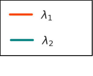
(b) To provide visual intuition for the behavior of adaptive variance mitigation, we report the values of and over the training duration in Figure 2. As several factors are combined through (12) to influence the values, it is hard to pinpoint any individual factor that is responsible for the observed trend. However, note that for both the routing problem in San Francisco and the robot navigation in maze, the goal reward is obtained on reaching the destination and intermediate actions do not impact the total return significantly. Intuitively, this makes the action set conditioned baseline similarly correlated to the observed return as the state only conditioned baseline, , but at the expense of estimating significantly more number of parameters. Thus the importance for is automatically adapted to be closer to zero. On the other hand, in recommender system, each product has a significant amount of associated reward. Therefore, the total return possible during each episode has a strong dependency on the available action set and thus the magnitude of weight for is much larger than that for .
(c) To understand the impact of the probability of an action being available, we report the best performances for all the algorithms for different probability values in Figure 3. We notice that in the San Francisco routing domain, SAS-Q-learning has a slight edge over the proposed methods. This can be attributed to the fact that off-policy samples can be re-used without causing any divergence problems as state features are not shared. For the maze and the recommender system tasks, where function approximators are necessary, the proposed methods significantly out-perform SAS-Q.
Conclusion
Building upon the SAS-MDP framework of ? (?), we studied an under-addressed problem of dealing with MDPs with stochastic action sets. We highlighted some of the limitations of the existing method and addressed them by generalizing policy gradient methods for SAS-MDPs. Additionally, we introduced a novel baseline and an adaptive variance reduction technique unique to this setting. Our approach has several benefits. Not only does it generalize the theoretical properties of standard policy gradient methods, but it is also practically efficient and simple to implement.
Acknowledgement
The research was supported by and partially conducted at Adobe Research. We are also immensely grateful to the three anonymous reviewers who shared their insights and feedback, specially to the second reviewer who helped improve the counter example.
References
- [2007] Amari, S.-i., and Nagaoka, H. 2007. Methods of information geometry, volume 191. American Mathematical Soc.
- [1998] Amari, S.-I. 1998. Natural gradient works efficiently in learning. Neural computation 10(2):251–276.
- [2003] Bagnell, J. A., and Schneider, J. G. 2003. Covariant policy search. In IJCAI-03, Proceedings of the Eighteenth International Joint Conference on Artificial Intelligence.
- [1995] Baird, L. 1995. Residual algorithms: Reinforcement learning with function approximation. In Machine Learning Proceedings 1995. Elsevier. 30–37.
- [2000] Bertsekas, D. P., and Tsitsiklis, J. N. 2000. Gradient convergence in gradient methods with errors. SIAM Journal on Optimization 10(3):627–642.
- [2008] Bhatnagar, S.; Ghavamzadeh, M.; Lee, M.; and Sutton, R. S. 2008. Incremental natural actor-critic algorithms. In Advances in neural information processing systems, 105–112.
- [2018] Boutilier, C.; Cohen, A.; Daniely, A.; Hassidim, A.; Mansour, Y.; Meshi, O.; Mladenov, M.; and Schuurmans, D. 2018. Planning and learning with stochastic action sets. In IJCAI.
- [2012] Degris, T.; Pilarski, P. M.; and Sutton, R. S. 2012. Model-free reinforcement learning with continuous action in practice. In Proceedings of the 2012 American Control Conference.
- [2000] Feng, Y., and Yan, H. 2000. Optimal production control in a discrete manufacturing system with unreliable machines and random demands. IEEE Transactions on Automatic Control.
- [2018] Geffner, T., and Domke, J. 2018. Using large ensembles of control variates for variational inference. In Advances in Neural Information Processing Systems.
- [1996] Gendreau, M.; Laporte, G.; and Séguin, R. 1996. Stochastic vehicle routing. European Journal of Operational Research.
- [1996] Gordon, G. J. 1996. Chattering in sarsa(lambda). A CMU Learning Lab Internal Report.
- [2017] Grathwohl, W.; Choi, D.; Wu, Y.; Roeder, G.; and Duvenaud, D. 2017. Backpropagation through the void: Optimizing control variates for black-box gradient estimation. arXiv preprint arXiv:1711.00123.
- [1959] Graybill, F. A., and Deal, R. 1959. Combining unbiased estimators. Biometrics 15(4):543–550.
- [2004] Greensmith, E.; Bartlett, P. L.; and Baxter, J. 2004. Variance reduction techniques for gradient estimates in reinforcement learning. Journal of Machine Learning Research 5(Nov):1471–1530.
- [2007] Harper, G. W., and Skiba, S. 2007. User-personalized media sampling, recommendation and purchasing system using real-time inventory database. US Patent 7,174,312.
- [2003] Kakade, S. M., et al. 2003. On the sample complexity of reinforcement learning. Ph.D. Dissertation, University of London London, England.
- [2002] Kakade, S. M. 2002. A natural policy gradient. In Advances in neural information processing systems, 1531–1538.
- [2009] Kanade, V.; McMahan, H. B.; and Bryan, B. 2009. Sleeping experts and bandits with stochastic action availability and adversarial rewards. In Proceedings of the Twelfth International Conference on Artificial Intelligence and Statistics, AISTATS.
- [2010] Kleinberg, R.; Niculescu-Mizil, A.; and Sharma, Y. 2010. Regret bounds for sleeping experts and bandits. Machine learning.
- [2011] Konidaris, G.; Osentoski, S.; and Thomas, P. 2011. Value function approximation in reinforcement learning using the fourier basis. In Twenty-fifth AAAI conference on artificial intelligence.
- [2017] Liu, H.; Feng, Y.; Mao, Y.; Zhou, D.; Peng, J.; and Liu, Q. 2017. Action-depedent control variates for policy optimization via stein’s identity. arXiv preprint arXiv:1710.11198.
- [2007] Mahdian, M.; Nazerzadeh, H.; and Saberi, A. 2007. Allocating online advertisement space with unreliable estimates. In Proceedings of the 8th ACM conference on Electronic commerce. ACM.
- [1994] Meir, R., et al. 1994. Bias, variance and the combination of estimators: The case of linear least squares. Citeseer.
- [2005] Morimura, T.; Uchibe, E.; and Doya, K. 2005. Utilizing the natural gradient in temporal difference reinforcement learning with eligibility traces. In International Symposium on Information Geometry and its Application, 256–263.
- [2008] Nikolova, E., and Karger, D. R. 2008. Route planning under uncertainty: The canadian traveller problem. In AAAI.
- [2006] Nikolova, E.; Brand, M.; and Karger, D. R. 2006. Optimal route planning under uncertainty. In ICAPS, volume 6, 131–141.
- [1991] Papadimitriou, C. H., and Yannakakis, M. 1991. Shortest paths without a map. Theoretical Computer Science 84(1):127–150.
- [1996] Polychronopoulos, G. H., and Tsitsiklis, J. N. 1996. Stochastic shortest path problems with recourse. Networks: An International Journal 27(2):133–143.
- [2008] Ribeiro, A.; Sidiropoulos, N. D.; and Giannakis, G. B. 2008. Optimal distributed stochastic routing algorithms for wireless multihop networks. IEEE Transactions on Wireless Communications.
- [2018] Sutton, R. S., and Barto, A. G. 2018. Reinforcement learning: An introduction. MIT press.
- [2000] Sutton, R. S.; McAllester, D. A.; Singh, S. P.; and Mansour, Y. 2000. Policy gradient methods for reinforcement learning with function approximation. In Advances in neural information processing systems, 1057–1063.
- [2012] Tan, B., and Srikant, R. 2012. Online advertisement, optimization and stochastic networks. IEEE Transactions on Automatic Control.
- [2015] Theocharous, G.; Thomas, P. S.; and Ghavamzadeh, M. 2015. Ad recommendation systems for life-time value optimization. In Proceedings of the 24th International Conference on World Wide Web, 1305–1310. ACM.
- [2012] Thomas, P. S., and Barto, A. G. 2012. Motor primitive discovery. In Procedings of the IEEE Conference on Development and Learning and Epigenetic Robotics, 1–8.
- [2017] Thomas, P. S., and Brunskill, E. 2017. Policy gradient methods for reinforcement learning with function approximation and action-dependent baselines. arXiv preprint arXiv:1706.06643.
- [2018] Thomas, P.; Dann, C.; and Brunskill, E. 2018. Decoupling gradient-like learning rules from representations. In International Conference on Machine Learning.
- [2014] Thomas, P. 2014. Bias in natural actor-critic algorithms. In International Conference on Machine Learning, 441–448.
- [1983] Tsitsiklis, J., and Roy, B. 1983. An analysis of temporal-difference with function approximation. IEEE Trans. Autom. Control 42(5):834–836.
- [2018] Tucker, G.; Bhupatiraju, S.; Gu, S.; Turner, R. E.; Ghahramani, Z.; and Levine, S. 2018. The mirage of action-dependent baselines in reinforcement learning. arXiv preprint arXiv:1802.10031.
- [2013] Wang, C.; Chen, X.; Smola, A. J.; and Xing, E. P. 2013. Variance reduction for stochastic gradient optimization. In Advances in Neural Information Processing Systems.
- [2018] Wu, C.; Rajeswaran, A.; Duan, Y.; Kumar, V.; Bayen, A. M.; Kakade, S.; Mordatch, I.; and Abbeel, P. 2018. Variance reduction for policy gradient with action-dependent factorized baselines. arXiv preprint arXiv:1803.07246.
Reinforcement Learning When All Actions are Not
Always Available (Supplementary Material)
Appendix A A: SAS Policy Gradient
Lemma 1 (SAS Policy Gradient).
For all ,
| (13) |
Proof.
| (14) | ||||
| (15) | ||||
| (16) | ||||
| (17) | ||||
| (18) | ||||
| (19) | ||||
| (20) |
where (19) comes from unrolling the Bellman equation. We started with the partial derivative of the value of a state, expanded the definition of the value of a state, and obtained an expression in terms of the partial derivative of the value of another state. Now, we again expand using the definition of the state-value function and the Bellman equation.
| (21) | ||||
| (22) | ||||
| (23) | ||||
| (24) |
| (25) | ||||
| (26) | ||||
| (27) | ||||
| (28) | ||||
| (29) | ||||
| (30) | ||||
| (31) | ||||
| (32) | ||||
| (33) |
Expanding allowed us to write it in terms of the partial derivative of yet another state, . We could continue this process, “unravelling” the recurrence further. Each time that we expand the partial derivative of the value of a state with respect to the parameters, we get another term. The first two terms that we have obtained are marked above. If we were to unravel the expression more times, by expanding and then differentiating, we would obtain the subsequent third, fourth, etc., terms.
Finally, to get the desired result, we expand the start-state objective and take the derivative with respect to it,
| (34) |
Combining results from (33) and (34), we index each term by , with the first term being , the second , etc., which results in the expression:
| (35) |
Notice that to get the gradient with respect to , we have included a sum over all the states weighted by, , the start state probability. When , the only state where is not zero will be when (at which point this probability is one). This allows us to succinctly represent all the terms. With this we conclude the proof. ∎
Appendix B B: Convergence
Lemma 2.
Appendix C C: SAS Natural Policy Gradient
Property 1 (Fisher Information Matrix).
For a policy, parameterized using weights , let , then the Fisher information matrix is,
| (36) |
Proof.
To prove this result, we first note the following relation by ? (?) which connects the Hessian and the FIM of a random variable parameterized using ,
| (37) |
Now, let denote the random variable corresponding to the trajectories observed using policy . Let denote an outcome of , then the probability of observing this trajectory, , is given by,
| (38) | ||||
| (39) |
Therefore,
| (40) | ||||
| (41) | ||||
| (42) |
We know that Fisher Information Matrix for a random variable, which in our case is , is given by,
| (43) | |||||
| (Using Equation (37)) | (44) | ||||
| (Using Equation (42)) | (45) | ||||
| (46) | |||||
where the summation over corresponds to all possible values of and for every step in the trajectory. Expanding the inner summation in (46),
| (47) |
Note that the summation in (47) over all possible trajectories, i.e. all possible values of and for every step , marginalizes out the terms not associated with respective terms, i.e.,
| (48) | ||||
| (49) | ||||
| (50) |
Combining all the terms in (50) and discounting them appropriately with , we get,
| (51) |
Finally, note that using (37),
| (52) |
Combining (51) and (52) we get,
| (53) |
With this we conclude the proof. ∎
Lemma 3 (SAS Natural Policy Gradient).
Let be a parameter such that,
| (54) |
then for all in ,
| (55) |
Appendix D D: Adaptive Variance Mitigation
Property 2 (Unbiased estimator).
Let and , then for any values of and ,
| (64) |
Proof.
Lemma 4 (Adaptive variance mitigation).
Let
| (74) | ||||
| (75) | ||||
| (76) |
such that, and , then the that minimizes variance of is given by,
| (77) |
Proof.
Let the sample estimate for the gradient be given by,
| (78) |
We aim to find the values of that minimizes the variance of this estimator, i.e.,
| (79) |
The variance of the estimator can be computed as following,
| (80) | ||||
| (81) | ||||
| (82) |
From Property 2 we know that,
| (83) | ||||
| (84) | ||||
| (85) |
Expanding (82) in the matrix notations,
| (86) | ||||
| (87) |
Since the first and last term from (87) are independent of , it does not effect the optimization step. The remaining terms that matter are,
| (88) |
Differentiating these terms with respect to , and by equating it to , we get,
| (89) | ||||
| (90) | ||||
| (91) | ||||
| (92) |
∎
Appendix E E: SAS Natural Policy Gradient
Pseudo-code for SAS natural policy gradient is provided in Algorithm 2. Let the learning-rate for updating and be given by and , respectively. Similar to Algorithm 1, we first collect the transition batch and compute the sampled returns from each state in Lines and . Following Lemma 3, we update the parameter in Line to minimize its associated TD error. The updated parameter is then used to update the policy parameters . As dividing by a scalar does not change the direction of the (natural) gradient, we normalize the update using norm of in Line for better stability.
# Perform batch update on parameters
Update
Update
Appendix F F: Empirical Analysis Details


Implementation details
Policy parmaterization.
To make the policy handle stochastic action sets, we make use of a mask which indicates the available actions. Formally, let be the feature vector of the state and let denote the parameters that project the features on the space of all actions. Let denote the scores for each action and let be the indicator variable denoting whether the action is in the available action set or not. The probability of choosing an action is then computed using the masked softmax, i.e.,
| (93) |
where corresponds to the score of action in .
Hyperparamter settings.
For the maze domain, state features were represented using order coupled Fourier basis [2011]. For the San Francisco map domain, one-hot encoding was used to represent each of the nodes (states) in the road-network. For the recommender system domain, the user-context provided by the environment was directly used as state-features. Using these features, single layer-neural networks were used to represent the policy, baselines and the q-function for all the algorithms, for all the domains. The discounting parameter was set to for all the domains.
For SAS policy gradient, the learning rates for both the baselines were searched over . The learning rate for policy was searched over . The hyper-parameter was kept fixed to throughout. For SAS natural policy gradient, the learning rate, , was searched over .
For SAS-Q-learning baseline, the exploration parameter for -greedy was searched over and the Learning rate for the q-function was searched over . To encompass both online and batch learning for SAS-Q-learning, additional hyperparameter search was done over the batch-sizes and the number of batches per update to the q-function. Note that when both the batch size and the number of batches is , it becomes the online version [2018].
In total, settings for each algorithm, for each domain, were uniformly sampled from the mentioned hyper-parameter ranges/sets. Results from the best performing setting is reported in all the plots. Each hyper-parameter setting was ran using different seeds to get the standard deviation of the performance.
Additional Experimental Results
In Figures 5 and 6 we report the learning curves and the adapted and values for all the domains under different probability values of action availability.


