On General Lattice Quantization Noise
Abstract
The problem of constructing lattices such that their quantization noise approaches a desired distribution is studied. It is shown that asymptotically in the dimension, lattice quantization noise can approach a broad family of distribution functions with independent and identically distributed components.
I Introduction
Lattices play a key role in digital communication and specifically in quantization theory. In high-resolution quantization theory, it is common to assume (see, e.g, [5] and references therein) that the quantization error of a lattice quantizer is uniformly distributed over the basic cell of the lattice. This assumption can be made completely accurate at any resolution by means of subtractive dithered quantization, where a random vector (dither) which is uniformly distributed over the lattice cell is added prior to quantization and then subtracted from the quantizer output (see [6]). Following [10] we thus use the term lattice quantization noise (LQN) to refer to a random vector uniformly distributed over a basic cell of the lattice. For a given lattice however there are many possible partitions into cells. Each such partition will result in a different LQN with different statistical properties (see [7]).
In many cases of interest, the criterion for quantization is that of minimum mean-square error (MSE). That is, a lattice is deemed good if the MSE of the quantization noise (resulting from nearest neighbor encoding) is minimal for a given lattice density (or cell volume). When the criterion is MSE, the basic region associated with nearest neighbor encoding (in the Euclidian sense) is called the Voronoi region. The statistical properties of LQN of lattices which are good in this sense has been thoroughly investigated by Zamir and Feder [10]. Indeed, it was shown in [10] that there exist sequences of lattices which are asymptotically optimal in an MSE sense. That is, for such sequences, the normalized second moment of the Voronoi region of the lattice goes to as the dimension goes to infinity and the distribution of quantization noise (over a Voronoi region) approaches (in the Kullback-Leibler divergence sense) that of an i.i.d. white Gaussian noise.
In certain cases, the criterion for quantization may be different from MSE. For instance one may be interested in some other metric, e.g., an -th power norm. More generally, one may ask whether one can construct a lattice and associate with it a lattice partition such that the corresponding LQN approaches any i.i.d. distribution. The interest of the authors in this question arose when general LQN was needed in the context of designing a lattice precoding scheme for the binary dirty paper problem [4].
The results of [10] were derived using previously known results [9] on the existence of lattices that are good for the classical problem of covering. This approach unfortunately does not lend itself to extending the results to more general distributions. On the other hand, typicality arguments and rate distortion theory suggest that a random code drawn uniformly over a large region should have the desired properties. Since linear codes and lattices have proved to be able to attain the performance of a (uniform) random code in many problems in information theory, it is natural to suspect that the same would hold for the problem at hand.
Indeed, one may use random coding (or averaging arguments) to obtain existence results for lattices, an approach dating back at least as far as Hlawka’s proof of the Minkowsk-Hlawka theorem, see [8] for an historical account and further details. In [8], Loeliger defined an ensemble of lattices based on Construction A (see [1]) which is very amenable to analysis. Loeliger then used averaging and typicality arguments to obtain channel coding theorems for lattice codes.
In [3] the Loeliger ensemble (with a careful choice of parameters) was used to establish the existence of lattices that are simultaneously good under various different notions. It was further noted in [3] that the results can be extended to show that there exist lattices that are good for quantization under any -th norm. In this work we extend these results to show that under quite general conditions, LQN can approach general i.i.d. distributions. In the proof we use the same ensemble of lattices as in [8] and [3]. However, the proof technique diverges from that of [3] in that it relies on typicality as in [8] rather than geometric arguments to form the lattice cells. In this sense the present work is dual to Loeliger’s work [8] , using typicality arguments to obtain results for source coding (rather than for channel coding as in [8]).
The paper is organized as follows. Section II provides a very brief introduction to lattices and lattice quantization noise as well as states the main result of the paper for both the discrete and continuous cases. Section III describes the ensemble of lattices to be used and defines the typicality-based lattice partition. Sections IV and V provides the proof for the existence of a lattices whose quantization noise approaches a desired distribution. Finally, the results are demonstrated in Section VI by simulation, finding lattices and partitions with quite arbitrary LQN noise.
II Preliminaries and statement of main result
II-A Lattices and Lattice Quantization Noise
We begin by recalling a few basic notions pertaining to lattices. An -dimensional lattice is an infinite discrete subgroup of the Euclidean space . Thus, if and are in , then their sum and difference are also in . An -dimensional lattice may be defined by an generating matrix (whose choice is not unique) such that
We may associate with a lattice a lattice partition, partitioning into disjoint cells. We denote by the fundamental cell associated with . We further associate with every lattice point the cell . There are many possible choices for . For to be valid however, we require that every point can be uniquely written as where is a lattice point and is the “remainder”. We may thus write . The lattice partition is therefore fully determined by the specification of the fundamental region . The volume of a fundamental region is the same for any valid partition and we denote it by or simply by .
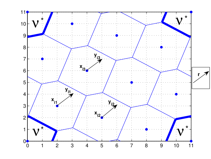
We note that when the partition is such that a point is mapped to the nearest lattice point in in the Euclidean sense, we obtain the usual Voronoi partition. An example of lattices and lattice partitions is given in Figure 1.

We further associate with a lattice and a chosen partition a lattice quantizer . For any , since it may be written as in one and only way, we define to be the quantization of . We further define a modulo operation by,
For any input vector , we may view the remainder as the “quantization noise” associated with . A random vector uniformly distributed over is referred to as (random) LQN.
II-B Statement of main result
Let be an i.i.d. random vector with marginal Probability Density Function (PDF) denoted by . Then we would like to find a sequence of lattices and corresponding partitions such that the associated LQN approaches an i.i.d. distribution with marginal PDF .
Definition 1
A random variable with a continuous PDF will be called permissible if is bounded from below by a positive number over a closed interval , and is zero outside of , i.e,
| (1) |
where is some arbitrarily small fixed value, and is some arbitrarily large fixed value.
Theorem 1
Let be a permissible noise with PDF . Let be drawn i.i.d. . Then, there exists a sequence of lattices and associated partitions such that the resulting lattice quantization noise satisfies,
| (2) |
where is the Kullback-Leibler divergence and can be taken arbitrarily small.
This theorem also results in the following corollary that shows convergence of the marginal PDFs to the desired one (in an average sense).
Corollary 1
Let be a permissible noise with PDF . Let be drawn i.i.d. . Then there exists a sequence of lattices and associated partitions such that the resulting lattice quantization noise, satisfies,
| (3) |
where can be taken arbitrarily small.
The key to proving this theorem lies in proving a similar claim for the discrete case which we state next. The proof for the continuous case follows from the discrete case by standard arguments, dividing the interval into small enough intervals and is given in Section V.
II-C Discrete case
We now restrict our attention to the discrete space . We begin by recalling some basic definitions which are analogous to those provided above for the continuous setting.
A fundamental cell associated with the lattice is a finite set such that any point can be written in one and only one way as where and . We further define the corresponding quantizer and LQN as before.
Let be a prime number. The following notation will be used in the paper to denote componentwise modulo operations:
- •
For any scalar random variable , .
- •
For any vector random variable , is the result of reducing each component of modulo .
The discrete counterparts of Definition 1, Theorem 1, and Corollary 1 are:
Definition 2
A random variable with a discrete probability function will be called -permissible if takes values in and is a strictly positive probability function, i.e.,
where (with abuse of notation) is some arbitrarily small fixed value.
Theorem 2
Let be a -permissible noise with a PDF where is a prime number. Let be drawn i.i.d. . Then, there exists a sequence of integer valued lattices and associated partitions such that the resulting lattice quantization noise, , satisfies,
| (4) |
Corollary 2
Let be a -permissible noise with a PDF where is a prime number. Let be drawn i.i.d. . Then there exists a sequence of lattices and associated lattice partitions such that the resulting lattice quantization noise, , satisfies
| (5) |
III Ensemble of Lattices and Lattice Partition
We make use of the Loeliger ensemble of lattices [8] based on Construction A (see [1]). Let , , be integers such that and let be a prime number. Let be a generating matrix with elements in . Then a lattice may be obtained from using Construction A as depicted in Figure 2. The construction consists of the following steps:
- •
Define the codebook , where all the operations are modulo-. Thus . The rate of the code11 1 All logarithms in this paper are taken to base . (in bits per sample), , is defined by
(6) - •
Replicate over to form the lattice . It is easy to show that is indeed a lattice, see, e.g., [1].
The random ensemble of lattices is generated by drawing each entry of the generating matrix according to a uniform i.i.d. distribution over , resulting in a random codebook22 2 We note that with this notation (numbering), some of the codewords may be identical (when is not full rank). That is of no consequence to the analysis. , and applying the steps described above.
We note that Construction A results in a lattice that is periodic with respect to the lattice as can be seen in Figure 2. Thus, when analyzing the properties of the lattice, one may restrict attention to the the basic cube (the region highlighted in Figure 2), i.e., to the region . In particular, for any lattice and fundamental region , we define the “folded” fundamental region as depicted in Figure 3. It is easy to see that plays the same role with respect to the code as does with respect to . That is, for each one may write where and . Note also that in the same manner that specifying induces the folded region , the converse is also true. Specifying the region with respect to the code , naturally induces the region with respect to the lattice. Further, let be a vector in . We observe that (where the first modulo operation is performed with respect to ) is equal to (where the modulo operation is performed with respect to ). That is, the order of the modulo operations can be exchanged. We conclude that for a lattice obtained by Construction A, defining is equivalent to defining . We may therefore focus on the latter task.

We introduce now the technique by which we partition for a given lattice and target PDF . We rely on typicality (see, e.g., [2]) and use the following notation:
- •
: The set of vectors in that are -typical to .
- •
: The set of all pairs of vectors in such that their difference modulo is -typical to the PDF of .
We go over all points . For any not yet associated to a cell we associate it according to the following two possibilities:
- 1.
There is no such that : We arbitrarily associate to and .
- 2.
There exists at least one codeword such that : We choose one such codeword and add to .
For any such vector , we also associate all the “coset members” to the their respective cells . Thus, in each step we first associate the vector to the basic cell and then map the coset members. We then apply the procedure again until all vectors have been associated. This procedure is depicted in Figure 3.
IV Proof of Theorem 2
We now show that indeed we obtain an ensemble of lattices and associated partitions such that the LQN has the desired properties, for almost all members of the ensemble. The main steps are as follows. Lemma 1 shows that for any vector in the probability to find a codeword such that their difference (modulo ) is typical to goes to one as the dimension goes to infinity, with a proper choice for the rate of the codebooks. We conclude that there exists a specific sequence of codebooks that can match almost every point of and then show that such a sequence yields the desired LQN. In the sequel we form the partitioning letting decrease with dimension as:
| (7) |
Any other vanishing function of would be appropriate.
IV-A Almost all points are matchable
For every code , let be a randomly shifted version of the codebook (i.e., is a random coset code) where is a random vector uniformly distributed over . We denote the codewords of by , . Thus, .
For a given , we call the event in which there is no codeword in such that its difference from modulo is typical to , as a “bad event”. Defining the indicator random variable,
a bad event amounts to the event . The next lemma shows that with a proper choice of code rate, such “bad events” are rare.
Lemma 1
Let be a linear codebook of rate drawn from the random ensemble defined above and let be the induced random coset code. Let be any given vector. Then, for a rate satisfying
| (9) |
we have
| (10) |
where the probability is averaged over all codebooks and over all shifting random vectors, and as defined in (7).
The proof is given in Appendix A.
Denote by the number of vectors that can be matched. We note that
where the expectation is over all codebooks and all shifting random vectors. By Lemma 1, taking to infinity we get
Note that this result applies also to the original (non-shifted) ensemble (and for any other constant-shifted ensemble) due to symmetry. Thus, for any shift vector , where the expectation on the r.h.s is only over the lattice ensemble.
An immediate consequence is that there exists a specific sequence of codebooks for which
| (11) |
We focus our attention on such a sequence and consider the corresponding sequence of fundamental regions. Let us denote the set of matchable sequences in by and the non-matchable by . From the symmetrical construction of the cells and from (11) it follows that:
| (12) |
Thus almost all points in are typical to .
IV-B Convergence in divergence
We now show that the resulting LQN reduced modulo , , asymptotically approaches the desired distribution. The construction suggested above creates cells, each with elements. Thus, assumes one of values with equal probability. We now relate the entropy of to the volume of a cell. We take the rate of the code to satisfy (9) with equality, i.e.,
| (13) |
where is defined in (7). We thus have
or equivalently
We observe that
- •
For each ,
(14) - •
- •
For , . Defining
(16) it follows that
(17) for any .
We thus have,
Dividing both sides by , we get
| (18) | |||||
| (19) |
where
| (20) |
From (12) it follows that the second term of the r.h.s. of (20) vanishes as goes to infinity. In addition, it is clear (by its definition) that vanishes as well as goes to infinity and hence the same applies to . This completes the proof of Theorem 2.
V Tying it all together
We turn to proving Theorem 1. We show how we may generate any desired continuous distribution, subject to mild regularity conditions, by building on the results derived for the discrete case. Let us denote the desired permissible continuous LQN by and its PDF by . First, divide into small enough -size intervals, where will be a constant value such that
| (21) |
is a prime number. The larger the value of , the more refined the approximation for will be. We then use the following steps to construct the lattice and lattice partition:
- •
Define the folded random variable by,
(22) - •
Define the quantized random variable by,
(23) where takes values in . Denote the PDF of by .
- •
Generate the sequence of lattices and lattice partitions, , as described in the previous section such that the associated LQN approaches an i.i.d. distribution with marginal PDF .
- •
Scale the lattice by , i.e
(24) - •
Define the continuous fundamental region, , by,
(25) where
(26) That is, we scale by a factor of and add a -size cube to each element.
These steps are exemplified in Figures 4 and 5. Figure 4 depicts a discrete lattice with where the codewords are designated with ‘x‘. The cell of some codeword is designated with dots. Figure 5 depicts the equivalent continuous lattice with . Here the codewords are designated with ‘x‘ while the cells are drawn with a solid line.
Let be the resulting LQN. In Appendix B we show that indeed the construction yields an LQN which PDF that can approximate to any desired degree in a Kulback-Leibler divergence sense, thus completing the proof of Theorem 1.


VI Simulation Results
In this section we demonstrate the theoretical results via simulation. Since for complexity reasons we are limited to using only small dimensions, we replaced the typicality criterion with the maximum likelihood criterion. In addition, instead of choosing a lattice at random, we generated at random codebooks and picked the codebook that maximizes .
We considered the following cases:
- •
,
- •
,
- •
,
- •
, as depicted in Figure 10.
Figure 6 shows the lattice partition that was obtained for the “step like” distribution . The codewords are designated with ‘x‘. The cell of some codeword is designated with dots. As expected, the lattice cell has a shape of a square and the divergence from the desired distribution is .

Figure 7 shows the lattice partition obtained for .

Figures 8 and 9 refer to the distribution of the third case. Figure 8 depicts the relative entropy corresponding to each value of the rate (corresponding to ). The optimal value was obtained for the rate that was the closest to as should be expected.

Figure 9 depicts the marginal distribution of each element of the vector that was obtained using the optimal rate, which is in good agreement with .

Finally, Figure 10 depicts the desired PDF . The simulation was run for dimension and with (for this is the optimal value for ). Figure 11 depicts the marginal distribution of the obtained LQN which is in good agreement with the desired one.


VII Summary
It was demonstrated that subject to mild regularity conditions, lattice quantization noise may approach (asymptotically in the dimension) quite general distributions, with a proper choice of lattice and partitioning.
VIII APPENDIX
A Proof Of Lemma 1
We note that by standard arguments the codewords of are pairwise independent and uniformly distributed over . Define the indicator random variables
and note that they are also pairwise independent. We have
and
where
Note that is independent of the vector . Since plays no role in the analysis, we thus omit it from the notation and use below.
We note that is drawn uniformly over . Therefore, the difference is also distributed uniformly over . Thus,
where the inequality follows from the definition of typicality (i.e., by Theorem 3.1.2 in [2]).
We denote by the total number of codewords in and bound the probability of a “bad event” (no match) by
| (29) | |||||
where the fourth transition is due to Chebyshev’s inequality using the fact that . Thus, for any , as goes to infinity.
B Proof Of Continuous Case
In this Appendix we show that the construction of lattices and lattice partitions as has been described in Section V allows us to approach the desired distribution as closed as desired.
We note that each can be uniquely written as where and . For every we denote the unique associated with it by .
Consider the random vector defined in (23). That is, each component is the quantization of . We further note that
| (30) | |||||
Let be the “folded” continuous fundamental region and let be the “folded” LQN. Note that . Define the quantized random variable by,
| (31) |
where takes values in and consider the random vector where each component is the quantization of . Note that
| (32) |
Define by:
| (33) | |||||
| (34) |
where
| (35) |
and where
| (36) |
and
We observe that
- •
- •
- •
Using the sequence of lattices proposed in Theorem 2 we obtain,
| (38) | |||||
Dividing both sides by , we get
| (39) |
where is defined in (19). Therefore,
| (40) | |||||
It remains to choose such that is close enough to . Note that since is permissible, it is continuous and limited to the closed interval . Therefore, is uniformly continuous, i.e, for any exists such that for any satisfying , it follows that . Therefore, can be lower bounded by
| (41) |
where is defined in (1). If we choose
| (42) |
and set , then and by (40),
| (43) |
C Proof Of Corollary
We prove Corollary 2 for the discrete case.
Proof:
We first use the chain rule for relative entropy (see Theorem 2.5.3 in [2]):
| (44) | |||||
Using Theorem 2.7.2 in [2] we get
| (45) | |||||
where the last transition is due to the fact that the elements of are i.i.d. Using (45) we get
Finally, we conclude that using the same sequence of lattices proposed in Theorem 2 results in
| (46) |
∎
References
- [1] J. H. Conway and N. J. A. Sloane, Sphere Packings, Lattices and Groups, volume 290 of Grundlehren der Matematischen Wissenschaften. Springer-Verlag, third edition, New York, 1998.
- [2] T. M. Cover and J. A. Thomas, Elements of Information Theory. Wiley, New York, 1991.
- [3] U. Erez, S. Litsyn and R. Zamir, Lattices Which Are Good for (Almost) Everything. IEEE Trans. Information Theory. IT-51, pp. 3401–3416, October 2005.
- [4] T. Gariby, U. Erez, S. Shamai. Dirty Paper Coding for PAM Signaling. In Proceedings of ISIT 2007, June 24-29, Nice, France.
- [5] R. M. Gray and D. L. Neuhoff, Quantization. IEEE Trans. Information Theory. IT-44, pp. 2325–2383, Oct. 1998.
- [6] R. M. Gray and JR.T. J. Stockham, Dithered Quantizers. IEEE Trans. Information Theory. IT-39, pp. 805–812, May 1993.
- [7] D. H. Lee and D. L. Neuhoff, Asymptotic distribution of the errors in scalar and vector quantizers. IEEE Trans. Information Theory. IT-42, pp. 446–460, March 1996.
- [8] H. A. Loeliger, Averaging bounds for lattices and linear codes. IEEE Trans. Information Theory. IT-43, pp. 1767–1773, November 1997.
- [9] C. A. Rogers, Packing and Covering. Cambridge, U.K.: Cambridge Univ. Press, 1964.
- [10] R. Zamir and M. Feder, On lattice quantization noise. IEEE Trans. Information Theory. IT-42, pp. 1152–1159, July 1996.