Prospects for Detecting X-ray Polarization in Blazar JetsFacilities: Swift, RXTE, RoboPol, Steward Observatory
Abstract
X-ray polarization should provide new probes of magnetic field geometry and acceleration physics near the base of blazar jets, but near-future missions will have limited sensitivity. We thus use existing lower energy data and X-ray variability measurements in the context of a basic synchro-Compton model to predict the X-ray polarization level and the probability of detection success for individual sources, listing the most attractive candidates for an IXPE campaign. We find that, as expected, several high-peak blazars such as Mrk 421 can be easily measured in 100 ks exposures. Most low peak sources should only be accessible to triggered campaigns during bright flares. Surprisingly, a few intermediate peak sources can have anomalously high X-ray polarization and thus are attractive targets.
Keywords:
relativistic processes - galaxies: active - galaxies: jetsI Introduction
The characteristic two peaked spectral energy distribution (SED) of blazar jet emission is understood to consist of a low energy synchrotron peak and a high energy maximum generally attributed to Compton emission, although in some models models hadronic processes may also contribute to the high energy flux (Boettcher 2012). Blazars are often classified by the synchrotron peak frequency , with Low-peak LSP reaching maxima in the mm-IR bands, Intermediate ISP sources peaking in the optical/UV and HSP peaking in the X-rays. Dramatic variability, on timescales down to minutes in a few cases (Ackermann et al. 2016), is another hallmark of blazar emission. While radiation-zone models can reproduce this general emission pattern, many details remain to be explained and the underlying mechanisms of jet energization and collimation are still a subject of debate (Blandford et al. 2018).
Polarization can be an important tool for probing the physics of the acceleration zone, especially in characterizing the magnetic field structures that control the expected shocks and induce synchrotron radiation. VLBI polarization maps have long been effective at measuring jet fields at pc-scale (e.g., Hovatta et al. 2012) while more recently optical polarization has provided new information on the field orientation and variability in the unresolved core (Blinov et al. 2018). X-ray polarization, to be measured by the approved Imaging X-ray Polarimetry Explorer (IXPE, Weisskopf 2018, launch 2021) and Enhanced X-ray Timing and Polarization mission (eXTP, Zhang et al. 2016, launch 2025), offers new opportunities to probe the jet fields and radiation physics, even closer to the acceleration site. In particular, polarization can help answer whether leptonic or hadronic process dominate in a given band (e.g., Zhang 2017).
However, the sensitivities of the near-future missions are modest and long exposures will be required, so in light of the variability and limited low energy polarization information one must choose the expected targets with care. We explore such choice here based on a simple synchro-Compton model. In section II we characterize the X-ray variability of sources observed in optical polarization monitoring programs, in section III we use our model to predict X-ray polarization levels (), while in section IV we combine these factors to quantify the success probability of an IXPE measurement for reasonable exposure in an untriggered observation, identifying a list of prime targets, and suggesting other X-ray bright sources that can also be of interest if they exhibit strong optical polarization. We conclude by discussing new measurements that can improve these predictions and monitoring campaigns that could make additional sources, and additional classes of polarization behavior, accessible in the X-ray band.
II X-ray variability
Since X-ray polarization measurements are in general sensitivity limited, source flux variability plays a key role in the prospects for a secure, 99% confidence, measurements of a given expected polarization level. We must therefore characterize the variability of likely targets, the great majority of which turn out to be sources detected by the Fermi LAT (Acero et al. 2015). We use 2-10 keV flux measurements from 2005-2017 measured by the Neil Gehrels Swift Observatory’s (hereafter Swift) LAT source monitoring program11 1 https://www.swift.psu.edu/monitoring/ (Stroh & Falcone 2013) supplemented by 2-10 keV fluxes (from 1995-2012) from the RXTE AGN timing and spectral database22 2 We have included all sources in the RXTE database classified as either BL Lac object (BL Lac) or Flat Spectrum Radio Quasar (FSRQ) with at least 20 observations. https://cass.ucsd.edu/rxteagn/ (Rivers et al. 2013). Stroh & Falcone 2013 analyze the individual Swift observations; we employ their mean spectral parameters tabulated for each source to convert epoch count rates to (2-10 keV) using WebPIMMS. 35 sources (19 LSPs, 2 ISPs, 13 HSPs and one unclassified source33 3 SED classification from the 3rd Fermi AGN catalog Acero et al. 2015, https://www.ssdc.asi.it/fermi3lac/) have at least 20 observations so that we can attempt a detailed variability analysis. For the remainder, we characterize their flux variability with a simple mean and standard variation.
Blazar high energy variability has been modeled as a log-normal distribution (e.g., Romoli et al. 2018; Shah et al. 2018), which may reflect disk-driven fluctuations (Lyubarskii 1997) or variations in the jet particle acceleration (Sinha et al. 2018). This suffices for some of our sources, but others show wider variability. This may indicate multiple jet states (e.g. quiescent and active flaring episodes), which can be represented by a double normal (Gaussian mixture) model (in log-space) (Liodakis et al. 2017). Of course if we have not sampled the full range of a source’s variability the two log-normals might be subsets of a broader single log-normal. Here, using the historical fluxes, we represent our flux distribution functions as either single or double log-normal models without attaching physical significance to the single or double-mode behavior.
The likelihood function for the single Gaussian model is defined as
| (1) |
where and are mean and standard deviation of the underlying distribution and and are the observed fluxes and their uncertainties (in log-space). For the Gaussian mixture the likelihood is defined as
| (2) | |||||
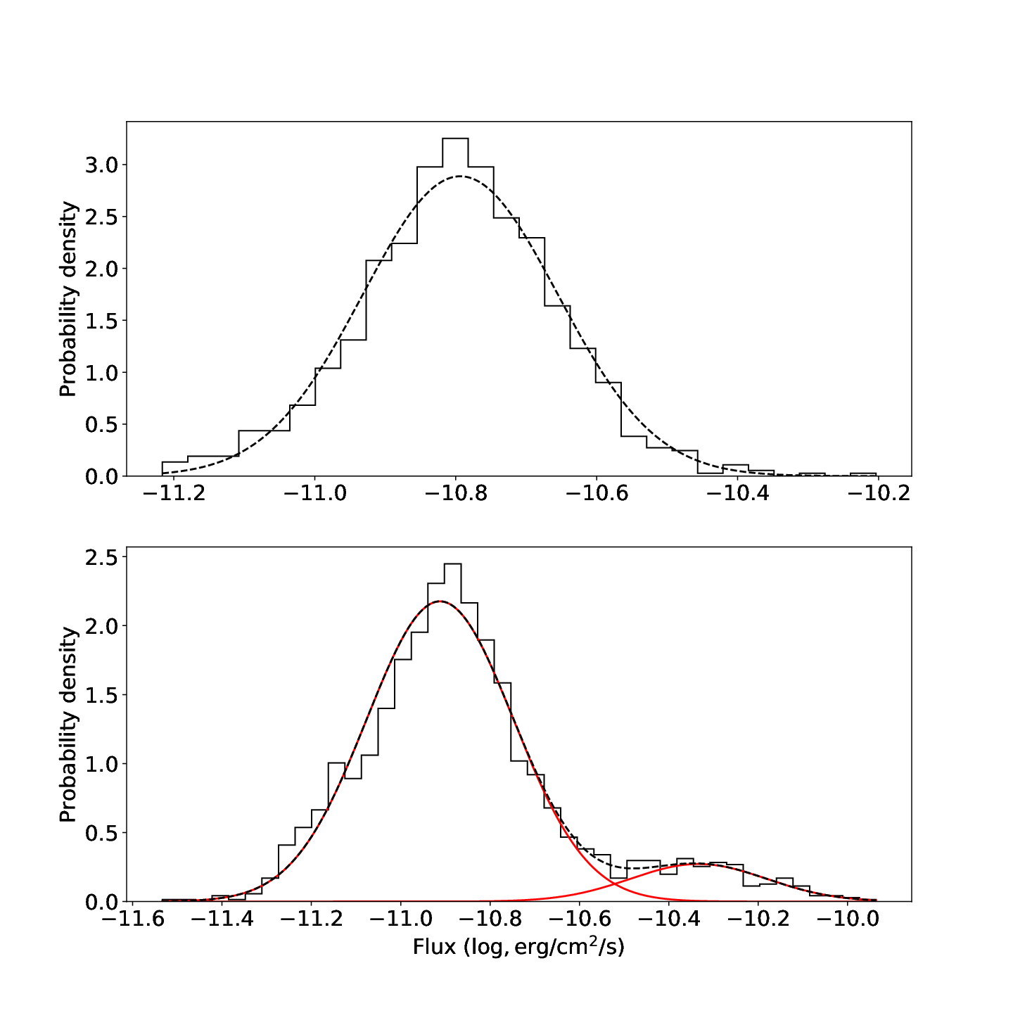
where we add mean and standard deviation and for a brighter ‘active’ state which is realized a fraction of the observed samples. With such a model, we can draw an arbitrary number of samples from the modeled distribution. To chose between models for a given source we use the Bayesian Information criterion (BIC). Figure 1 shows examples of best-fit models for PKS 0558-504 (top panel) and BL Lacertae (bottom panel). There are 15 sources best described as unimodal, 20 sources prefer a bimodal distribution. LSPs show no preference while HSPs slightly more commonly match a bimodal distribution (8 versus 5). The parameters of the best-fit distributions for all the sources are given in Table 1. For sources with observations, we simply record the mean and variance of the log of the flux, which can be used to form a log-normal distribution.
Measurements are easiest for high polarization sources in bright large states. Since both quantities are highly variable, we should test if they correlate, as might be expected from e.g. shock-driven flares (e.g., Marscher et al. 2008). Of course we lack , so we use the optical polarization () from the Robopol and Steward observatory monitoring programs which have significant temporal overlap with the Swift data for 17 sources. We use optical polarization as a tracer of the energetic electrons at the jet base that may also contribute X-ray synchrotron; radio polarization can be dominated by downstream emission. While we cannot make meaningful statements about individual sources, we can check the major source classes by stacking all contemporaneous observations from, say, the HSP. We find that both the LSP and HSP have a mild positive correlation (Spearman’s , significance ). The two ISP showed no correlation. Thus for LSPs and HSPs we draw a flux at a given level in their cumulative distribution function (CDF, e.g. a flux in the top X%) and then draw from that source’s polarization CDF at the same top X% level. For the ISP we will assume random uncorrelated draws (see §IV.1). In practice, we find that this makes a small % difference to the source detectability, so this assumption is not critical. However it should be tested with future monitoring campaigns.
III Expected
We must use the lower energy (optical) polarization degree to predict the polarization in the X-ray band. For the HSP and some ISP, the X-rays come from the same (synchrotron) component, while for the LSP and many ISP, they come from the low energy end of the high energy (here assumed to be Compton) peak. Particularly interesting are the ISP for which the synchro-Compton transition occurs within the IXPE band. To quantify this connection, we adopt a multizone jet picture (Peirson & Romani 2018), where the observed modest are the result of incoherent averaging of effective emission zones, each of which radiates with the expected for a uniform field, for a power-law population of electrons with index , producing the observed synchrotron spectrum. From observed polarization levels we typically infer for the emission cone contributing to the Earth line-of-sight. In practice, the zones have different angles to the line-of-sight and different characteristic particle energies so the number of zones, and thus , becomes a function of the observation frequency (e.g. Marscher & Jorstad 2010; Marscher 2014, Peirson & Romani 2019, ApJ in prep., hereafter PR2019).
This multizone picture, with distributions in and B field orientation, generally improves the match to observed blazar SEDs over that of a single-zone model. It also means that the for the individual zones vary and so the number of zones contributing half of the integrated flux is a function of frequency. A computation with related to the peak of the integrated spectrum, assuming typical jet beaming parameters, and a uniform squared distribution of randomly distributed among the zones is shown in the inset of Figure 2. The consequence is , with a small increase from the incoherently averaged half of the flux from the remaining zones (see PR2019 for details). Thus lets us relate the polarization at different frequencies across the synchrotron component. Note that the decrease and increase can be dramatic for ; some ISPs can be in this regime.
The behavior in Figure 2, where the range is more important than the effective Doppler factor variation, is slightly conservative. In some models, such as the shock model of Marscher 2014, may depend on the angle of to a shock front and hence to the jet axis; this organized variation further decreases when one is well above the synchrotron peak. We find that this effect is only important for , but there the polarization increase can be as much as an additional ; a few ISPs may have synchrotron X-rays from this extreme regime.

For HSP we can directly convert the optical band polarization level to the X-ray band using the square root of the ratios of the . We truncate at since our statistical estimate breaks down anyway. For some ISP, the increase can be substantial as long as the Compton component contributes weakly at 1-10 keV. For ISPs, we used the Space Science Data Center (SSDC) tools44 4 https://tools.ssdc.asi.it/SED/ to construct the SED of each source and determine whether the X-ray emission is synchrotron dominated. If so, we expect a substantial increase compared to the optical.
For LSP (and ISP with hard X-ray spectra) our model assumes that we observe Compton X-ray flux. This will only show polarization if the seed photon population is highly polarized (e.g., synchrotron emission). PR2019 find that for isotropic, many-zone scatting in typical jet geometries the resulting Compton polarization is that of the seed photons. This does depend on the viewing angle, opening angle, and Lorentz factor of the jet (see PR2019 for details). However for the typical jet parameters assumed in the present work (Liodakis et al. 2018) the retained polarization is near maximal, so we will assume . To get the latter, we scale from using Fig. 2. For X-ray Compton emission typical seed photons are in the mm-band, we will assume here GHz, but the dependence on the weighted effective seed photon frequency is weak. Note that we are assuming that all seed photons are synchrotron. If external photons contribute to the seed photon population will be lower. This means that our estimates of the LSP polarization may be optimistic. This is useful since any observed LSP polarization higher than our estimate indicates that the emission should be non-Compton in nature (e.g., proton synchrotron).
IV Blazar Detectability

Our prime target candidates are the sources measured with the RoboPol program55 5 http://robopol.org/ (Pavlidou et al. 2014; Blinov et al. 2018) and the Steward observatory66 6 http://james.as.arizona.edu/psmith/Fermi/ (Smith et al. 2009). For some of these we have Swift and/or RXTE monitoring, and so can construct a detailed variability model (§II). For the remainder we collect typical fluxes from the HEARSAC77 7 https://heasarc.gsfc.nasa.gov/ database. There are 103 sources with known SED class and at least one measurement in optical polarization and X-ray flux.
Armed with estimates of the X-ray flux and polarization and their variability we can make predictions for detectability. We focus on IXPE as the most imminent facility, whose sensitivity is estimated using the dedicated online tools88 8 https://ixpe.msfc.nasa.gov/cgi-aft/w3pimms/w3pimms.pl (Soffitta 2017; O’Dell et al. 2018). Typical exposures will be ksec, although the longest may approach a Msec. Figure 3 shows the X-ray flux and predicted X-ray polarization degree using the median and 1 confidence intervals from the PDFs for each source. These PDFs are estimated following §III. Note that with our assumed correlated fluctuations, HSP and LSP will vary diagonally (UR to LL) within these error bands. As expected, several HSPs are detectable at 100 ksec while a few (e.g., Mrk 421) might give significant measurements in 10 ksec, allowing a detailed variability study. Only few LSP sources are detectable, even with Msec exposures, under typical conditions. A few (e.g., 3C 454.3) are occasionally accessible in shorter time when bright and highly polarized.
IV.1 Detectability Duty Cycle
We must consider the substantial flux (§II) and polarization variability (e.g., Angelakis et al. 2016; Kiehlmann et al. 2017) when predicting the success of an X-ray polarization search. The uncertainty ranges in Figure 3 already give some idea of these effects. But some sources vary well outside these ranges, especially in occasional large flares and less often in polarization increases. Thus we use distribution function models to characterize the full variability range. For the X-ray variability we either use the parameters in Table 1 to construct a flux distribution function or use the mean and standard deviation to define a single log-normal model (see §II). For the optical polarization, we use distribution functions from the maximum likelihood modeling results of Angelakis et al. 2016 for RoboPol sources; for Steward Observatory-monitored sources we use their empirical CDF (Smith et al. 2009). As noted above for the ISPs we draw randomly for the CDFs, while for LSPs and HSPs we draw an and then adopt from the same probability level. We consider only sources with at least three observations in both optical polarization and X-ray flux and estimate the joint detection probability (DP) by computing the in a given exposure time and comparing with the predicted . We consider a simulated observation as a detection if . By repeating this calculation times we estimate the fraction of trials a source was detected. Dropping the flux- correlations results in decrease in the LSP, HSP detectability estimates. For the RXTE and Swift monitored sources we use the average spectral parameters and WebPIMMS to estimate the from the drawn flux value. For the remaining sources we use a photon index of 1.5 for inverse Compton and 2.5 for synchrotron emitting sources. In any case, assuming different spectral parameters results in only change in DP. Table 3 gives these detection probability values for an assumed 100 ksec IXPE exposure. They can be interpreted as the chance of success for a random observation at this exposure, or as the duty cycle for a triggered (by e.g., flux and/or monitoring) campaign. Of course, if one wants to measure a particular source, one can obtain more acceptable detection odds by increasing the exposure duration. While several HSPs have reasonable detection probabilities, only one ISP (CGRaBs J0211+1051) and one LSP (3C 454.3) are detected at 10% duty cycle. Thus long monitoring campaigns to allow bright trigger thresholds and/or longer IXPE exposures will be needed to reliably detect these source classes. It should be noted that source can vary by over a few days so longer exposures are not strictly ‘snapshots’ as computed here. Intraday variability is seen, but is uncommon enough to leave our 1 day detectability estimates unaffected.
IV.2 Sources without measured optical polarization
While many of the best and brightest candidates have been observed in existing optical polarization campaigns, there are other blazars that might be of interest. For example we find 208 blazars from the BZ catalog (Massaro et al. 2015) present in the Swift master catalog, 97 of which have and a known spectral class, so that we can evaluate their observability as a function of the unknown optical polarization level. With the observed X-ray flux we estimate the (accounting for the different source spectra as in section IV.1) as a function of exposure time. We convert this to expected optical polarization using the relation in Fig. 2. Figure 4 and Table 4 show the best prospects from this exercise. Table 4 also lists the minimum optical polarization that we would require for 100 ksec IXPE detections. This suggests that several more HSP and a few ISP are accessible in reasonable exposures, although one should obtain reconnaissance measurements first.

V Summary
We have used the archival SEDs of bright blazars along with observed optical polarization levels, to predict the expected 1-10 keV X-ray polarization in a basic synchro-self Compton model. This estimate, together with the historical X-ray flux level lets us evaluate the detectability of X-ray polarization for a given mission sensitivity. Including the flux and polarization variability as estimated by cumulative distribution functions modeled from historical data, lets us assess the probability that an exposure of given duration will achieve success. Equivalently, this gives the duty cycle for observations triggered by a monitoring campaign to be successful at a given exposure level. We compute these values for the characteristic IXPE mission sensitivity, giving a list of top candidate sources, useful for planning an observing campaign.
Unsurprisingly, HSP dominate the easily detectable sources, but a few ISPs with X-ray emission well above the synchrotron peak are surprisingly observable. In contrast few LSP can be accessed, and then only with long exposures. Recalling that our LSP estimate assumes correlated variability, and that no external seed photon flux dominates the up-scatter to the X-ray band, these LSP predictions should be considered optimistic for a Synchro-Compton model. However, other emission scenarios (e.g. proton synchrotron) for the high energy component can produce large , so a few LSP observations, especially when hadronic emission is indicated, would be desirable.
While our evaluation includes many of the brightest blazars, we have also identified a set which may be interesting targets, if the typical polarization level is sufficiently large. Optical reconnaissance to measure these and evaluate as possible targets for IXPE and/or eXTP are strongly encouraged.
| Name | Alt. name | SED | f | ||||
|---|---|---|---|---|---|---|---|
| J0152+0147 | 1RXS J015240.2+01 | HSP | - | -11.19 | 0.11 | - | - |
| J0210-5101 | PKS 0208-512 | LSP | 0.91 | -11.76 | 0.12 | -11.27 | 0.08 |
| J0222+4302 | 3C 66A | HSP | - | -11.16 | 0.06 | - | - |
| J0232+2017 | 1ES 0229+200 | HSP | 0.17 | -10.89 | 0.08 | -10.64 | 0.08 |
| J0238+1636 | PKS 0235+164 | LSP | 0.47 | -11.84 | 0.09 | -11.46 | 0.27 |
| J0324+3410 | 1H 0323+342 | HSP | - | -10.85 | 0.14 | - | - |
| J0530+1331 | PKS 0528+134 | LSP | - | -11.44 | 0.24 | - | - |
| J0539-2839 | PKS 0537-286 | LSP | - | -11.39 | 0.11 | - | - |
| J0559-5026 | PKS 0558-504 | - | - | -10.79 | 0.14 | - | - |
| J0721+7120 | S5 0716+714 | ISP | 0.16 | -11.1 | 0.35 | -10.21 | 0.15 |
| J0831+0429 | PKS 0829+046 | LSP | - | -11.46 | 0.08 | - | - |
| J0830+2410 | QSO B0827+243 | LSP | 0.79 | -11.70 | 0.13 | -11.08 | 0.12 |
| J0841+7053 | 4C 71.07 | LSP | - | -10.82 | 0.09 | - | - |
| J0854+2006 | OJ 287 | LSP | - | -11.37 | 0.18 | - | - |
| J1103-2329 | 1ES 1101-232 | HSP | 0.2 | -10.57 | 0.06 | -10.25 | 0.02 |
| J1104+3812 | Mrk 421 | HSP | 0.44 | -9.52 | 0.46 | -8.94 | 0.28 |
| J1159+2914 | 4C 29.45 | LSP | 0.23 | -11.46 | 0.09 | -11.08 | 0.03 |
| J1221+2813 | W Com | ISP | 0.73 | -12.07 | 0.06 | -11.80 | 0.22 |
| J1229+0203 | 3C 273 | LSP | 0.09 | -9.9 | 0.13 | -9.89 | 0.02 |
| J1256-0547 | 3C 279 | LSP | 0.83 | -11.24 | 0.09 | -10.94 | 0.21 |
| J1408-0752 | 1Jy 1406-076 | LSP | - | -12.25 | 0.09 | - | - |
| J1428+4240 | 1H 1430+423 | HSP | 0.52 | -10.64 | 0.2 | -10.08 | 0.12 |
| J1512-0905 | PKS 1510-089 | LSP | - | -11.07 | 0.13 | - | - |
| J1555+1111 | PG 1553+113 | HSP | 0.41 | -10.89 | 0.04 | -10.65 | 0.07 |
| J1626-2951 | PKS 1622-297 | LSP | 0.55 | -11.52 | 0.14 | -10.96 | 0.11 |
| J1635+3808 | 1Jy 1633+38 | LSP | - | -11.46 | 0.24 | - | - |
| J1653+3945 | Mrk 501 | HSP | - | -9.66 | 0.24 | - | - |
| J1733-1304 | NRAO 530 | LSP | - | -11.45 | 0.11 | - | - |
| J1959+6508 | 1ES 1959+650 | HSP | 0.79 | -9.93 | 0.22 | -9.27 | 0.25 |
| J2009-4849 | PKS 2005-489 | HSP | 0.51 | -11.01 | 0.09 | -10.03 | 0.35 |
| J2158-3013 | PKS 2155-304 | HSP | 0.61 | -10.62 | 0.25 | -9.94 | 0.25 |
| J2202+4216 | BL Lacertae | LSP | 0.1 | -10.91 | 0.16 | -10.33 | 0.15 |
| J2232+1143 | CTA 102 | LSP | - | -11.02 | 0.08 | - | - |
| J2253+1608 | 3C 454.3 | LSP | 0.93 | -10.69 | 0.1 | -10.01 | 0.22 |
| J2347+5142 | 1ES 2344+514 | HSP | - | -10.47 | 0.23 | - | - |
Note. — The X-ray fluxes are all in (log).
| Name | Alt. name | Redshift | SED | ||||||
|---|---|---|---|---|---|---|---|---|---|
| J0017-0512 | CGRaBSJ0017-0512 | 0.227 | LSP | 13.69 | -11.66 | 0.01 | 7.99 | 3.66 | 2.68 |
| J0035+5950 | 1ES0033+595 | 0.086 | HSP | 17.12 | -10.5 | 0.26 | 3.1 | 0.01 | 3.3 |
| J0045+2127 | RXJ00453+2127 | – | HSP | 16.0 | -10.52 | 0.0 | 7.4 | 2.13 | 8.43 |
| J0102+5824 | PLCKERC217G124.4 | 0.664 | LSP | 12.94 | -11.52 | 0.06 | 15.9 | 8.27 | 5.14 |
| J0108+0135 | PKS0106+01 | 2.099 | LSP | 13.18 | -11.81 | 0.25 | 12.47 | 4.6 | 4.09 |
| J0136+4751 | S40133+47 | 0.859 | LSP | 13.08 | -11.59 | 0.02 | 11.5 | 5.76 | 3.75 |
| J0152+0146 | 1RXSJ015240.2+01 | 0.080 | HSP | 15.46 | -11.21 | 0.29 | 6.2 | 6.49 | 7.87 |
| J0211+1051 | CGRaBSJ0211+1051 | 0.200 | ISP | 14.12 | -11.33 | 0.41 | 23.1 | 6.93 | 35.0 |
| J0217+0837 | PLCKERC217G156.1 | 0.085 | LSP | 13.79 | -11.44 | 0.19 | 5.8 | 3.09 | 1.96 |
| J0222+4302 | 3C 66A | 0.340 | HSP | 15.09 | -11.16 | 0.36 | 7.8 | 2.94 | 11.1 |
Note. — The X-ray fluxes are all in (log). Polarization degree is in %. The table lists sources with X-ray polarization and X-ray flux . The table lists only the first 10 sources. The table is published in its entirety in the machine-readable format. A portion is shown here for guidance regarding its form and content.
| Name | Alt. name | SED | Det. Prob. (%) | |
|---|---|---|---|---|
| J1959+6508 | 1ES 1959+650 | HSP | 16.86 | 72.9 |
| J1725+1152 | 1H 1720+117 | HSP | 16.01 | 60.6 |
| J2001+4352 | 1FGL J2001.1+435 | HSP | 15.21 | 60.3 |
| J1104+3812 | Mrk 421 | HSP | 17.07 | 58.5 |
| J0211+1051 | CGRaBs J0211+1051 | ISP | 14.12 | 49.2 |
| J2158-3013 | PKS 2155-304 | HSP | 15.97 | 42.1 |
| J1653+3945 | Mrk 501 | HSP | 16.12 | 30.7 |
| J0222+4302 | 3C 66A | HSP | 15.09 | 17.0 |
| J1555+1111 | PG 1553+113 | HSP | 15.47 | 14.4 |
| J2253+1608 | 3C 454.3 | LSP | 13.34 | 10.2 |
| J0721+7120 | S5 0716+714 | ISP | 14.6 | 5.6 |
| J1838+4802 | GB6J1838+4802 | HSP | 15.8 | 4.5 |
| J2347+5142 | 1ES 2344+514 | HSP | 15.87 | 3.4 |
| J0958+6533 | S4 0954+658 | LSP | 13.49 | 3.4 |
| J2202+4216 | BL Lac | LSP | 13.61 | 2.5 |
| J1642+3948 | 3C 345 | LSP | 13.23 | 1.8 |
| J1256-0547 | 3C 279 | LSP | 13.11 | 1.8 |
| J0957+5522 | 4C 55.17 | ISP | 14.23 | 1.5 |
Note. — The table is sorted according to detection probability and lists only sources with DP.
| Name | Alt. name | Redshift | SED | ||||
|---|---|---|---|---|---|---|---|
| J0050-0929 | PKS J0050-0929 | 0.635 | ISP | 14.61 | -11.09 | 0.01 | 9.76 |
| J0112+2244 | S2 0109+22 | 0.265 | ISP | 14.32 | -11.62 | 0.02 | 13.76 |
| J0416+0105 | QSO B0414+009 | 0.287 | HSP | 16.64 | -10.7 | 0.02 | 10.79 |
| J0650+2502 | 1ES 0647+250 | 0.203 | HSP | 16.42 | -10.51 | 0.01 | 8.57 |
| J1103-2329 | 1ES 1101-23.2 | 0.186 | HSP | 17.19 | -10.07 | 0.01 | 5.66 |
| J1243+3627 | Ton 116 | 1.066 | HSP | 16.15 | -10.67 | 0.02 | 10.12 |
| J1417+2543 | QSO B1415+259 | 0.236 | HSP | 15.45 | -10.6 | 0.01 | 8.22 |
| J1422+5801 | QSO B1422+580 | 0.635 | HSP | 17.72 | -10.73 | 0.03 | 11.65 |
| J1442+1200 | QSO B1440+122 | 0.163 | HSP | 16.35 | -10.68 | 0.02 | 10.38 |
| J1443-3908 | PKS 1440-389 | 0.065 | HSP | 15.68 | -10.93 | 0.01 | 12.63 |
| J1936-4719 | PMN J1936-4719 | 0.265 | HSP | 16.52 | -10.94 | 0.03 | 14.14 |
Note. — The X-ray fluxes are all in (log). Column lists the minimum optical polarization degree (%) required for an IXPE detection at 100ksec.
References
- Acero et al. (2015) Acero, F., Ackermann, M., Ajello, M., et al. 2015, ApJS, 218, 23
- Ackermann et al. (2016) Ackermann, M., Anantua, R., Asano, K., et al. 2016, ApJ, 824, L20
- Angelakis et al. (2016) Angelakis, E., Hovatta, T., Blinov, D., et al. 2016, MNRAS, arXiv:1609.00640
- Blandford et al. (2018) Blandford, R., Meier, D., & Readhead, A. 2018, arXiv e-prints, arXiv:1812.06025
- Blinov et al. (2018) Blinov, D., Pavlidou, V., Papadakis, I., et al. 2018, MNRAS, 474, 1296
- Boettcher (2012) Boettcher, M. 2012, ArXiv e-prints, arXiv:1205.0539
- Hovatta et al. (2012) Hovatta, T., Lister, M. L., Aller, M. F., et al. 2012, AJ, 144, 105
- Kiehlmann et al. (2017) Kiehlmann, S., Blinov, D., Pearson, T. J., & Liodakis, I. 2017, MNRAS, 472, 3589
- Liodakis et al. (2018) Liodakis, I., Hovatta, T., Huppenkothen, D., et al. 2018, ApJ, 866, 137
- Liodakis et al. (2017) Liodakis, I., Pavlidou, V., Hovatta, T., et al. 2017, MNRAS, 467, 4565
- Lyubarskii (1997) Lyubarskii, Y. E. 1997, MNRAS, 292, 679
- Marscher (2014) Marscher, A. P. 2014, ApJ, 780, 87
- Marscher & Jorstad (2010) Marscher, A. P., & Jorstad, S. G. 2010, arXiv e-prints, arXiv:1005.5551
- Marscher et al. (2008) Marscher, A. P., Jorstad, S. G., D’Arcangelo, F. D., et al. 2008, Nature, 452, 966
- Massaro et al. (2015) Massaro, E., Maselli, A., Leto, C., et al. 2015, Ap&SS, 357, 75
- O’Dell et al. (2018) O’Dell, S. L., Baldini, L., Bellazzini, R., et al. 2018, in Society of Photo-Optical Instrumentation Engineers (SPIE) Conference Series, Vol. 10699, Space Telescopes and Instrumentation 2018: Ultraviolet to Gamma Ray, 106991X
- Pavlidou et al. (2014) Pavlidou, V., Angelakis, E., Myserlis, I., et al. 2014, MNRAS, 442, 1693
- Peirson & Romani (2018) Peirson, A. L., & Romani, R. W. 2018, ApJ, 864, 140
- Rivers et al. (2013) Rivers, E., Markowitz, A., & Rothschild, R. 2013, ApJ, 772, 114
- Romoli et al. (2018) Romoli, C., Chakraborty, N., Dorner, D., Taylor, A., & Blank, M. 2018, Galaxies, 6, 135
- Shah et al. (2018) Shah, Z., Mankuzhiyil, N., Sinha, A., et al. 2018, Research in Astronomy and Astrophysics, 18, 141
- Sinha et al. (2018) Sinha, A., Khatoon, R., Misra, R., et al. 2018, MNRAS, 480, L116
- Smith et al. (2009) Smith, P. S., Montiel, E., Rightley, S., et al. 2009, ArXiv e-prints, arXiv:0912.3621
- Soffitta (2017) Soffitta, P. 2017, in Society of Photo-Optical Instrumentation Engineers (SPIE) Conference Series, Vol. 10397, Society of Photo-Optical Instrumentation Engineers (SPIE) Conference Series, 103970I
- Stroh & Falcone (2013) Stroh, M. C., & Falcone, A. D. 2013, ApJS, 207, 28
- Weisskopf (2018) Weisskopf, M. 2018, Galaxies, 6, 33
- Zhang (2017) Zhang, H. 2017, Galaxies, 5, 32
- Zhang et al. (2016) Zhang, S. N., Feroci, M., Santangelo, A., et al. 2016, in Proc. SPIE, Vol. 9905, Space Telescopes and Instrumentation 2016: Ultraviolet to Gamma Ray, 99051Q