RL4health: Crowdsourcing Reinforcement Learning for Knee Replacement Pathway Optimization
Abstract
Joint replacement is the most common inpatient surgical treatment in the US. We investigate the clinical pathway optimization for knee replacement, which is a sequential decision process from onset to recovery. Based on episodic claims from previous cases, we view the pathway optimization as an intelligence crowdsourcing problem and learn the optimal decision policy from data by imitating the best expert at every intermediate state. We develop a reinforcement learning-based pipeline that uses value iteration, state compression and aggregation learning, kernel representation and cross validation to predict the best treatment policy. It also provides forecast of the clinical pathway under the optimized policy. Empirical validation shows that the optimized policy reduces the overall cost by 7 percent and reduces the excessive cost premium by 33 percent.
1 Introduction
Driven by the explosion of computing power and big data, the past decade has witnessed tremendous success of artificial intelligence (AI) in many applications, like image recognition (Russakovsky et al., 2015), natural language processing (Manning et al., 2014), game AI (Mnih et al., 2015), and speech recognition (Hinton et al., 2012). Meanwhile, the healthcare industry, with massive volumes of clinical data together with sophisticated devices and recording systems, stands to benefit from this new era of artificial intelligence. Machine learning technologies have proved effective for analyzing medical data at certain scenarios and providing end-to-end predictions; see for examples (Esteva et al., 2017; Shickel et al., 2018; Raghu et al., 2017b).
However, artificial intelligence is way underdeveloped for clinical decision making in complex situations. People face tremendous challenges. Healthcare data are featured for high-dimensionality, heterogeneity, temporal dependency, and irregularity (Luo et al., 2016; Miotto et al., 2017; Doorhof, 2018). Machine learning methods can produce good predictions at certain scenarios, but their model often lacks generalizability and global optimization. The healthcare system often involves ineffective services, excessive cost, and uncoordinated cares (Olsen et al., 2010). Conventional machine learning methods cannot prescribe every clinical decision in a systematic way. There lacks a principled AI-driven approach to optimize the full clinical decision process for complicated medical treatments.
In this paper, we focus on the clinical decision process of knee replacement. During an episode of knee replacement treatment, a patient has to go through a sequence of diagnosis, prescriptions and treatments, which we refer to as a clinical pathway. We develop a reinforcement learning approach to optimize the knee replacement pathway based on claims records. Empirical results demonstrate that our solution achieves significant improvement over the baseline.
Knee Replacement
Knee replacement is a surgical procedure using metal and plastic parts to resurface damaged knees. An episode of knee replacement treatment takes approximately three months. During this process, a patient go through a pathway from onset to surgery, rehabilitation and recovery. According to the Centers for Medicare and Medicaid Services (CMS) (CMS, 2016), hip and knee replacements are the most common inpatient surgery in the United States. Around 700,000 knee replacement procedures take place every year (Martin, 2017). The average cost per episode ranges from $16,500 to $33,000 across different geographical areas (CMS, 2016). Patients who receive the knee replacement treatments often have to go through a long recovery period. Knee replacement treatments are costly for the patients and the Medicare, and the quality of treatments vary largely among healthcare providers.
Beginning on April 1, 2016, CMS started a new payment model, called the Comprehensive Care for Joint Replacement (CJR) model (CMS, 2016), to reduce excessive costs and support better care for patients are undergoing elective hip and knee replacement surgeries. The CJR model will run for five years in 67 geographic areas. According to the CJR, more than 800 hospitals are required to keep the knee replacement cost below $25,565 for each episode, and they will face a financial penalty for exceeding this threshold (Japsen, 2016). According to (Barnett et al., 2019), after two years since it was implemented, the CJR model achieved a cost reduction of 3.1% per episode. Motivated by the pressing needs for cost reduction and better care, we aim to optimize the clinical pathway of knee replacements, by leveraging the reinforcement learning technology to learn the best clinical decisions from data.
Our Approach
Our starting point is a data set consisting full episodes of claims records from hundreds of successful past treatments. The records are collected from different care providers who are all experts in treating knee replacements. We view the clinical pathway optimization as an intelligence crowdsourcing problem. Care providers may have different strengths - some of them might make better decisions at certain stages of the process. Our goal is to decompose the treatment process into individual decisions at all possible “states" and “imitate" the best expert at every state of the process.
We develop a reinforcement learning-based approach to learn the optimal policy from episodic claims. Reinforcement learning is a branch of artificial intelligence (Sutton et al., 1998). It is well-suited for the sequential, uncertain and variable nature of clinical decision making. By modeling the knee replacement episode as a Markov decision process, we develop a reinforcement learning pipeline to find the optimal treatment decision with exponentially many states and actions and takes its long-term effect into account. Our main contributions are as follows:
- •
We develop a reinforcement learning-based pipeline to analyze episodic clinical claims records and synthesize expertise of multiple physicians into an optimal treatment policy. The pipeline provides forecast of future pathway at any intermediate stage under the optimal policy.
- •
The pipeline employs a dimension reduction technique to automatically aggregate histories and diagnosis in a way to maximally preserve the quality of the solution, by leveraging the intrinsic spectral properties of the underlying transition probability distributions. It also uses cross validation to find the most robust and generalizable solution even if data is limited, as well as to provide confidence bound of the predicted performance.
- •
The optimized policy reduces the average cost per episode by $1,000, which is approximately 7% of the full cost. For cost exceeding the repayment threshold, the optimized policy reduces the average excessive premium by $500, which is approximately 33% of the excessive cost.
If successfully validated and implemented, the optimized treatment policy is projected to result in 700 millions in savings each year in the US. The proposed approach provides a prototype for machine learning-based clinical pathway optimization. We believe it will apply to a broader scope of treatments and can significantly improve the outcome of care, leading to cost reduction and better patient experience.
2 Related Work
Reinforcement learning (RL) is an area of machine learning for solving sequential decision-making problems from data or experiment (Sutton et al., 1998). RL has achieved phenomenal successes in many fields, for examples (Mnih et al., 2015; Silver et al., 2017; Li et al., 2010; Sutton et al., 2012; Li, 2017). Compared with conventional machine learning, RL focuses on learning and acting in a dynamic environment, which is powerful to model and recommend sequential decisions to be made dynamically in clinical treatments.
There have been several attempts to apply RL in healthcare scenarios. For sepsis treatment optimization, (Raghu et al., 2017a; Raghu et al., 2017b) proposed a continuous-state framework to generate optimal treatment policies with deep reinforcement learning, and (Peng et al., 2018) developed a mixture-of-experts framework by combining neighbor-based algorithms and deep RL. (Nemati et al., 2016) modeled heparin dosing as a Partially Observed Markov Decision Process (POMDP), and designed a deep RL algorithm to learn individualized heparin dosing policy. (Prasad et al., 2017) used off-policy reinforcement learning to improve the dosing policy in ICU. (Parbhoo et al., 2017) used the kernel-based regression and dynamic programming to improve therapy selection for treating HIV. In these applications, the decision is often the dosage, which is a single-dimensional variable, or the decision is restricted to a small number of choices to reduce the problem’s complexity.
For knee replacement treatment, there exist studies where machine learning approaches are used for prediction or classification; see (Huber et al., 2019; Navarro et al., 2018; Cabitza et al., 2018). However, these studies did not consider the optimization of clinical decision process.
Our work appears to be the first one to systematically optimize the knee replacement treatment. The proposed approach uses ideas including kernel-based reinforcement learning, unsupervised state aggregation learning and dimension reduction. Kernel-based reinforcement learning was proposed in 2002 by (Ormoneit and Sen, 2002). A kernel function is needed to measure the similarity between states, based on which one can approximately solve high-dimensional Markov decision problems. It is shown that kernel-based RL produces a convergent solution that also achieves statistically consistency. Their model has been studied and extended in a number of works (Jong and Stone, 2006; Kveton and Theocharous, 2013; Barreto et al., 2016). A critical component of our approach is to learn the right kernel automatically from data. We design the kernel function by using unsupervised spectral state compression and aggregation learning, which were proposed by (Zhang and Wang, 2018; Duan et al., 2018). They provide a method to estimate the optimal partition of state space from trajectoric data to maximally preserve the transition dynamics in the data set. In this way, we are able to remedy the curse of dimensionality of high-dimensional RL by using features that are automatically learned from data.
Our approach provides a novel end-to-end pipeline for clinical pathway optimization from clinical data. It allows one to learn from records of a group of medical experts to achieve intelligence crowdsourcing by using statistical dimension reduction and reinforcement learning. The outcome is a full decision policy with robustness guarantee, together with a predictive model to forecast a patient’s clinical pathway beginning from any intermediate state of the process.
3 Clinical Pathway Optimization Model
In this section, we describe the sequential decision model of the knee replacement treatment.
Knee Replacement Treatment as a Markov Decision Process (MDP). We model the clinical decision making process of knee replacement as an infinite-horizon Markov decision process (MDP) with an absorbing terminal state. MDP models a dynamic state-transition process, where the state at time evolves to a future state according to a transition law under the intervention of a decision maker. An instance of MDP can be described by a tuple , where is set of all possible states, is set of all possible actions, is a law of transition which is not explicitly known to the decision maker, and is a state-transition cost function. An episode in an MDP is a sequence of states, actions and costs which ends at a terminal state. In the case of knee replacement, each episode is a full claims record for a patient’s pathway from onset to rehabilitation and recovery. Each claim has one diagnosis and one procedure (also called prescription). We model each claim as a time step. The knee replacement process may last for an indefinitely number of time steps. We model “recovery" as an absorbing terminal state, at which no future transition or cost will be generated. In a given episode, ideally speaking, a state is a collection of claims up to the time step , and an action is picked from all possible prescriptions. At time , a physician examines the current state of a patient, chooses an action according to his/her own expertise and then the patient moves to the next state according to a probability transition law . Each claim may generate a noisy cost . Figure 1 shows the model of an infinite-horizon Markov decision process (MDP) in the case of knee replacement treatment.

Treatment Policy and Objective. The treatment policy is modeled as a function that maps a state (claims history) to an action (a prescription), which we denote by . Our goal is to find an optimal policy to minimize the expected cumulated cost per episode, i.e., to solve the optimization problem
where is taken over the entire pathway on which actions are chosen according to . Solving this ideal optimization problem precisely is intractable because the transition probabilities are unknown. Therefore, we propose a compression-kernel method to estimate the probability transition law using low-dimensional models (See Section 4 for more details).
Value Functions and Bellman Equation. For any state , we define its value function of a policy as . From the optimal control literature (Bertsekas et al., 1995) we know that there always exists an optimal policy , whose value vector for any policy and state , and this optimal value vector satisfies the following Bellman equation:
| (1) |
Section 4 shows how to estimate the optimal policy by solving the high-dimensional Bellman equation from empirical data(1).
State Space of Knee Replacement Treatment. Given different diagnosis categories and around claims per episode, the number of possible states can be as large as . The number of possible actions is according to the data set. Such huge numbers of states and actions mean that the Bellman equation is of huge dimensions, making basic reinforcement learning methods intractable. Therefore we reformulate the policy optimization problem in the spirit of intelligence crowdsourcing. We model the state as
(most recent diagnosis up to time , number of times one has been inpatient up to time ).
The reformulated state is still sufficient to capture most of the information needed for making decisions. However, it still yields a large-scale MDP with more than 600 unique states. Further dimension reduction is needed (to be discussed in Section 4).
Intelligence Crowdsourcing and Prescription Policy. In this paper, to reduce the dimension of action space , we split the physicians randomly into multiple groups and make sure that these groups have identical average cost per episode. Suppose the current state is , we model the action to be: First pick a group of physicians from , then pick one doctor from the group uniformly at random, finally imitate the prescription of this physician at the current state . Thus the resulting state-to-prescription policy is based on the selected doctor’s conditional distributions of prescriptions. Since we have reduced to be a small finite set, the action complexity has been reduced significantly. More importantly, this model can maximally leverage the physicians’ expertise from their past experiences.
4 Method
In this section we present our reinforcement learning-based pipeline with state compression, kernel representation and value iteration.
4.1 Unsupervised State Compression and Kernel Construction
To find a robust policy from limited noisy data, we need dimension reduction tools to identify latent features of the knee replacement process and further reduce the model complexity.
We employ an unsupervised spectral state compression method, which was proposed by (Zhang and Wang, 2018; Duan et al., 2018). The goal is to estimate leading features of a state-transition process from finite-length trajectories. It is motivated by a ubiquitous structure of high-dimensional state-transition system, that is the transition kernel often admits a low-rank or nearly low-rank decomposition: where can be viewed as a latent “mode". The low-rank nature makes it possible to estimate the left and right singular functions of the unknown transition kernel from data.
Our first step is to compute the empirical transition frequency matrix from the data set. We order all the claims according to claim id in each episode. Every two consecutive claims gives a state-transition pair . We compute the entry to be the frequency for to appear in the entire data set. After obtaining , we normalize it into a empirical transition matrix , such that each row is nonnegative and sums to 1. Then we apply singular value thresholding to the transition matrix and get the right top singular vectors of , where is a tuning parameter. It gives a matrix . According to (Zhang and Wang, 2018), are referred to as Markov features that are representative of the leading structures of the unknown dynamics.
Following (Zhang and Wang, 2018; Duan et al., 2018), we compute the optimal partition of state space such that if for some In this way, we can aggregate states into clusters and find one best action for all states belonging to the same cluster. We compute the partition by solving the optimization problem and using the estimated :
| (2) |
In the experiment, we solve the preceding problem by applying the k-means method with 100 random initializations and choosing the best result.
Now that we have estimated the Markov features and the optimal partition by using spectral state compression. We use the estimated partition from (2) and construct the state-wise kernel function by
| (3) |
Alternatively, we can define the kernel function by which means that we approximate the transition law within the Hilbert space spanned by its principal components.
4.2 Kernel-Based Model Estimation
So far we have obtained a kernel function that captures the similarity between any two states. It is a non-negative mapping defined as . Now we can use the kernel function to construct an empirical MDP model from the data, which is defined as following.
Let be the set of sample transition quadruples (state, action, cost, next state). Here is the total number of such samples. Given a kernel function , we define the empirical MDP as , where are the same state space and action space as in the original MDP . The state-transition probability matrix is estimated as
| (4) |
for any and , as long as is not the terminal recovery state. If is the terminal state, we always let and for all and . The kernelized cost function is estimated as
| (5) |
for any that is not the terminal state and , and we let for all .
4.3 Computing the Optimal Policy
By using the appropriate kernel function, we have computed the empirical transition model (4) and empirical cost function (5) from claims data. In other words, we have obtained an empirical instance of , which is an approximation to the unknown true MDP model .
Finally, we solve this empirical MDP problem by using the value iteration method (Bertsekas et al., 1995). Recall the Bellman equation in (1), the value iteration makes the following iterative updates on a value vector until it converges to a fixed point:
with the terminal condition . The value iteration is known to provide a sequence of value functions converging to the optimal value function . Then we obtain the optimal policy :
The computed prescribes a physician group to follow for each state. The final treatment policy is a set of conditional distributions over prescriptions, which are estimated from the data set following .
5 Experiments Using Claims Records
In this section, we present our main results. Empirical validation with real knee data shows that the proposed pipeline produces a robust policy and results in significant cost reduction.
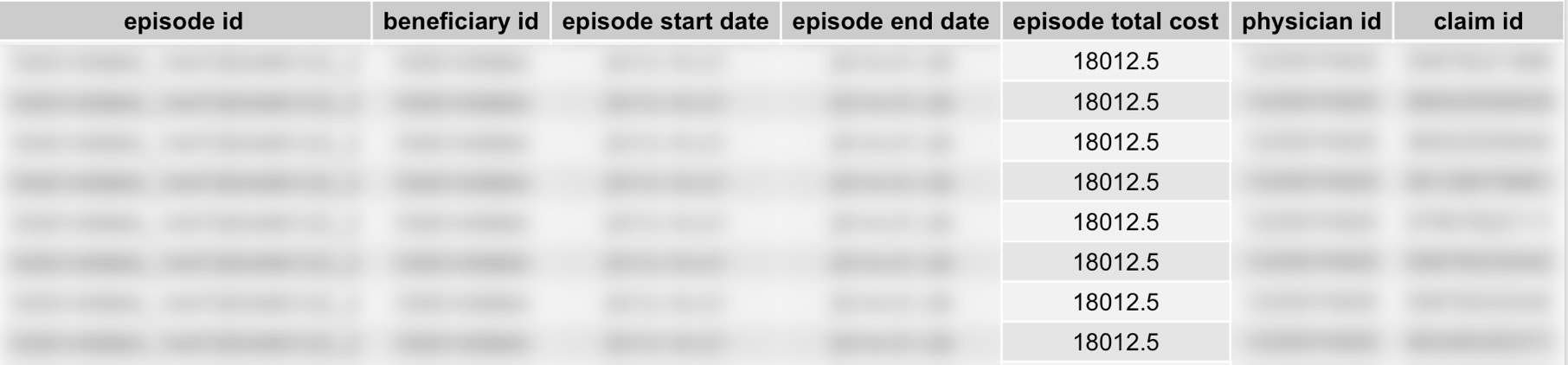
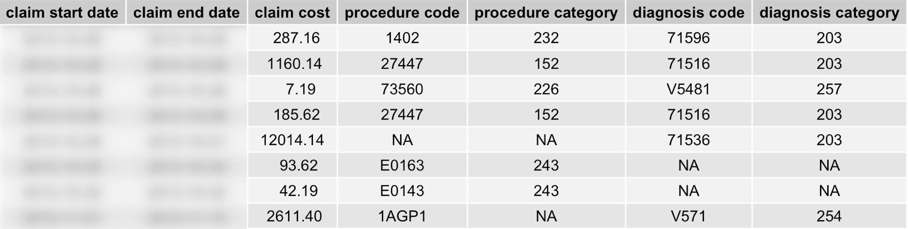
We use a data set of knee replacement claims provided by Cedar Gate Technologies. The data set contains claims records from 37 physicians and 205 unique beneficiaries (patients). There are 212 episodes, 5946 claims and 9254 entries. Each episode is a full claims record for a patient’s pathway from onset to rehabilitation and recovery. Each episode involves one physician, one beneficiary, a total cost, an episode start date, an episode end date, and a sequence of claims. Figure 2 gives a snapshot of several lines in the data set. Each entry contains the following attributes: episode id, beneficiary id, episode start date, episode end date, episode total cost, physician id, claim id, claim start date, claim end date, claim cost, procedure code, procedure category, diagnosis code, and diagnosis category. We have masked the sensitive information to protect the patient’s identity. In Appendix A we will discuss more details about the data set.
 |
 |
| (a) | (b) |

5.1 Projected Performances and Cross Validation
We aggregate the diagnosis categories into clusters by using the spectral state clustering method in Section 4, for . The partition map is further used to build a kernel function (3) for the state space . We view , the rank parameter used in state compression, as a measure of the model complexity. It is a tuning parameter that controls the tradeoff between model reduction error and overfitting error.
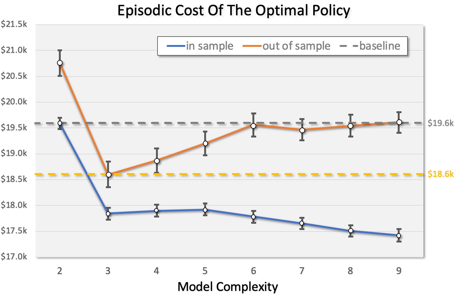
We conduct both in-sample and out-of-sample experiments. In in-sample experiments, we train the treatment policy to minimize cost over the entire data set, and test its performance on the same raw data. In out-of-sample experiments, we use 2-fold cross validation. We split the raw data set into two equal-size segments randomly, and compute the optimal policy using one segment and test its performance on the another segment. Each experiment is repeated randomly for 200,000 times and for all values of . The results are given in Figure 3. In particular, Figure 3 (a) shows the average cost per episode obtained from in-sample and out-of-sample experiments across values of , as well as their confidence intervels.
Note that according to (Japsen, 2016), hospitals have to keep their costs below $25,565 or they will face a financial charge. We define the episodic excessive cost premium as
In Figure 3 (b) we compare the episodic premium from the in-sample and out-of-sample experiments.
The results of Figure 3 are consistent with typical in-sample vs out-of-sample error curves for training machine learning models. It is expected that the in-sample error decreases monotonically as the model complexity increases, however, over-fitting would occur when is too large. The out-of-sample error curves show that over-fitting occurs when , therefore we pick to be the best model complexity for this data set. We take the out-of-sample performance at as the predicted performance of the optimized policy. In this case, the average cost per episode reduces by 7 percent and the excessive cost premium per episode reduces by 33 percent.
5.2 Cost Distribution and Tail Improvement
In Figure 4 we compare the histograms of episodic cost over the raw data and after optimization. The after-optimization cost distribution is obtained by simulation. The percentages of episodes costing over $30k are reduced significantly. Such a reduction mitigates the financial risk faced by healthcare providers, as they are penalized for costs over $25,565 according to CMS. The tail improvement is significant for reasons beyond financial risk. It is well known that excessive medical cost in medical treatment is highly correlated to unsuccessful cases, for example post-surgery complications often lead to extra surgeries, higher costs and traumatic discomforts. Therefore the tail cost reduction shown in Figure 4 suggests that the optimized clinical policy may reduce unnecessary medical complications and extra inpatient surgeries. The result implies that the proposed pipeline would not only reduce financial costs but also improve the quality of care.


5.3 Clinical Pathway Forecast Using The Optimal Policy
Now we have estimated the best clinical policy from data. Our model allows us to predict the entire clinical pathway of a typical knee replacement treatment. We simulate the knee replacement process under the optimized policy based on existing claim episodes. This generates 10,000 sample trajectories. Then based on the sample trajectories, we compute the empirical distribution of diagnosis categories per each day. Figure 5 (a) illustrates the distribution over states as time progresses, when the optimal policy is used.
Our model can also forecast the future clinical pathway of a patient from any given time and given state during the knee replacement episode. Figure 5 (b)(c)(d) illustrates the forecasted pathway from day 25, day 50, day 75, respectively, conditioned on the event that the current diagnosis belongs to the category of osteoarthritis. Figure 5 (e) illustrated the forecasted pathway from day 50, conditioned on the event that the current diagnosis belongs to the category of non-traumatic joint disorders. We see that the model is able to predict the conditional distributions of future diagnosis and treatments given any particular time and state of the treatment. The forecasts would be useful in terms of making physicians better informed before giving prescriptions.
6 Summary
This paper provides a reinforcement learning-based pipeline to optimize the knee replacement treatment from medical claims. It produces a clinical policy via intelligence crowdsourcing from experts and unsupervised state compression. Empirical validation suggests the optimized policy reduces the average cost per episode by $1,000, which implies a potential savings of millions each year in the US. We believe this result gives a proof-of-concept that reinforcement learning can significantly improve clinical decisions. For future work, we will focus on personalizing the knee replacement treatment by using data sets of large scales and higher-resolution models.
References
- Barnett et al., (2019) Barnett, M. L., Wilcock, A., McWilliams, J. M., Epstein, A. M., Joynt Maddox, K. E., Orav, E. J., Grabowski, D. C., and Mehrotra, A. (2019). Two-year evaluation of mandatory bundled payments for joint replacement. New England Journal of Medicine, 380(3):252–262.
- Barreto et al., (2016) Barreto, A., Precup, D., and Pineau, J. (2016). Practical kernel-based reinforcement learning. The Journal of Machine Learning Research, 17(1):2372–2441.
- Bertsekas et al., (1995) Bertsekas, D. P., Bertsekas, D. P., Bertsekas, D. P., and Bertsekas, D. P. (1995). Dynamic programming and optimal control, volume 1. Athena scientific Belmont, MA.
- Cabitza et al., (2018) Cabitza, F., Locoro, A., and Banfi, G. (2018). Machine learning in orthopedics: a literature review. Frontiers in bioengineering and biotechnology, 6.
- CMS, (2016) CMS (2016). Comprehensive care for joint replacement model. https://innovation.cms.gov/initiatives/CJR.
- Doorhof, (2018) Doorhof, D. (2018). Using reinforcement learning to improve clinical decision making in neonatal care. Master’s thesis.
- Duan et al., (2018) Duan, Y., Ke, Z. T., and Wang, M. (2018). State aggregation learning from markov transition data. arXiv preprint arXiv:1811.02619.
- Esteva et al., (2017) Esteva, A., Kuprel, B., Novoa, R. A., Ko, J., Swetter, S. M., Blau, H. M., and Thrun, S. (2017). Dermatologist-level classification of skin cancer with deep neural networks. Nature, 542(7639):115.
- Hinton et al., (2012) Hinton, G., Deng, L., Yu, D., Dahl, G., Mohamed, A.-r., Jaitly, N., Senior, A., Vanhoucke, V., Nguyen, P., Kingsbury, B., et al. (2012). Deep neural networks for acoustic modeling in speech recognition. IEEE Signal processing magazine, 29.
- Huber et al., (2019) Huber, M., Kurz, C., and Leidl, R. (2019). Predicting patient-reported outcomes following hip and knee replacement surgery using supervised machine learning. BMC medical informatics and decision making, 19(1):3.
- Japsen, (2016) Japsen, B. (2016). Medicare’s bundled fees hit knee, hip replacements.
- Jong and Stone, (2006) Jong, N. and Stone, P. (2006). Kernel-based models for reinforcement learning. In ICML Workshop on Kernel Machines and Reinforcement Learning. Citeseer.
- Kveton and Theocharous, (2013) Kveton, B. and Theocharous, G. (2013). Structured kernel-based reinforcement learning. In Twenty-Seventh AAAI Conference on Artificial Intelligence.
- Li et al., (2010) Li, L., Chu, W., Langford, J., and Schapire, R. E. (2010). A contextual-bandit approach to personalized news article recommendation. In Proceedings of the 19th international conference on World wide web, pages 661–670. ACM.
- Li, (2017) Li, Y. (2017). Deep reinforcement learning: An overview. arXiv preprint arXiv:1701.07274.
- Luo et al., (2016) Luo, J., Wu, M., Gopukumar, D., and Zhao, Y. (2016). Big data application in biomedical research and health care: a literature review. Biomedical informatics insights, 8:BII–S31559.
- Manning et al., (2014) Manning, C., Surdeanu, M., Bauer, J., Finkel, J., Bethard, S., and McClosky, D. (2014). The stanford corenlp natural language processing toolkit. In Proceedings of 52nd annual meeting of the association for computational linguistics: system demonstrations, pages 55–60.
- Martin, (2017) Martin, G. M. (2017). Patient education: Total knee replacement (arthroplasty)(beyond the basics). UpToDate. com.
- Miotto et al., (2017) Miotto, R., Wang, F., Wang, S., Jiang, X., and Dudley, J. T. (2017). Deep learning for healthcare: review, opportunities and challenges. Briefings in bioinformatics, 19(6):1236–1246.
- Mnih et al., (2015) Mnih, V., Kavukcuoglu, K., Silver, D., Rusu, A. A., Veness, J., Bellemare, M. G., Graves, A., Riedmiller, M., Fidjeland, A. K., Ostrovski, G., et al. (2015). Human-level control through deep reinforcement learning. Nature, 518(7540):529.
- Navarro et al., (2018) Navarro, S. M., Wang, E. Y., Haeberle, H. S., Mont, M. A., Krebs, V. E., Patterson, B. M., and Ramkumar, P. N. (2018). Machine learning and primary total knee arthroplasty: patient forecasting for a patient-specific payment model. The Journal of arthroplasty, 33(12):3617–3623.
- Nemati et al., (2016) Nemati, S., Ghassemi, M. M., and Clifford, G. D. (2016). Optimal medication dosing from suboptimal clinical examples: A deep reinforcement learning approach. In 2016 38th Annual International Conference of the IEEE Engineering in Medicine and Biology Society (EMBC), pages 2978–2981. IEEE.
- Olsen et al., (2010) Olsen, L., Saunders, R. S., Yong, P. L., et al. (2010). The healthcare imperative: Lowering costs and improving outcomes: Workshop series summary. National Academies Press.
- Ormoneit and Sen, (2002) Ormoneit, D. and Sen, Ś. (2002). Kernel-based reinforcement learning. Machine learning, 49(2-3):161–178.
- Parbhoo et al., (2017) Parbhoo, S., Bogojeska, J., Zazzi, M., Roth, V., and Doshi-Velez, F. (2017). Combining kernel and model based learning for hiv therapy selection. AMIA Summits on Translational Science Proceedings, 2017:239.
- Peng et al., (2018) Peng, X., Ding, Y., Wihl, D., Gottesman, O., Komorowski, M., Lehman, L.-w. H., Ross, A., Faisal, A., and Doshi-Velez, F. (2018). Improving sepsis treatment strategies by combining deep and kernel-based reinforcement learning. In AMIA Annual Symposium Proceedings, volume 2018, page 887. American Medical Informatics Association.
- Prasad et al., (2017) Prasad, N., Cheng, L.-F., Chivers, C., Draugelis, M., and Engelhardt, B. E. (2017). A reinforcement learning approach to weaning of mechanical ventilation in intensive care units. arXiv preprint arXiv:1704.06300.
- (28) Raghu, A., Komorowski, M., Ahmed, I., Celi, L., Szolovits, P., and Ghassemi, M. (2017a). Deep reinforcement learning for sepsis treatment. arXiv preprint arXiv:1711.09602.
- (29) Raghu, A., Komorowski, M., Celi, L. A., Szolovits, P., and Ghassemi, M. (2017b). Continuous state-space models for optimal sepsis treatment-a deep reinforcement learning approach. arXiv preprint arXiv:1705.08422.
- Russakovsky et al., (2015) Russakovsky, O., Deng, J., Su, H., Krause, J., Satheesh, S., Ma, S., Huang, Z., Karpathy, A., Khosla, A., Bernstein, M., et al. (2015). Imagenet large scale visual recognition challenge. International journal of computer vision, 115(3):211–252.
- Shickel et al., (2018) Shickel, B., Tighe, P. J., Bihorac, A., and Rashidi, P. (2018). Deep ehr: a survey of recent advances in deep learning techniques for electronic health record (ehr) analysis. IEEE journal of biomedical and health informatics, 22(5):1589–1604.
- Silver et al., (2017) Silver, D., Schrittwieser, J., Simonyan, K., Antonoglou, I., Huang, A., Guez, A., Hubert, T., Baker, L., Lai, M., Bolton, A., et al. (2017). Mastering the game of go without human knowledge. Nature, 550(7676):354.
- Sutton et al., (1998) Sutton, R. S., Barto, A. G., et al. (1998). Introduction to reinforcement learning, volume 135. MIT press Cambridge.
- Sutton et al., (2012) Sutton, R. S., Szepesvári, C., Geramifard, A., and Bowling, M. P. (2012). Dyna-style planning with linear function approximation and prioritized sweeping. arXiv preprint arXiv:1206.3285.
- Zhang and Wang, (2018) Zhang, A. and Wang, M. (2018). Spectral state compression of markov processes. arXiv preprint arXiv:1802.02920.
Appendix A Data
We use a data set of knee replacement claims from Cedar Gate Technologies. It is a healthcare analytics company that provides prescriptive tools to help healthcare organizations and insurance companies manage their costs and risks.
The data set contains claims records from 37 physicians and 205 unique beneficiaries (patients). It contains 212 episodes, 5946 claims and 9254 entries. Each episode is a full claims record for a patient’ pathway from onset to rehabilitation and recovery. Each episode involves one physician, one beneficiary, a total cost, an episode start date, an episode end date, and a sequence of claims.
Attributes: Each entry contains the following attributes: episode id, beneficiary id, episode start date, episode end date, episode total cost, physician id, claim id, claim start date, claim end date, claim cost, procedure code, procedure category, diagnosis code, diagnosis category.
Date: Each episode has one “episode start date" and one “episode end date", and each claim has one “claim start date" and one “claim end date". Most claims start and end on the same day. But still, there exists some claims whose “claim start date" and “claim end date" are different.
Claim: Each claims consists of diagnoses, procedures, a start date, an end date and a cost of the claim. There are 597 different procedures, 81 procedure categories, 542 different diagnoses, and 138 diagnosis categories in this data set. Almost all claims involves only one diagnosis and/or only one procedure. For example, see line 6 in Figure 2, where “NA" means the corresponding procedure or diagnosis does not exist. Some claims have more than one entries.
Beneficiaries and Physicians: There are 37 physicians and 205 beneficiaries in this data set. Each beneficiary is attributed to a unique physician.
Duration and Cost: The duration of episodes are all around 100 days, because knee replacement is a standardized and well-scheduled process. The number of claims per episode ranges from 8 to 56.
For confidentiality purposes, we are not allowed to disclose additional information about the data set.
Appendix B Training Details
In Section 4, we solve the problem (2) by applying the k-means method with 100 random initializations and choosing the one with the least sum of squares. In Section 5.1, we do in-sample experiments as following, Step 1: First get the optimal policy using the whole data, and then simulate it 400 times to calculate the average cost. Step 2: Repeat step 1 five hundreds times. The error bar is the 95% confidence interval of averages in Step 2. In out-of-sample experiments, Step 1: Split the whole data set into two equal-size segments randomly, and compute the optimal policy using one segments. Step 2: Use the optimal policy from step 1 to simulate episode cost on the remaining data 400 times, and get an average cost. Step 3: Repeat Step 1 and Step 2 five hundreds times. The error bar is the 95% confidence interval of averages in Step 3. In Section 5.2, we choose , and run the same experiments as in Section 5.1. In Section 5.3, we simulate 10,000 the knee replacement process under the optimized policy based on existing claim episodes from day 0, day 25, and day 75. Then based on the sample trajectories, we compute the empirical distribution of diagnosis categories per each day.