Forward scattering amplitudes of pp and pp̄ with crossing symmetry and scaling properties
Abstract
We analyse the pp and pp̄ elastic scattering amplitudes using the data of several CERN and FERMILAB experiments, revisiting ideas proposed by André Martin based on analytic continuation and crossing symmetry. Introducing a new form for the scaling function together with the analytical forms from COMPETE at we show that the data are consistent with the crossing symmetry of the scattering amplitudes from 23 GeV to 13 TeV for GeV2. Analiticity and crossing symmetry automatically satisfy the dispersion relations and their derivatives. The real part reproduces the zero predicted by Martin, which is crucial to describe with precision the differential cross section in the forward range at high energies. Since the free parameters of the model are energy independent, the analytical form of the amplitude allows predictions for intermediate and higher energies.
Keywords:
elastic scattering amplitudes, analyticity, crossing symmetry, dispersion relations, scaling, total cross sectionI Introduction of the model
Theoretical and phenomenological approaches for the description of pp and pp̄ elastic scattering aim to determine the dynamics and kinematical dependence of the amplitudes, described in terms of the two variables and . In Regge theory the rise of the hadronic total cross section can be described by the Pomeron trajectory linear in , with power dependence on in the case of a simple pole. However at high energies the growth of the total cross section guided by the Froissart bound Froissart and by the behaviour of the observed data can be parametrized as a quadratic form in such as , where we consider GeV, and we omit for simplicity. The form of the differential cross section depends on specific assumptions for the real and imaginary amplitudes, controled by dispersion relations (DR). In what follows we use the variable as a crossing symmetric variable, which coincides with the energy in the laboratory frame for .
In another treatment for very large energies in the forward region, if the real amplitude is neglected compared with the imaginary part, the scattering amplitude is suggested to follow a scaling dependence Deus, with where is a combination of and variables. Using the dependence combined with the scaling function the scattering amplitude is then written with the form,
| (1) |
The bounds and constraints of were formally studied long ago Deus in the context of axiomatic field theory, giving , where is constant and the scaling variable is . The cross section corresponding to Eq.(1) is not invariant under the transformation, (crossing symmetry). Following A. Martin Martin_Real, in order to define a complex crossing symmetric function, Eq.(1) can be modified to
| (2) |
The extension of in the complex plane changes the scaling variable to a complex variable which transforms the scaling function in a complex quantity.
However, it is not obvious that at large energies these amplitudes, with both crossing and scaling, are well satisfied. Attempts have been made in this direction to analyse ISR energies with where and are free parameters to be fitted at each energy MenonFagundes. To test the ideas of crossing and scaling we propose in the current work a modified model for the forward scattering at high energies using the analytical crossing symmetric forms explored by Block and Cahn Block:1985 and used in the COMPETE parametrization COMPETE
| (3) |
It is easy to check that the LHS of Eqs.(3) are analytical by the interchange of keeping the forms crossing symmetric. Since we are interested in a high energy region (starting from ISR energies) the mass term on the LHS of Eqs.(3) can be safely neglected and the RHS approximation is justified. Crossing symmetry imposes , but here we let free for a test against the data. The subscripts (+) and (-) refer to even and odd terms under crossing symmetry. We generalize Eq.(2) writing
| (4) |
where are refereed to pp/pp̄ respectively. The parameters , , , , , and are fixed numbers for all energies.
The dependence is embedded in the complex scaling variable defined as
| (5) |
with , , , as fixed quantities, while is allowed to have energy dependence. We assume a complex scaling function
| (6) |
We can also approximate and we re-write the above amplitudes using the variable keeping the same analytical dependence
| (7) |
Separating the real and imaginary parts we have
| (8) |
| (9) |
and
| (10) |
| (11) |
We adopt the suggestion from COMPETE parametrization COMPETE for the amplitudes at with the same given parameters , , , , , and , while is left as a free parameter to test the crossing symmetry. The parameters that dictate the forward dependence of the differential cross section are , , , (energy independent) while the energy dependence of is obtained from differential cross section data.
The separation of the real and imaginary gives
| (12) |
and
| (13) |
The complex amplitude can be written in the compact form
| (14) |
where is the forward mixing angle between and the unity. The total cross sections for pp/pp̄ are given by the optical theorem
| (15) |
and the the ratios of the amplitudes at are
| (16) |
Note that Eq.(14) has trigonometric functions which make the sum of the absolute square of the real and imaginary nuclear parts as a simple exponential function
| (17) |
which does not describe well the forward scattering data. To improve we add to the real part a shape function
| (18) |
which is zero for and does not affect crossing symmetry. The amplitude is then written as
| (19) |
The sum of the squared amplitudes is
| (20) |
A more complete dependence of may also contain terms with negative parity, for example, the Odderon (for a review see Carlo) which may be important for larger values, specially at the dip region.
The real part is approximatly linear in for small and accounts for a zero with an energy dependence, which corresponds to Martin’s zero Martin, while in the imaginary amplitude there is no zero, since this model does not intend to describe the dip region. This can be seen due to the lack of the minus sign in the rotation matrix Eq.(14).
The derivatives of the logarithm of the real and imaginary amplitudes at are respectively,
| (21) |
and
| (22) |
where and are refereed to as the effective slopes of the real and imaginary amplitudes. These derivatives determine the average slope of the differential cross section at , which in terms of Eqs. (16), (21) and (22) is given by
| (23) |
The high energy behaviour () of pp and pp̄ total cross section implies for high energies Kinoshita, which compared with Eq.(16) automatically imposes . The exact forms of dispersion relations can be computed for the amplitudes and their derivatives according to our recent mathematical results DDR_EXACT. However, the energy dependence of the parameter needs to be studied in detail.
We fix the parameters mb, mb, mb, mb, and , according to PDG parametrization (with some flexibility in the numerical values), living as a free parameter. The parameters GeV-2, GeV-2, GeV-2 and GeV-2 are fixed according to the global fit of all data analysed. The parameter responsible for the crossing symmetry is stable in most of the studied energies and is compatible with . We leave as a free parameter. We fit the experimental data from FNAL Kuz, ISR Amaldi; Amos, Spp̄SAugier, E710E710 and LHC A7; A8; T7; T8; T13, covering a range of from 23 GeV to 13 TeV, using
| (24) |
where the amplitude is
| (25) |
The Coulomb interaction together with the proton form factor is written for pp and pp̄ respectively
| (26) |
with (the fine structure constant) and GeV2 is the electromagnetic form factor scale.
In spite of many attempts to calculate the relative Coulomb phase , it is still a open problem. The most used approaches such as West-Yennie, Slov’ev, Cahn and Kundrat phases, were derived based on strong assumptions. First the WY approach was based in the Feynman diagrams considering the strong interactions as an effective vertex (similarly with Slov’ev). The electromagnetic Feynman diagrams were expanded assuming the proton as a point like-particle. On the other hand Cahn’s approach which was based on the additivity of the eikonal functions for the Coulomb and strong interactions is not more than a guess. The two interactions have no reason the be additive in terms of eikonals. Besides the electromagnetic form factor is imposed by hand. In this sense, as explained in our previous work the relative Coulomb phase could be tested as zero without problems us.
II COMPARISON WITH DATA
The datasets have been analysed in limited -range () GeV2 chosen appropriately in order to account for the stability of , which in our analysis is manifestly positive. The positiveness of the real amplitude for near zero was recently proved by A. Martin and T. T. Wu Martin_2017 and this supports our results for .
We obtain that all datasets analysed are well represented by our model with reasonable small . The fits show that is compatible with for all datasets. This parameter is related with the phase of the complex nuclear amplitude. Thus, if we consider as an input in Eq.(4) the scattering amplitude becomes crossing symmetric under for fixed .
The energy dependence of , shown in the LHS of Fig.1, can be parametrized with a power of as
| (27) |
with the parameters , and . These parameters seem to be constant with energy, supporting the idea of the existence of a complex scaling function . The regular dependence of is remarkable, and for very large energies this quantity tends to stay constant around . The RHS of Fig.1 shows the values of H obtained for the analysed energies. We see that the numerical values fluctuates according to different normalizations of the experiments, but on average it stays constant. In this sense in order to make some predictions we fix the average value of mb.
In Table 1 we show the obtained parameters , for all analysed energies and the extracted forward quantities , , , . We also show predictions for the energies 0.2, 0.9, 2.76, 14 and 57 TeV.
An important feature of the model is Martin’s zero in the real part of pp and pp̄ Martin. Setting Eq.(12) equals zero we obtain the solution for Martin’s zero. However, since we are working in very small the trigonometric and the shape functions can be expanded in powers of . We take the leading terms in the real amplitude and we write the position of the zero
| (28) |
Fig.2 shows the zeros of Martin for pp and pp̄. For ISR energies the position of the zero moves to higher , but at TeV energies it starts to decrease as predicted by the theorem of MartinMartin.
Fig.3 shows the amplitudes for pp and pp̄ at similar energies about (52 GeV). The real parts are positive at and have zeros near the origin. The magnitude of the imaginary part is much larger than the real part for low values.
Fig.4 shows the ratio for 23, 44, 52, 62, 540, 1800 GeV for both pp and pp̄. This ratio removes from the differential cross section the simple exponential behaviour, which is essentially dictated by the imaginary part, allowing to investigate with detail the structure of the real amplitude. We observe that the curvature at all energies is created by the zero of the real part together with and the magnitude of the real slope.
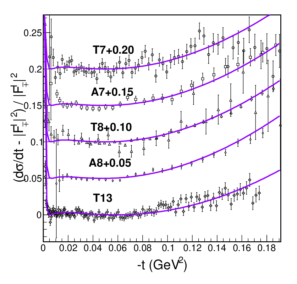
The LHS of Fig. 5 shows the ratio for LHC energies 7, 8 and 13 TeV. As in the previous figures involving the data we add factors multiples of 0.05 to separate the data. For these LHC energies we note that a ’soft peak’ structure is presented in the very forward region. In the RHS figure we show the real and imaginary amplitudes at 13 TeV, but this time we include the Coulomb amplitude. For pp scattering the Coulomb amplitude is negative while the real nuclear part is positive. The interplay between them produces a zero in the very forward range which can be seen in the figure.
| parameters | derived quantities | |||||||
| Refs | ||||||||
| (GeV) | (mb) | (mb) | (GeV | (mb) | ||||
| pp | ||||||||
| 23.882 | 0.3110.002 | 0.16 (fix) | 39.57 | 0.034 | 11.77 | 7.27 | 90.7/62 | Kuz |
| 30.6 | 0.2920.001 | 0.15220.001 | 39.79 | 0.049 | 12.23 | 7.03 | 94.1/68 | Amaldi |
| 44.7 | 0.2910.0004 | 0.144 (fix) | 41.51 | 0.077 | 13.12 | 7.08 | 87.3/67 | Amaldi |
| 52.8 | 0.28940.0003 | 0.13830.0003 | 42.41 | 0.088 | 13.26 | 7.30 | 245/88 | Amaldi |
| 62.5 | 0.28120.0005 | 0.13040.0004 | 42.76 | 0.092 | 13.15 | 7.49 | 111.1/62 | Amaldi |
| 200* | 0.2887 (fix) | 0.106 (fix) | 52.05 | 0.133 | 14.61 | 9.94 | - | |
| 900* | 0.2887 (fix) | 0.085 (fix) | 68.38 | 0.145 | 16.43 | 15.15 | - | |
| 2760* | 0.2887 (fix) | 0.076 (fix) | 84.04 | 0.143 | 18.23 | 20.51 | - | |
| 7000 | 0.28950.0003 | 0.07350.0002 | 99.51 | 0.138 | 20.39 | 25.57 | 74.4/59 | T7 |
| 7000 | 0.27640.0002 | 0.07070.0001 | 95.43 | 0.136 | 19.90 | 24.11 | 42.9/33 | A7 |
| 8000 | 0.29030.0001 | 0.06940.0001 | 102.12 | 0.137 | 19.65 | 27.99 | 72.5/58 | T8 |
| 8000 | 0.27350.0001 | 0.06980.0001 | 96.74 | 0.135 | 20.11 | 24.51 | 28.8/25 | A8 |
| 13000 | 0.29130.0001 | 0.06730.0001 | 111.43 | 0.134 | 20.99 | 31.11 | 149.4/126 | T13 |
| 14000* | 0.2887 (fix) | 0.067 (fix) | 112.65 | 0.132 | 21.13 | 31.15 | - | |
| 57000* | 0.2887 (fix) | 0.063 (fix) | 141.59 | 0.123 | 24.19 | 42.93 | - | |
| pp̄ | ||||||||
| 30.4 | 0.29940.003 | 0.15 (fix) | 41.32 | 0.076 | 12.05 | 7.73 | 22.4/25 | Amos |
| 52.6 | 0.29710.001 | 0.138 (fix) | 43.44 | 0.102 | 13.24 | 7.69 | 29.9/27 | Amos |
| 62.3 | 0.29380.003 | 0.132 0.004 | 44.13 | 0.107 | 13.32 | 7.89 | 19.9/15 | Amos |
| 540 | 0.29300.0004 | 0.09010.0003 | 62.95 | 0.145 | 15.65 | 13.52 | 164.9/97 | Augier |
| 1800 | 0.27060.001 | 0.07710.0004 | 73.71 | 0.141 | 17.19 | 16.78 | 43.8/53 | E710 |



The difficulties in the determination of the parameter from the data are well known for various phenomenological models. A proper determination depends on the analytical form used to parametrize the nuclear interaction and on the interference with the Coulomb interaction which is still an open problem. The quality of the experimental data in the interference region is crucial for this purpose. In the present model the analytical connection between the real and imaginary parts controls the fit instabilities, constraining from dispersion relations. In this sense we understand that the Odderon term is not necessary to explain the LHC forward data. Other analysis also consider only the even (Pomeron) term to explain the forward data Donachie.
III Conclusion
In recent studies of the LHC data on pp elastic scattering with independent real and imaginary amplitudes us, specific features of the real part, such as the position of the zero and the magnitude and sign of the amplitudes were investigated, and the parameters were determined with high precision. In the present work we discuss properties of analyticity and crossing symmetry of the amplitudes in the forward regime. It is important to remark that the real and imaginary amplitudes Eq.(14), when expanded to small values have similar forms on compared with the amplitudes in previous work us. The main difference is in the imaginary part of us which contains an additional linear factor on that accounts for the existence of the dip in the differential cross section for larger values. This difference influences the parameters of the real part giving small modifications in the quantities such as and the effective slope .
Advocated in Deus, the geometric scaling in hadronic collisions is achieved when the and dependence can be written in terms of a single variable . Until the LHC energies the experimental data on elastic pp and pp̄ does not follow the geometric scaling. One way to observe this mismatch is through the ratio between elastic and total cross section deDeus:2013 that should be constant with the energy and clearly this is not the case with the existing collider data. Since in our model we can extrapolate our results to higher energies we can calculate the asymptotic ratio . However we are aware of the limitations of the model at very high energies and we do not claim that this is the final answer. Usually the scaling variable is defined to be a real function , but this is an arbitrary choice. We define a complex variable such that the scaling behaviour is obeyed for all analysed energies, i.e., the ratio is function of a single variable starting already from ISR energies. Attempts have been made to extract universal properties of the position of the dip in the elastic differential cross section by the re-definition of the scaling variable Fagundes:2014 achieving relative success. In the microscopic level the geometric scaling was observed in Deep Inelastic Scattering for cross section Stasto. In this process the scaling variable is given as , which is a combination of the virtuality of the photon and the saturation scale for gluons . In principle there should exist a connection between the gluon saturation and the Froissart bound of the total hadronic cross sections. Works in this direction Froissart_Saturation have been developed but so far, no conclusive answer was given for pp or pp̄ processes.
The impact parameter space is interesting to investigate the geometrical features of the hadronic interactions and the matter distribution within the proton. However the impact parameter is not directly observed from the data and in order to obtain a complete profile function starting from the momentum space, one should be able to provide the complete dependence of the elastic amplitudes. Recently there have been some interest in the properties of the geometric space and some authors b-space claim the existence of a peripheral behaviour in the proton structure in the LHC energies called hollowness. In this description the inelastic profile functions at is reduced as the energy increases meaning that the periphery of the proton is more active. It is important however to stress that the profile functions are not necessarily genuine differential cross sections in b-space, but, since they behave monotonically and continuously in b, it is natural to relate these profile functions with the geometric dependence of the interaction. In the present work since we are interested in the very forward region the corresponding b-space amplitudes are not completely developed. Once we incorporate the larger dependence in our model we will be able to discuss the physical properties of the b-space.
To summarize, in the present work we propose a phenomenological tool to interpolate and extrapolate the experimental data, obeying crossing symmetry, dispersion relations and allowing the existence of a geometric scaling at asymptotic energies. This is a very useful information since historically some experiments give different results at the same energy (see Totem and Atlas for pp at 8 GeV and Fermilab for pp̄ at 1.8 GeV). In addition we present precise predictions for the energies 200 and GeV which were recently released in the EDS Blois conference blois giving the results mb, mb and GeV-2 and we see that those results are predicted in the present work.
Acknowledgments
The author thanks Erasmo Ferreira, Takeshi Kodama and Tri Nang Pham for useful discussions and reading of the manuscript. The author also thanks the Brazilian agency CAPES for financial support.
References
References
- (1) M Froissart, Phys. Rev. 123 (1961) 1053.
- (2) G. Auberson, T. Kinoshita and A. Martin, Phys. Rev. D 3 (1971) 12; J. Dias De Deus, Nuc. Phys. B 59 (1973) 231; I. Bautista and J. Dias De Deus, Phys. Lett. B 718 (2013) 1571.
- (3) A. Martin, Lett. Nuovo Cim. 7 (1973) 811.
- (4) D. Fagundes and M. Menon, Int. J. Mod. Phys. A 26 (2011) 3219.
- (5) M. M. Block and R. N. Cahn, Rev. Mod. Phys 57 (1985) 563.
- (6) COMPETE Collaboration, Phys. Rev. Lett. 89 (2002) 201801 .
- (7) C. Ewerz, hep-ph/0306137 (2003).
- (8) A. Martin, Phys. Lett. B 404 (1997) 137.
- (9) N. N. Khuri and T. Kinoshita, Phys. Rev. B 137 (1965) 720.
- (10) E. Ferreira and J. Sesma, J. Math. Phys. 49 (2008) 033504; E. Ferreira and J. Sesma, J. Math. Phys. 54 (2013) 033507; E. Ferreira, A. K. Kohara and J. Sesma, Phys. Rev. D 98 (2018) 094029;
- (11) A. A. Kuznetsov et al. , Sov. J. Nucl. Phys. 33, (1981) 74, and Yad. Fiz. 33, (1981) 142.
- (12) U. Amaldi and K.R. Schubert, Nucl. Phys. B 166, (1980) 301.
- (13) N. Amos, et al., Nuc. Phys. B 262 (1985) 689.
- (14) C. Augier et al. , [UA4/2 Coll.] , Phys. Lett. B 316 (1993) 448.
- (15) N. A. Amos et al. [E-710 Coll.], Phys. Lett. B 247 (1990) 127.
- (16) G. Aad et al. [ATLAS Coll.], Nucl. Phys. B 889 (2014) 486.
- (17) G. Aad et al. [ATLAS Coll.], Phys. Lett. B 761 (2016) 158.
- (18) G. Antchev et al. [TOTEM Coll.], Eurphys. Lett. 101 (2013) 21002.
- (19) G. Antchev et al. [TOTEM Coll.], Eur. Phys. J. C. 16 (2016) 661; Nucl. Phys. B 899 (2015) 527.
- (20) G. Antchev et al, Eur. Phys. J. C 79 (2019) 785.
- (21) L. D. Solov’ev, Zh. Eksperim. i Teor. Fiz. 49, 292 (1965); Soviet Phys. JETP 22, 205 (1966); G. B. West and D. R. Yennie, Phys. Rev. 172, 1413 (1968); R. Cahn, Zeit. Phys. C 15, 253 (1982); V. Kundrát and M. Lokajic̃ek, Zeit. Phys. C 63, 619 (1994).
- (22) A. K. Kohara, E. Ferreira, T. Kodama and M. Rangel, Eur. Phys. J. C 77 (2017) 877; A. K. Kohara, E. Ferreira, and M. Rangel, Phys. Lett. B 789 (2019) 1.
- (23) A. Martin and T. T. Wu, Phys. Rev. D 97 (2018) 014011.
- (24) A. Donnachie and P. V. Landshoff, arXiv:1904.11218 (2019).
- (25) I. Bautista and J. D. de Deus, Phys. Lett. B 718 (2013) 1571.
- (26) G. Pancheri et al, Nuovo Cim. C 037 (2014) 2, 179.
- (27) A. M. Stasto, K. J. Golec-Biernat and J. Kwiecinski, Phys. Rev. Lett. 86 (2001) 596.
- (28) E. Ferreiro, E. Iancu, K. Itakura, L. McLerran, Nucl.Phys. A 710 (2002) 373; F. Carvalho, F.O. Duraes, V.P. Goncalves andF.S. Navarra, Mod. Phys. Lett. A 23 (2008) 2847.
- (29) W. Broniowski, L. Jenkovszky, E. R. Arriola and I. Szanyi, Phys. Rev. D98 (2018) 074012; J. L. Albacete and A. Soto, Phys. Lett. B 770 (2017) 149.
- (30) W. Guryn, B. Pawlik, Work presented at EDS Blois 2019, June 23-29, 2019, Quy Nhon, Vietnam; ”https://indico.cern.ch/event/783891/contributions/3384036/attachments/1868096/3072691/EDS-Blois-2019-final.pdf”