Convergence of Learning Dynamics in Stackelberg Games

\nameTanner Fiez \emailfiezt@uw.edu Affiliation: \addrDepartment of Electrical and Computer Engineering Affiliation: University of Washington \nameBenjamin Chasnov \emailbchasnov@uw.edu Affiliation: \addrDepartment of Electrical and Computer Engineering Affiliation: University of Washington \nameLillian J. Ratliff \emailratliffl@uw.edu Affiliation: \addrDepartment of Electrical and Computer Engineering Affiliation: University of Washington

Abstract

This paper investigates the convergence of learning dynamics in Stackelberg games. In the class of games we consider, there is a hierarchical game being played between a leader and a follower with continuous action spaces. We establish a number of connections between the Nash and Stackelberg equilibrium concepts and characterize conditions under which attracting critical points of simultaneous gradient descent are Stackelberg equilibria in zero-sum games. Moreover, we show that the only stable critical points of the Stackelberg gradient dynamics are Stackelberg equilibria in zero-sum games. Using this insight, we develop a gradient-based update for the leader while the follower employs a best response strategy for which each stable critical point is guaranteed to be a Stackelberg equilibrium in zero-sum games. As a result, the learning rule provably converges to a Stackelberg equilibria given an initialization in the region of attraction of a stable critical point. We then consider a follower employing a gradient-play update rule instead of a best response strategy and propose a two-timescale algorithm with similar asymptotic convergence guarantees. For this algorithm, we also provide finite-time high probability bounds for local convergence to a neighborhood of a stable Stackelberg equilibrium in general-sum games. Finally, we present extensive numerical results that validate our theory, provide insights into the optimization landscape of generative adversarial networks, and demonstrate that the learning dynamics we propose can effectively train generative adversarial networks.

1 Introduction

Tools from game theory now play a prominent role in machine learning. The emerging coupling between the fields can be credited to the formulation of learning problems as interactions between competing algorithms and the desire to characterize the limiting behaviors of such strategic interactions. Indeed, game theory provides a systematic framework to model the strategic interactions found in modern machine learning problems.

A significant portion of the game theory literature concerns games of simultaneous play and equilibrium analysis. In simultaneous play games, each player reveals the strategy they have selected concurrently. The solution concept often adopted in non-cooperative simultaneous play games is the Nash equilibrium. In a Nash equilibrium, the strategy of each player is a best response to the joint strategy of the competitors so that no player can benefit from unilaterally deviating from this strategy.

The study of equilibrium gives rise to the question of when and why the observed play in a game can be expected to correspond to an equilibrium. A common explanation is that an equilibrium emerges as the long run outcome of a process in which players repeatedly play a game and compete for optimality over time [22]. Consequently, an important topic in the study of learning in games is the convergence behavior of learning algorithms reflecting the underlying game dynamics. Adopting this viewpoint and analyzing so-called ‘natural’ dynamics [7] often provides deep insights into the structure of a game. Moreover, a firm understanding of the structure of a game can inform how to design learning algorithms strictly for computing equilibria. Seeking equilibria via computationally efficient learning algorithms is an equally important perspective on equilibrium analysis [22].

The classic objectives of learning in games are now being widely embraced in the machine learning community. While not encompassing, the prevailing research areas epitomizing this phenomenon are adversarial training and multi-agent learning. A considerable amount of this work has focused on generative adversarial networks (GANs) [23]. Finding Nash equilibria in GANs is challenging owing to the complex optimization landscape that arises when each player in the game is parameterized by a neural network. Consequently, significant effort has been spent lately on developing principled learning dynamics for this application [42, 40, 25, 39, 3, 37]. In general, this line of work has analyzed learning dynamics designed to mitigate rotational dynamics and converge faster to stable fixed points or to avoid spurious stable points of the dynamics and reach equilibria almost surely. In our work, we draw connections to this literature and believe that the problem we study gives an under-explored perspective that may provide valuable insights moving forward.

Characterizing the outcomes of competitive interactions and seeking equilibria in multi-agent learning gained prominence much earlier than adversarial training. However, following initial works on this topic [35, 24, 27], scrutiny was given to the solution concepts being considered and the field cooled [56]. Owing to the arising applications with interacting agents, problems of this form are being studied extensively again. There has been a shift toward analyzing gradient-based learning rules, in part due to their scalability and success in single-agent reinforcement learning, and rigorous convergence analysis [60, 3, 33, 21, 38].

The progress analyzing learning dynamics and seeking equilibria in games is promising, but the work has been narrowly focused on simultaneous play games and the Nash equilibrium solution concept. There are many problems exhibiting a hierarchical order of play between agents in a diverse set of fields such as human-robot collaboration and interacting autonomous systems in artificial intelligence [45, 36, 20, 54], mechanism design and control [19, 51, 52], and organizational structures in economics [13, 2]. In game theory, this type of game is known as a Stackelberg game and the solution concept studied is called a Stackelberg equilibrium.

In the simplest formulation of a Stackelberg game, there is a leader and a follower that interact in a hierarchical structure. The sequential order of play is such that the leader is endowed with the power to select an action with the knowledge that the follower will then play a best-response. Specifically, the leader uses this knowledge to its advantage when selecting a strategy.

In this paper, we study the convergence of learning dynamics in Stackelberg games. Our motivation stems from the emergence of problems in which there is a distinct order of play between interacting learning agents and the lack of existing theoretical convergence guarantees in this domain. The dynamics analyzed in this work reflect the underlying game structure and characterize the expected outcomes of hierarchical game play. The rigorous study of the learning dynamics in Stackelberg games we provide also has implications for simultaneous play games relevant to adversarial training.

Contributions.

We formulate and study a novel set of gradient-based learning rules in continuous, general-sum games that emulate the natural structure of a Stackelberg game. Building on work characterizing a local Nash equilibrium in continuous games [50], we define the differential Stackelberg equilibrium solution concept (Definition 4), which is a local notion of a Stackelberg equilibrium amenable to computation. An analogous local minimax equilibrium concept was developed concurrently with this work, but strictly for zero-sum games [28]. Importantly, the equilibrium notion we present generalizes the local minimax equilibrium concept to general-sum games. In our work, we draw several connections between Nash and Stackelberg equilibria for the class of zero-sum games, which can be summarized as follows:

•

We show in Proposition 2 that stable Nash equilibria are differential Stackelberg equilibria in zero-sum games. Concurrent with our work, Jin et al. 2019 equivalently show that local Nash equilibria are local minimax equilibria. This result indicates learning dynamics seeking Nash equilibria are simultaneously seeking Stackelberg equilibria.
•

We reveal that there exist stable attractors of simultaneous gradient play that are Stackelberg equilibria and not Nash equilibria. Moreover, in Propositions 3 and 4 we give necessary and sufficient conditions under which the simultaneous gradient play dynamics can avoid Nash equilibria and converge to Stackelberg equilibria. To demonstrate the relevancy to deep learning applications, Propositions 5 and 6 specialize the general necessary and sufficient conditions from Propositions 3 and 4 to GANs satisfying the realizable assumption [43], which presumes the generator is able to create the underlying data distribution. This set of results has implications for the optimization landscape in GANs as we explore in our numerical experiments.

Our primary contributions concern the convergence behavior of the gradient-based learning rules we formulate that mirror the Stackelberg game structure. These contributions can be summarized as follows:

•

We demonstrate in Proposition 1 that the only stable critical points of the Stackelberg gradient dynamics are Stackelberg equilibria in zero-sum games. This is in contrast to the simultaneous gradient play dynamics, which can be attracted to non-Nash critical points in zero-sum games. This insight allows us to define a gradient-based learning rule for the leader while the follower plays a best response for which each attracting critical point is a Stackelberg equilibria in zero-sum games. As a result, the learning rule provably converges to an equilibria given an initialization in the region of attraction of a stable critical point. A formal exposition of this set of dynamics and results is provided in Section 3.1.
•

Leveraging the Stackelberg game structure, for general-sum games, we formulate a gradient-based learning rule in which the leader and follower have an unbiased estimator of their gradient so that updates are stochastic.
•

In Section 3.2, we consider a formulation in which the follower uses a gradient-play update rule instead of an exact best response strategy and propose a two-timescale algorithm to learn Stackelberg equilibria. We show almost sure asymptotic convergence to Stackelberg equilibria in zero-sum games and to stable attractors in general-sum games; a finite-time high probability bound for local convergence to a neighborhood of a stable Stackelberg equilibrium in general-sum games is also given.
•

We present this paper with a single leader and a single follower, but this is only for ease of presentation. The extension to $N$ followers that play in a staggered hierarchical structure or simultaneously is in Appendix F; equivalent results hold with some additional assumptions.

Finally, we present several numerical experiments in Section 4, which we now detail:

•

We present a location game on a torus and a Stackelberg duopoly game. The examples are general-sum games with equilibrium that can be solved for directly, allowing us to numerically validate our theory. The games demonstrate the advantage the leader gains from the hierarchical order of play compared to the simultaneous play versions of the games.
•

We evaluate the Stackelberg learning dynamics as a GAN training algorithm. In doing so, we find that the leader update removes rotational dynamics and prevents the type of cycling behavior that plagues simultaneous gradient play. Moreover, we discover that the simultaneous gradient dynamics can empirically converge to non-Nash attractors that are Stackelberg equilibria in GANs. The generator and the discriminator exhibit desirable performance at such points, indicating that Stackelberg equilibria can be as desirable as Nash equilibria. Lastly, the Stackelberg learning dynamics often converge to non-Nash attractors and reach a satisfying solution quickly using learning rates that can cause the simultaneous gradient descent dynamics to cycle.

Related Work.

The perspective we explore on analyzing games in which there is an order of play or hierarchical decision making structure has been generally ignored in the modern learning literature. However, this viewpoint has long been researched in the control literature on games [5, 47, 48, 29, 4]. Similarly, work on bilevel optimization [17, 16, 59] adopts this perspective.

The select few recent works in the machine learning literature on learning in games considering a hierarchical decision-making structure exclusively focus on zero-sum games [42, 28, 34, 46, 18], unlike our work, which extends to general-sum games. A noteworthy paper in the line of work in the zero-sum setting adopting a min-max perspective was the introduction of unrolled GANs [42]. The authors consider a timescale separation between the generator and discriminator, giving the generator the advantage as the slower player. This work used the Schur complement structure presented in Danskin 1967, Danskin 1966 to define a minimax solution of a zero-sum game abstraction of an adversarial training objective. Essentially the discriminator is allowed to perform a finite roll-out in an inner loop of the algorithm with multiple updates; this process is referred to as ‘unrolling’. It is (informally) suggested that, using the results of Danskin 1967, Danskin 1966, as the roll-out horizon approaches infinity, the discriminator approaches a critical point of the cost function along the discriminators axis given a fixed generator parameter configuration.

The unrolling procedure has the same effect as a deterministic timescale separation between players. Formal convergence guarantees to minimax equilibria in zero-sum games characterizing the limiting behavior of simultaneous individual gradient descent with timescale separation were recently obtained [28, 34]. While related, simultaneous individual gradient play with time-scale separation is a distinct set of dynamics that departs from the dynamics we propose that reflect the Stackelberg game structure.

It is also worth pointing out that the multi-agent learning papers of Foerster et al. 2018 and Letcher et al. 2019 do in some sense seek to give a player an advantage, but nevertheless focus on the Nash equilibrium concept in any analysis that is provided.

Organization.

In Section 2, we formalize the problem we study and provide background material on Stackelberg games. We then draw connections between learning in Stackelberg games and existing work in zero-sum and general sum-games relevant to GANs and multi-agent learning, respectively. In Section 3, we give a rigorous convergence analysis of learning in Stackelberg games. Numerical examples are provided in Section 4 and we conclude in Section 5.

2 Preliminaries

We leverage the rich theory of continuous games and dynamical systems in order to analyze algorithms implemented by agents interacting in a hierarchical game. In particular, each agent has an objective they want to selfishly optimize that depends on not only their own actions but also on the actions of their competitor. However, there is an order of play in the sense that one player is the leader and the other player is the follower¹¹ 1 While we present the work for a single leader and a single follower, the theory extends to the multi-follower case (we discuss this in Appendix F) and to the case where the single leader abstracts multiple cooperating agents.. The leader optimizes its objective with the knowledge that the follower will respond by selecting a best response. We refer to algorithms for learning in this setting as hierarchical learning algorithms. We specifically consider a class of learning algorithms in which the agents act myopically with respect to their given objective and role in the underlying hierarchical game by following the gradient of their objective with respect to their choice variable.

To substantiate this abstraction, consider a game between two agents where one agent is deemed the leader and the other the follower. The leader has cost $f_{1}:X\rightarrow\mathbb{R}$ and the follower has cost $f_{2}:X\rightarrow\mathbb{R}$ , where $X=X_{1}\times X_{2}$ with the action space of the leader being $X_{1}$ and the action space of the follower being $X_{2}$ . The designation of ‘leader’ and ‘follower’ indicates the order of play between the two agents, meaning the leader plays first and the follower second. The leader and the follower need not be cooperative. Such a game is known as a Stackelberg game.

2.1 Stackelberg Games

Let us adopt the typical game theoretic notation in which the player index set is $\mathcal{I}$ and $x_{-i}=(x_{j})_{j\in\mathcal{I}/\{i\}}$ denotes the joint action profile of all agents excluding agent $i$ . In the Stackelberg case, $\mathcal{I}=\{1,2\}$ where player $i=1$ is the leader and player $i=2$ is the follower. We assume throughout that each $f_{i}$ is sufficiently smooth, meaning $f_{i}\in C^{q}(X,\mathbb{R})$ for some $q\geq 2$ and for each $i\in\mathcal{I}$ .

The leader aims to solve the optimization problem given by

\min_{x_{1}\in X_{1}}\Big\{f_{1}(x_{1},x_{2})\big|\ x_{2}\in\arg\min_{y\in X_{2}}f_{2}(x_{1},y)\Big\}

and the follower aims to solve the optimization problem $\min_{x_{2}\in X_{2}}f_{2}(x_{1},x_{2})$ . As noted above, the learning algorithms we study are such that the agents follow myopic update rules which take steps in the direction of steepest descent with respect to the above two optimizations problems, the former for the leader and the latter for the follower.

Before formalizing these updates, let us first discuss the equilibrium concept studied for simultaneous play games and contrast it with that which is studied in the hierarchical play counterpart. The typical equilibrium notion in continuous games is the pure strategy Nash equilibrium in simultaneous play games and the Stackelberg equilibrium in hierarchical play games. Each notion of equilibria can be characterized as the intersection points of the reaction curves of the players [4].

Definition 1 (Nash Equilibrium).

The joint strategy $x^{\ast}\in X$ is a Nash equilibrium if for each $i\in\mathcal{I}$ ,

f_{i}(x^{\ast})\leq f_{i}(x_{i},x_{-i}^{\ast}),\ \ \forall\ x_{i}\in X_{i}.

The strategy is a local Nash equilibrium on $W\subset X$ if for each $i\in\mathcal{I}$ ,

f_{i}(x^{\ast})\leq f_{i}(x_{i},x_{-i}^{\ast}),\ \ \forall\ x_{i}\in W_{i}\subset X_{i}.

Definition 2 (Stackelberg Equilibrium).

In a two-player game with player 1 as the leader, a strategy $x_{1}^{\ast}\in X_{1}$ is called a Stackelberg equilibrium strategy for the leader if

\sup_{x_{2}\in\mathcal{R}(x_{1}^{\ast})}f_{1}(x_{1}^{\ast},x_{2})\leq\sup_{x_{2}\in\mathcal{R}(x_{1})}f_{1}(x_{1},x_{2}),\ \ \forall x_{1}\in X_{1},

where $\mathcal{R}(x_{1})=\{y\in X_{2}|\ f_{2}(x_{1},y)\leq f_{2}(x_{1},x_{2}),\forall x_{2}\in X_{2}\}$ is the rational reaction set of $x_{2}$ .

This definition naturally extends to the $n$ -follower setting when $\mathcal{R}(x_{1})$ is replaced with the set of Nash equilibria $\text{\tt NE}(x_{1})$ , given that player 1 is playing $x_{1}$ so that the follower’s reaction set is a Nash equilibrium.

We denote $D_{i}f_{i}$ as the derivative of $f_{i}$ with respect to $x_{i}$ , $D_{ij}f_{i}$ as the partial derivative of $D_{i}f_{i}$ with respect to $x_{j}$ , and $D(\cdot)$ as the total derivative²² 2 For example, given a function $f(x,r(x))$ , $Df=D_{1}f+D_{2}f\partial r/\partial x$ .. Denote by $\omega(x)=(D_{1}f_{1}(x),D_{2}f_{2}(x))$ the vector of individual gradients for simultaneous play and $\omega_{\mathcal{S}}(x)=(Df_{1}(x),D_{2}f_{2}(x))$ as the equivalent for hierarchical play where $Df_{1}$ is the total derivative of $f_{1}$ with respect to $x_{1}$ and $x_{2}$ is implicitly a function of $x_{2}$ , which captures the fact that the leader operates under the assumption that the follower will play a best response to its choice of $x_{1}$ .

It is possible to characterize a local Nash equilibrium using sufficient conditions for Definition 1.

Definition 3 (Differential Nash Equilibrium [50]).

The joint strategy $x^{\ast}\in X$ is a differential Nash equilibrium if $\omega(x^{\ast})=0$ and $D_{i}^{2}f_{i}(x^{\ast})>0$ for each $i\in\mathcal{I}$ .

Analogous sufficient conditions can be stated to characterize a local Stackelberg equilibrium strategy for the leader using first and second order conditions on the leader’s optimization problem. Indeed, if $Df_{1}(x_{1}^{\ast},r(x_{1}^{\ast}))=0$ and $D^{2}f_{1}(x_{1}^{\ast},r(x_{1}^{\ast}))$ is positive definite, then $x_{1}^{\ast}$ is a local Stackelberg equilibrium strategy for the leader. We use these sufficient conditions to define the following refinement of the Stackelberg equilibrium concept.

Definition 4 (Differential Stackelberg Equilibrium).

The pair $(x_{1}^{\ast},x_{2}^{\ast})\in X$ with $x_{2}^{\ast}=r(x_{1}^{\ast})$ , where $r$ is implicitly defined by $D_{2}f_{2}(x_{1}^{\ast},x_{2}^{\ast})=0$ , is a differential Stackelberg equilibrium for the game $(f_{1},f_{2})$ with player 1 as the leader if $Df_{1}(x_{1}^{\ast},r(x_{1}^{\ast}))=0$ , and $D^{2}f_{1}(x_{1}^{\ast},r(x_{1}^{\ast}))$ is positive definite..

Remark 1.

Before moving on, let us make a few remarks about similar, and in some cases analogous, equilibrium definitions. For zero-sum games, the differential Stackelberg equilibrium notion is the same as a local min-max equilibrium for a sufficiently smooth cost function $f$ . This is a well-known concept in optimization (see, e.g., [4, 17, 16], among others), and it has recently been introduced in the learning literature [28]. The benefit of the Stackelberg perspective is that it generalizes from zero-sum games to general-sum games, while the min-max equilibrium notion does not. A number of adversarial learning formulations are in fact general-sum, often as a result of regularization and well-performing heuristics that augment the cost functions of the generator or the discriminator.

We utilize these local characterizations in terms of first and second order conditions to formulate the myopic hierarchical learning algorithms we study. Following the preceding discussion, consider the learning rule for each player to be given by

x_{i,k+1}=x_{i,k}-\gamma_{i,k}(\omega_{\mathcal{S},i}(x_{k})+w_{i,k+1}),

(1)

recalling that $\omega_{\mathcal{S}}=(Df_{1}(x),D_{2}f_{2}(x))$ and the notation $\omega_{\mathcal{S},i}$ indicates the entry of $\omega_{\mathcal{S}}$ corresponding to the $i$ –th player. Moreover, $\{\gamma_{i,k}\}$ the sequence of learning rates and $\{w_{i,k}\}$ is the noise process for player $i$ , both of which satisfy the usual assumptions from theory of stochastic approximation provided in detail in Section 3. We note that the component of the update $\omega_{\mathcal{S},i}(x_{k})+w_{i,k+1}$ captures the case in which each agent does not have oracle access to $\omega_{\mathcal{S},i}$ , but instead has an unbiased estimator for it. The given update formalizes the class of learning algorithms we study in this paper.

Leader-Follower Timescale Separation.

We require a timescale separation between the leader and the follower: the leader is assumed to be learning at a slower rate than the follower so that $\gamma_{1,k}=o(\gamma_{2,k})$ . The reason for this timescale separation is that the leader’s update is formulated using the reaction curve of the follower. In the gradient-based learning setting considered, the reaction curve can be characterized by the set of critical points of $f_{2}(x_{1,k},\cdot)$ that have a local positive definite structure in the direction of $x_{2}$ , which is

\{x_{2}|\ D_{2}f_{2}(x_{1,k},x_{2})=0,\ D_{2}^{2}f_{2}(x_{1,k},x_{2})>0\}.

This set can be characterized in terms of an implicit map $r$ , defined by the leader’s belief that the follower is playing a best response to its choice at each iteration, which would imply $D_{2}f_{2}(x_{1,k},x_{2,k})=0$ . Moreover, under sufficient regularity conditions, the implicit mapping theorem [32] gives rise to the implicit map $r:U\rightarrow X_{2}:x_{1}\mapsto x_{2}$ on a neighborhood $U\subset X_{1}$ of $x_{1,k}$ . Formalized in Section 3, we note that when $r$ is defined uniformly in $x_{1}$ on the domain for which convergence is being assessed, the update in (1) is well-defined in the sense that the component of the derivative $Df_{1}$ corresponding to the implicit dependence of the follower’s action on $x_{1}$ via $r$ is well-defined and locally consistent. In particular, for a given point $x=(x_{1},x_{2})$ such that $D_{2}f_{2}(x_{1},x_{2})=0$ with $D_{2}^{2}f_{2}(x)$ an isomorphism, the implicit function theorem implies there exists an open set $U\subset X_{1}$ such that there exists a unique continuously differentiable function $r:U\rightarrow X_{2}$ such that $r(x_{1})=x_{2}$ and $D_{2}f_{2}(x_{1},r(x_{1}))=0$ for all $x_{1}\in U$ . Moreover,

Dr(x_{1})=-(D_{2}^{2}f_{2}(x_{1},r(x_{1})))^{-1}D_{21}f_{2}(x_{1},r(x_{1}))

on $U$ . Thus, in the limit of the two-timescale setting, the leader sees the follower as having equilibriated (meaning $D_{2}f_{2}\equiv 0$ ) so that

	$\displaystyle Df_{1}(x_{1},x_{2})$	$\displaystyle=D_{1}f_{1}(x_{1},x_{2})+D_{2}f_{1}(x_{1},x_{2})Dr(x_{1})$		(2)
		$\displaystyle=D_{1}f_{1}(x_{1},x_{2})-D_{2}f_{1}(x_{1},x_{2})(D_{2}^{2}f_{2}(x_{1},x_{2}))^{-1}D_{21}f_{2}(x_{1},x_{2}).$

The map $r$ is an implicit representation of the follower’s reaction curve.

Overview of Analysis Techniques.

The following describes the general approach to studying the hierarchical learning dynamics in (1). The purpose of this overview is to provide the reader with the high-level architecture of the analysis approach.

The analysis techniques we employ combine tools from dynamical systems theory with the theory of stochastic approximation. In particular, we leverage the limiting continuous time dynamical systems derived from (1) to characterize concentration bounds for iterates or samples generated by (1). We note that the hierarchical learning update in (1) with timescale separation $\gamma_{1,k}=o(\gamma_{2,k})$ has a limiting dynamical system that takes the form of a singularly perturbed dynamical system given by

\begin{array}[]{lcl}\dot{x}_{1}(t)&=&-\tau Df_{1}(x_{1}(t),x_{2}(t))\\ \dot{x}_{2}(t)&=&-D_{2}f_{2}(x_{1}(t),x_{2}(t))\end{array}

(3)

which, in the limit as $\tau\rightarrow 0$ , approximates (1).

The limiting dynamical system has known convergence properties (asymptotic convergence in a region of attraction for a locally asymptotically stable attractor). Such convergence properties can be translated in some sense to the discrete time system by comparing pseudo-trajectories—in this case, linear interpolations between sample points of the update process—generated by sample points of (1) and the limiting system flow for initializations containing the set of sample points of (1). Indeed, the limiting dynamical system is then used to generate flows initialized from the sample points generated by (1). Creating pseudo-trajectories, we then bound the probability that the pseudo-trajectories deviate by some small amount from the limiting dynamical system flow over each continuous time interval between the sample points. A concentration bound can be constructed by taking a union bound over each time interval after a finite time; following this we can guarantee the sample path has entered the region of attraction, on which we can produce a Lyapunov function for the continuous time dynamical system. The analysis in this paper is based on the high-level ideas outlined in this section.

2.2 Connections and Implications

Before presenting convergence analysis of the update in (1), we draw some connections to application domains—including adversarial learning, where zero-sum game abstractions have been touted for finding robust parameter configurations for neural networks, and opponent shaping in multi-agent learning—and equilibrium concepts commonly used in these domains. Let us first remind the reader of some common definitions from dynamical systems theory.

Given a sufficiently smooth function $f\in C^{q}(X,\mathbb{R})$ , a critical point $x^{\ast}$ of $f$ is said to be stable if for all $t_{0}\geq 0$ and $\varepsilon>0$ , there exists $\delta(t_{0},\varepsilon)$ such that

x_{0}\in B_{\delta}(x^{\ast})\ \implies\ x(t)\in B_{\varepsilon}(x^{\ast}),\ \forall t\geq t_{0}

Further, $x^{\ast}$ is said to be asymptotically stable if $x^{\ast}$ is additionally attractive—that is, for all $t_{0}\geq 0$ , there exists $\delta(t_{0})$ such that

x_{0}\in B_{\delta}(x^{\ast})\ \implies\ \lim_{t\rightarrow\infty}\|x(t)-x^{\ast}\|=0.

A critical point is said to be non-degenerate if the determinant of the Jacobian of the dynamics at the critical point is non-zero. For a non-degenerate critical point, the Hartman-Grobman theorem [55] enables us to check the eigenvalues of the Jacobian to determine asymptotic stability. In particular, at a non-degenerate critical point, if the eigenvalues of the Jacobian are in the open left-half complex plane, then the critical point is asymptotically stable. The dynamical systems we study in this paper are of the form $\dot{x}=-F(x)$ for some vector field $F$ determined by the gradient based update rules employed by the agents. Hence, to determine if a critical point is stable, we simply need to check that the spectrum of the Jacobian of $F$ is in the open right-half complex plane.

For the dynamics $\dot{x}=-\omega(x)$ , let $J(x)$ denote the Jacobian of the vector field $\omega(x)$ . Similarly, for the dynamics $\dot{x}=-\omega_{\mathcal{S}}(x)$ , let $J_{\mathcal{S}}(x)$ denote the Jacobian of the vector field $\omega_{\mathcal{S}}(x)$ . Then, we say a differential Nash equilibrium of a continuous game with corresponding individual gradient vector field $\omega$ is stable if $\mathrm{spec}(J(x))\subset\mathbb{C}_{+}^{\circ}$ where $\mathrm{spec}(\cdot)$ denotes the spectrum of its argument and $\mathbb{C}_{+}^{\circ}$ denotes the open right-half complex plane. Similarly, we say differential Stackelberg equilibrium is stable if $\mathrm{spec}(J_{\mathcal{S}}(x))\subset\mathbb{C}_{+}^{\circ}$ .

2.2.1 Implications for Zero-Sum Settings

Zero-sum games are a very special class since there is a strong connection between Nash equilibria and Stackelberg equilibria. Let us first show that for zero-sum games, attracting critical points of $\dot{x}=-\omega_{\mathcal{S}}(x)$ are differential Stackelberg equilibria.

Proposition 1.

Attracting critical points of $\dot{x}=-\omega_{\mathcal{S}}(x)$ in continuous zero-sum games are differential Stackelberg equilibria. That is, given a zero-sum game $(f,-f)$ defined by a sufficiently smooth function $f\in C^{q}(X,\mathbb{R})$ with $q\geq 2$ , any stable critical point $x^{\ast}$ of the dynamics $\dot{x}=-\omega_{\mathcal{S}}(x)$ is a differential Stackelberg equilibrium.

Proof. Consider an arbitrary sufficiently smooth zero-sum game $(f,-f)$ on continuous strategy spaces. The Jacobian of the Stackelberg limiting dynamics $\dot{x}=-\omega_{\mathcal{S}}(x)$ at a stable critical point is $x^{\ast}$

J_{\mathcal{S}}(x^{\ast})=\begin{bmatrix}D_{1}(Df)(x^{\ast})&0\\ -D_{21}f(x^{\ast})&-D_{2}^{2}f(x^{\ast})\end{bmatrix}>0.

(4)

The structure of the Jacobian $J_{\mathcal{S}}(x^{\ast})$ follows from the fact that

D_{2}(Df)(x^{\ast})=D_{12}f(x^{\ast})-D_{12}f(x^{\ast})(D_{2}^{2}f(x^{\ast}))^{-1}D_{2}^{2}f(x^{\ast})=0.

The eigenvalues of a lower triangular block matrix are the union of the eigenvalues in each of the block diagonal components. This implies that if $J_{\mathcal{S}}(x^{\ast})>0$ , then necessarily $D_{1}(Df)(x^{\ast})>0$ and $-D_{2}^{2}f(x^{\ast})>0$ . Consequently, any stable critical point of the Stackelberg limiting dynamics must be a differential Stackelberg equilibrium by definition.
The result of Proposition 1 implies that with appropriately chosen stepsizes the only attracting critical points of the update rule in (1) will be Stackelberg equilibria and thus, unlike simultaneous play individual gradient descent (known as gradient-play in the game theory literature), will not converge to spurious locally asymptotically stable attractors of the dynamics that are not relevant to the underlying game.

In a recent work on GANs [42], hierarchical learning of a similar nature proposed in this paper is studied in the context of zero-sum games. In the author’s formulation, the generator is deemed the leader and the discriminator as the follower. The idea is to allow the discriminator to take $k$ individual gradient steps to update its parameters, while the parameters of the generator are held fixed. The effect of ‘unrolling’ the discriminator update for $k$ steps is that a surrogate objective of $f(x_{1},r_{2}(x_{1}))$ arises for the generator, meaning that the timescale-separation between the discriminator and the follower induces an update reminiscent of that given for the leader in (2). In particular, when $k\rightarrow\infty$ the follower converges to a local optimum as a function of the generator’s parameters so that $D_{2}f(x_{1},x_{2})\rightarrow 0$ . As a result, the critical points coincide with the Stackelberg dynamics we study, indicating that unrolled GANs are converging only to Stackelberg equilibria. Empirically, GANs learned with such timescale separation procedures seem to outperform gradient descent with uniform stepsizes [42], providing evidence Stackelberg equilibria can be sufficient in GANs.

This begs a further question of if attractors of the dynamics $\dot{x}=-\omega(x)$ are Stackelberg equilibria. We begin to answer this inquiry by showing that stable differential Nash are differential Stackelberg equilibria.

Proposition 2.

Stable differential Nash equilibria in continuous zero-sum games are differential Stackelberg equilibria. That is, given a zero-sum game $(f,-f)$ defined by a sufficiently smooth function $f\in C^{q}(X,\mathbb{R})$ with $q\geq 2$ , a stable differential Nash equilibrium $x^{\ast}$ is a differential Stackelberg equilibrium.

Proof. Consider an arbitrary sufficiently smooth zero-sum game $(f,-f)$ on continuous strategy spaces. Suppose $x^{\ast}$ is a stable differential Nash equilibrium so that by definition $D_{1}^{2}f(x^{\ast})>0$ , $-D_{2}^{2}f(x^{\ast})>0$ , and

J(x^{\ast})=\begin{bmatrix}D_{1}^{2}f(x^{\ast})&D_{12}f(x^{\ast})\\ -D_{21}f(x^{\ast})&-D_{2}^{2}f(x^{\ast})\end{bmatrix}>0.

Then, the Schur complement of $J(x^{\ast})$ is also positive definite:

D_{1}^{2}f(x^{\ast})-D_{21}f(x^{\ast})^{\top}(D_{2}^{2}f(x^{\ast}))^{-1}D_{21}f(x^{\ast})>0

Hence, $x^{\ast}$ is a differential Stackelberg equilibrium since the Schur complement of $J$ is exactly the derivative $D^{2}f$ at critical points and $-D_{2}^{2}f(x^{\ast})>0$ since $x$ is a differential Nash equilibrium.

Remark 2.

In the zero-sum setting, the fact that Nash equilibria are a subset of Stackelberg equilibria (or minimax equilibria) for finite games is well-known [4]. We show the result for the notion of differential Stackelberg equilibria for continuous action space games that we introduce. Similar to our work and concurrently, Jin et al. [28] also show that local Nash equilibria are local minmax solutions for continuous zero-sum games. It is interesting to point out that for a subclass of zero-sum continuous games with a convex-concave structure for the leader’s cost the set of (differential) Nash and (differential) Stackelberg equilibria coincide. Indeed, $D_{1}^{2}f(x)>0$ at critical points for convex-concave games, so that if $x$ is a differential Stackelberg equilibrium, it is also a Nash equilibrium.

This result indicates that recent works seeking Nash equilibria in GANs are seeking Stackelberg equilibria concurrently. Given that it is well-known simultaneous gradient play can converge to attracting critical points that do not satisfy the conditions of a Nash equilibria, it remains to determine when such spurious non-Nash attractors of the dynamics $\dot{x}=-\omega(x)$ will be an attractor of the Stackelberg dynamics $\dot{x}=-\omega_{\mathcal{S}}(x)$ .

Let us start with a motivating question: when are non-Nash attractors of $\dot{x}=-\omega(x)$ differential Stackelberg equilibria? It was shown by Jin et al. 2019 that not all attractors of $\dot{x}=-\omega(x)$ are local min-max or local max-min equilibria since one can construct a function such that $D_{1}^{2}f(x)$ and $-D_{2}^{2}f(x)$ are both not positive definite but $J(x)$ has positive eigenvalues. It appears to be much harder to characterize when a non-Nash attractor of $\dot{x}=-\omega(x)$ is a differential Stackelberg equilibrium since being a differential Stackelberg equilibrium requires the follower’s individual Hessian to be positive definite. Indeed, it reduces to a fundamental problem in linear algebra in which the relationship between the eigenvalues of the sum of two matrices is largely unknown without assumptions on the structure of the matrices [30]. For the class of zero-sum games, in what follows we provide some necessary and sufficient conditions for non-Nash attractors at which the follower’s Hessian is positive definite to be a differential Stackelberg equilibria. 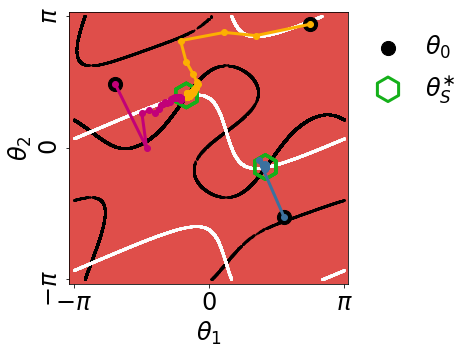Before doing so, we present an illustrative example in which several attracting critical points of the simultaneous gradient play dynamics are not differential Nash equilibria but are differential Stackelberg equilibria—meaning points $x\in X$ at which $-D_{2}^{2}f(x)>0$ , $\mathrm{spec}(J(x))\subset\mathbb{C}_{+}^{\circ}$ , and $D_{1}^{2}f(x)-D_{21}f(x)^{\top}(D_{2}^{2}f(x))^{-1}D_{21}f(x)>0$ .

Example 1 (Non-Nash Attractors are Stackelberg.).

Consider the zero-sum game defined by

f(x)=-e^{-0.01(x_{1}^{2}+x_{2}^{2})}((ax_{1}^{2}+x_{2})^{2}+(bx_{2}^{2}+x_{1})^{2}).

(5)

Let player $1$ be the leader who aims to minimize $f$ with respect to $x_{1}$ taking into consideration that player 2 (follower) aims to minimize $-f$ with respect to $x_{2}$ . In Fig. 1, we show the trajectories for various initializations for this game with $(a,b)=(0.15,0.25)$ ; it can be seen that for several initializations, simultaneous gradient play leads to non-Nash attractors which are differential Stackelberg equilibria.

Figure 1: Simultaneous gradient play is attracted to non-Nash differential Stackelberg equilibria: The game is given by the pair of cost functions

(f,-f)

where

f

is defined in (5) with

a=0.15

and

b=0.25

. There are two non-Nash attractors of simultaneous gradient play which are also differential Stackelberg equilibria.

We now proceed to provide necessary and sufficient conditions for the phenenom demonstrated in Example 1. Attracting critical points $x^{\ast}$ of the dynamics $\dot{x}=-\omega(x)$ that are not Nash equilibria are such that either $D_{1}^{2}f(x^{\ast})$ or $-D_{2}^{2}f(x^{\ast})$ are not positive definite. Without loss of generality, considering player 1 to be the leader, an attractor of the Stackelberg dynamics $\dot{x}=-\omega_{\mathcal{S}}(x)$ requires both $-D_{2}^{2}f(x^{\ast})$ and $D_{1}^{2}f(x^{\ast})-D_{21}f(x^{\ast})^{\top}(D_{2}^{2}f(x^{\ast}))^{-1}D_{21}f(x^{\ast})$ to be positive definite. Hence, if $-D_{2}^{2}f(x^{\ast})$ is not positive definite at a non-Nash attractor of $\dot{x}=-\omega(x)$ , then $x^{\ast}$ will also not be an attractor of $\dot{x}=-\omega_{\mathcal{S}}(x)$ . We focus on non-Nash attractors with $-D_{2}^{2}f(x^{\ast})>0$ and seek to determine when the Schur complement is positive definite, so that $x^{\ast}$ is an attractor of $\dot{x}=\omega_{\mathcal{S}}(x)$ .

In the following two propositions, we need some addition notion that is common across the two results. Let $x_{1}\in\mathbb{R}^{m}$ and $x_{2}\in\mathbb{R}^{n}$ . For a non-Nash attracting critical point $x^{\ast}$ , let $\mathrm{spec}(D_{1}^{2}f(x^{\ast}))=\{\mu_{j},\ j\in\{1,\ldots,m\}\}$ where

\mu_{1}\leq\cdots\leq\mu_{r}<0\leq\mu_{r+1}\leq\cdots\leq\mu_{m},

and let $\mathrm{spec}(-D_{2}^{2}f(x^{\ast}))=\{\lambda_{i},\ i\in\{1,\ldots,n\}\}$ where

\lambda_{1}\geq\cdots\geq\lambda_{n}>0,

and define $p=\dim(\ker(D_{1}^{2}f(x^{\ast})))$ .

Proposition 3 (Necessary conditions).

Consider a non-Nash attracting critical point $x^{\ast}$ of the gradient dynamics $\dot{x}=-\omega(x)$ such that $-D_{2}^{2}f(x^{\ast})>0$ . Given $\kappa>0$ such that $\|D_{21}f(x^{\ast})\|\leq\kappa$ , if $D_{1}^{2}f(x^{\ast})-D_{21}f(x^{\ast})^{\top}(D_{2}^{2}f(x^{\ast}))^{-1}D_{21}f(x^{\ast})>0$ , then $r\leq n$ and $\kappa^{2}\lambda_{i}+\mu_{i}>0$ for all $i\in\{1,\ldots,r-p\}$ .

Proposition 4 (Sufficient conditions).

Let $x^{\ast}$ be a non-Nash attracting critical point of the individual gradient dynamics $\dot{x}=-\omega(x)$ such that $D_{1}^{2}f(x^{\ast})$ and $-D_{2}^{2}f(x^{\ast})$ are Hermitian, and $-D_{2}^{2}f(x^{\ast})>0$ . Suppose that there exists a diagonal matrix (not necessarily positive) $\Sigma\in\mathbb{C}^{m\times n}$ with non-zero entries such that $D_{12}f(x^{\ast})=W_{1}\Sigma W_{2}^{\ast}$ where $W_{1}$ are the orthonormal eigenvectors of $D_{1}^{2}f(x^{\ast})$ and $W_{2}$ are orthonormal eigenvectors of $-D_{2}^{2}f(x^{\ast})$ . Given $\kappa>0$ such that $\|D_{21}f(x^{\ast})\|\leq\kappa$ , if $r\leq n$ and $\kappa^{2}\lambda_{i}+\mu_{i}>0$ for each $i\in\{1,\ldots,r-p\}$ , then $x^{\ast}$ is a differential Stackelberg equilibrium and an attractor of $\dot{x}=-\omega_{\mathcal{S}}(x)$ .

The proofs of the above results follow from some results linear algebra and are both in Appendix A.1. Essentially, this says that if $D_{1}^{2}f(x^{\ast})=W_{1}MW_{1}^{\ast}$ with $W_{1}W_{1}^{\ast}=I_{n\times n}$ and $M$ diagonal, and $-D_{2}^{2}f(x^{\ast})=W_{2}\Lambda W_{2}^{\ast}$ with $W_{2}W_{2}^{\ast}=I_{m\times m}$ and $\Lambda$ diagonal, then $D_{12}f(x^{\ast})$ can be written as $W_{1}\Sigma W_{2}^{\ast}$ for some diagonal matrix $\Sigma\in\mathbb{R}^{n\times m}$ (not necessarily positive). Note that since $\Sigma$ does not necessarily have positive values, $W_{1}\Sigma W_{2}^{\ast}$ is not the singular value decomposition of $D_{12}f(x^{\ast})$ . In turn, this means that the each eigenvector of $D_{1}^{2}f(x^{\ast})$ get mapped onto a single eigenvector of $-D_{2}^{2}f(x^{\ast})$ through the transformation $D_{12}f(x^{\ast})$ which describes how player 1’s variation $D_{1}f(x)$ changes as a function of player 2’s choice. With this structure for $D_{12}f(x^{\ast})$ , we can show that $D_{1}^{2}f(x^{\ast})-D_{21}f(x^{\ast})^{\top}(D_{2}^{2}f(x^{\ast}))^{-1}D_{21}f(x^{\ast})>0$ . If we remove the assumption that $\Sigma$ has non-zero entries, then the remaining assumptions are still sufficient to guarantee that

D_{1}^{2}f(x^{\ast})-D_{21}f(x^{\ast})^{\top}(D_{2}^{2}f(x^{\ast}))^{-1}D_{21}f(x^{\ast})\geq 0.

This means that $x^{\ast}$ does not satisfy the conditions for a differential Stackelberg, however, the point does satisfy necessary conditions for a local Stackelberg equilibrium and the point is a marginally stable attractor of the dynamics.

While the results depend on conditions that are difficult to check a priori without knowledge of $x^{\ast}$ , certain classes of games for which these conditions hold everywhere and not just at the equilibrium can be constructed. For instance, alternative conditions can be given: if the function $f$ which defines the zero-sum game is such that it is concave in $x_{2}$ and there exists a $K$ such that

D_{12}f(x)=KD_{2}^{2}f(x)

where $\sup_{x}\|D_{12}f(x)\|\leq\kappa<\infty$ ³³ 3 Functions such that derivative of $f$ is Lipschitz will satisfy this condition. and $K=W_{1}\Sigma W_{2}^{\ast}$ with $\Sigma$ again a (not necessarily positive) diagonal matrix, then the results of Proposition 4 hold. From a control point of view, one can think about the leader’s update as having a feedback term with the follower’s input. On the other hand, the results are useful for the synthesis of games, such as in reward shaping or incentive design, where the goal is to drive agents to particular desirable behavior.

We remark that the fact that the eigenvalues of $J(x^{\ast})$ are in the open-right-half complex plane is not used in proving this result. We believe that further investigation could lead to a less restrictive sufficient condition. Empirically, by randomly generating the different block matrices, it is quite difficult to find examples such that $J(x^{\ast})$ has positive eigenvalues, $-D_{2}^{2}f(x^{\ast})>0$ , and the Schur complement $D_{1}^{2}f(x^{\ast})-D_{21}f(x^{\ast})^{\top}(D_{2}^{2}f(x^{\ast}))^{-1}D_{21}f(x^{\ast})$ is not positive definite. In fact, for games on scalar action spaces, it turns out that non-Nash attracting critical points of the simultaneous gradient play dynamics at which $-D_{2}^{2}f(x^{\ast})>0$ must be differential Stackelberg equilibria and attractors of the Stackelberg limiting dynamics.

Corollary 1.

Consider a zero-sum game $(f,-f)$ defined by a sufficiently smooth cost function $f:\mathbb{R}^{2}\rightarrow\mathbb{R}$ such that the action space is $X=\mathbb{R}\times\mathbb{R}$ and player 1 is deemed the leader and player 2 the follower. Then, any non-Nash attracting critical point of $\dot{x}=-\omega(x)$ at which $-D_{2}^{2}f(x)>0$ is a differential Stackelberg equilibrium and an attractor of $\dot{x}=-\omega_{\mathcal{S}}(x)$ .

Proof. Consider a sufficiently smooth zero-sum game $(f,-f)$ on continuous strategy spaces defined by the cost function $f:\mathbb{R}^{2}\rightarrow\mathbb{R}$ . Suppose $x^{\ast}$ is an attracting critical point of the dynamics $\dot{x}=-\omega(x)$ at which $-D_{2}^{2}f(x^{\ast})>0$ and $D_{1}^{2}f(x^{\ast})<0$ so that it is not a Nash equilibria. The Jacobian of the dynamics at a stable critical point is

J(x^{\ast})=\begin{bmatrix}D_{1}^{2}f(x^{\ast})&D_{12}f(x^{\ast})\\ -D_{21}f(x^{\ast})&-D_{2}^{2}f(x^{\ast})\end{bmatrix}>0.

The fact that the real components of the eigenvalues of the Jacobian are positive implies that $D_{12}f(x^{\ast})D_{21}f(x^{\ast})>D_{1}^{2}f(x^{\ast})D_{2}^{2}f(x^{\ast})$ and $D_{1}^{2}f(x^{\ast})>D_{2}^{2}f(x^{\ast})$ since the determinant and the trace of the Jacobian must be positive. Using this information, it directly follows that the Schur complement of $J(x^{\ast})$ is positive definite:

D_{1}^{2}f(x^{\ast})-D_{12}f(x^{\ast})(D_{2}^{2}f(x^{\ast}))^{-1}D_{21}f(x^{\ast})>0.

As a result, $x^{\ast}$ is a differential Stackelberg equilibrium and an attractor of $\dot{x}=-\omega_{\mathcal{S}}(x)$ since the Schur complement of $J(x^{\ast})$ is the derivative $D^{2}f(x^{\ast})$ and $-D_{2}^{2}f(x)>0$ was given.
We suspect that using the notion of quadratic numerical range [58], which is a super set of the spectrum of a block operator matrix, along with the fact that the Jacobian of the simultaneous gradient play dynamics has its spectrum in the open right-half complex plane, may lead to an extension of the result to arbitrary dimensions.

The results of Propositions 3 and 4, Corollary 1, and Example 1 imply that some of the non-Nash attractors of $\dot{x}=-\omega(x)$ are in fact Stackelberg equilibria. This is a meaningful insight since recent works have proposed schemes to avoid non-Nash attractors of the dynamics as they have been classified or viewed as lacking game-theoretic meaning [37]. Moreover, some recent empirical results show that a number of successful approaches to training GANs are not converging to Nash equilibria, but rather to non-Nash attractors of the dynamics [8]. It would be interesting to characterize whether or not the attractors satisfy the conditions we propose, and if such conditions could provide insights into how to improve GAN training. It also further suggests that the Stackelberg equilibria may be a suitable solution concept for GANs.

One of the common assumptions in some of the recent GANs literature is that the discriminator network is zero in a neighborhood of an equilibrium parameter configuration (see, e.g., [43, 44, 41]). This assumption limits the theory to the ‘realizable’ case; the work by [43] provides relaxed assumptions for the non-realizable case. In both cases, the Jacobian for the dynamics $\dot{x}=-\omega(x)$ is such that $D_{1}^{2}f(x^{\ast})=0$ .

Proposition 5.

Consider a GAN satisfying the realizable assumption—that is, the discriminator network is zero in a neighborhood of any equilibrium. Then, an attracting critical point for the simultaneous gradient dynamics $\dot{x}=-\omega(x)$ at which $-D_{2}^{2}f$ is positive semi-definite satisfies necessary conditions for a local Stackelberg equilibrium, and it will be a marginally stable point of the Stackelberg dynamics $\dot{x}=-\omega_{\mathcal{S}}(x)$ .

Proof. Consider an attracting critical point $x$ of $\dot{x}=-\omega(x)$ such that $-D_{2}^{2}f(x^{\ast})\geq 0$ . Note that the realizable assumption implies that the Jacobian of $\omega$ is

J(x^{\ast})=\begin{bmatrix}0&D_{12}f(x^{\ast})\\ -D_{21}f(x^{\ast})&-D_{2}^{2}f(x^{\ast})\end{bmatrix}

(see, e.g., [43]). Hence, since $-D_{2}^{2}f(x^{\ast})\geq 0$ ,

-D_{21}^{\top}f(x^{\ast})(D_{2}^{2}f)^{-1}(x^{\ast})D_{21}f(x^{\ast})\geq 0.

Since $x^{\ast}$ is an attractor, $D_{1}f(x^{\ast})=0$ and $D_{2}f(x^{\ast})=0$ so that

Df(x^{\ast})=D_{1}f(x^{\ast})+D_{2}f(x^{\ast})(D_{2}^{2}f)^{-1}(x^{\ast})D_{21}f(x^{\ast})=0

Consequently, the necessary conditions for a local Stackelberg equilibrium are satisfied. Moreover, since both $-D_{2}^{2}f(x^{\ast})\geq 0$ and the Schur complement $-D_{21}^{\top}f(x^{\ast})(D_{2}^{2})^{-1}f(x^{\ast})D_{21}f(x^{\ast})\geq 0$ , the Jacobian of $\omega_{\mathcal{S}}$ is positive semi-definite so that the point $x^{\ast}$ is marginally stable.

Now, simply satisfying the necessary conditions is not enough to guarantee that attractors of the simultaneous play gradient dynamics will be a local Stackelberg equilibrium. We can state sufficient conditions by examining Proposition 4.

Proposition 6.

Consider a GAN satisfying the realizable assumption—that is, the discriminator network is zero in a neighborhood of any equilibrium—and an attractor for the simultaneous gradient dynamics $\dot{x}=-\omega(x)$ at which $-D_{2}^{2}f$ is positive definite. Suppose that there exists a diagonal matrix $\Sigma$ with non-zero entries such that $D_{12}f(x^{\ast})=\Sigma W$ where $W$ are the orthonormal eigenvectors of $-D_{2}^{2}f(x^{\ast})$ . Then, $x^{\ast}$ is a differential Stackelberg equilibrium and an attractor of $\dot{x}=-\omega_{\mathcal{S}}(x)$ .

The proof follows directly from Proposition 4 and Proposition 5. It is not directly clear how restrictive these sufficient conditions are for GANs. We leave this for future inquiry.

2.2.2 Connections to Opponent Shaping

Beyond the work in zero-sum games and applications to GANs, there has also been recent work, which we will refer to as ‘opponent shaping’, where one or more players takes into account its opponents’ response to their action [33, 21, 60]. The initial work of Foerster et al. 2018 bears the most resemblance to the learning algorithms studied in this paper. The update rule (LOLA) considered there (in the deterministic setting with constant stepsizes) takes the following form:

	$\displaystyle x_{1}^{+}$	$\displaystyle=x_{1}-\gamma_{1}(D_{1}f_{1}(x)-\gamma_{2}D_{2}f_{1}(x)D_{21}f_{2}(x))$
	$\displaystyle x_{2}^{+}$	$\displaystyle=x_{2}-\gamma_{2}D_{2}f_{2}(x)$

The attractors of these dynamics are not necessarily Nash equilibria nor are they Stackelberg equilibria as can be seen by looking at the critical points of the dynamics. Indeed, the LOLA dynamics lead only to Nash or non-Nash stable attractors of the limiting dynamics. The effect of the additional ‘look-ahead’ term is simply that it changes the vector field and region of attraction for stable critical points. In the zero-sum case, however, the critical points of the above are the same as those of simultaneous play individual gradient updates, yet the Jacobian is not the same and it is still possible to converge to a non-Nash attractor.

With a few modifications, the above update rule can be massaged into a form which more closely resembles the hierarchical learning rules we study in this paper. In particular, if instead of $\gamma_{2}$ , player 2 employed a Newton stepsize of $(D_{2}^{2}f_{2})^{-1}$ , then the update would look like

	$\displaystyle x_{1}^{+}$	$\displaystyle=x_{1}-\gamma_{1}(D_{1}f_{1}(x)-D_{2}f_{1}(x)(D_{2}^{2}f_{2}(x))^{-1}D_{21}f_{2}(x))$
	$\displaystyle x_{2}^{+}$	$\displaystyle=x_{2}-\gamma_{2}D_{2}f_{2}(x)$

which resembles a deterministic version of (1). The critical points of this update coincide with the critical points of a Stackelberg game $(f_{1},f_{2})$ . With appropriately chosen stepsizes and with an initialization in a region on which the implicit map, which defines the $-(D_{2}^{2}f_{2}(x))^{-1}D_{21}f_{2}(x)$ component of the update, is well-defined uniformly in $x_{1}$ , the above dynamics will converge to Stackelberg equilibria. In this paper, we provide an in-depth convergence analysis and for the stochastic setting⁴⁴ 4 In [21], the authors do not provide convergence analysis; they do in their extension, yet only for constant and uniform stepsizes and for a learning rule that is different than the one studied in this paper as all players are conjecturing about the behavior of their opponents. This distinguishes the present work from their setting. of the above update.

2.2.3 Comparing Nash and Stackelberg Equilibrium Cost

We have alluded to the idea that the ability to act first gives the leader a distinct advantage over the follower in a hierarchical game. We now formalize this statement with a known result that compares the cost of the leader at Nash and Stackelberg equilibrium.

Proposition 7.

([4, Proposition 4.4]). Consider an arbitrary sufficiently smooth two-player general-sum game $(f_{1},f_{2})$ on continuous strategy spaces. Let $f_{1}^{\mathcal{N}}$ denote the infimum of all Nash equilibrium costs for player 1 and $f_{1}^{\mathcal{S}}$ denote an arbitrary Stackelberg equilibrium cost for player 1. Then, if $\mathcal{R}(x_{1})$ is a singleton for every $x_{1}\in X_{1}$ , $f_{1}^{\mathcal{S}}\leq f_{1}^{\mathcal{N}}$ .

This result says that the leader never favors the simultaneous play game over the hierarchical play game in two-player general-sum games with unique follower responses. On the other hand, the follower may or may not prefer the simultaneous play game over the hierarchical play game.

The fact that under certain conditions the leader can obtain lower cost under a Stackelberg equilibrium compared to any of the Nash equilibrium may provide further explanation for the success of the methods in [42]. Commonly, the discriminator can overpower the generator when training a GAN [42] and giving the generator an advantage may mitigate this problem. In the context of multi-agent learning, the advantage of the leader in hierarchical games leads to the question of how the roles of each player in a game are decided. While we do not focus on this question, it is worth noting that when each player mutually benefits from the leadership of a player the solution is called concurrent and when each player prefers to be the leader the solution is called non-concurrent. We believe that exploring classes of games in which each solution concept arises is an interesting direction of future work.

3 Convergence Analysis

Following the preceding discussion, consider the learning rule for each player to be given by

x_{i,k+1}=x_{i,k}-\gamma_{i,k}(\omega_{\mathcal{S},i}(x_{k})+w_{i,k+1}),

(6)

where recall that $\omega_{\mathcal{S}}=(Df_{1}(x),D_{2}f_{2}(x))$ . Moreover, for each $i\in\mathcal{I}$ , $\{\gamma_{i,k}\}$ is the sequence of learning rates and $\{w_{i,k}\}$ is the noise process for player $i$ . As before, suppose player 1 is the leader and conjectures that player 2 updates its action $x_{2}$ in each round via $r(x_{1})$ . This setting captures the scenario in which players do not have oracle access to their gradients, but do have an unbiased estimator. As an example, players could be performing policy gradient reinforcement learning or alternative gradient-based learning schemes. Let $\dim(X_{i})=d_{i}$ for each $i\in\mathcal{I}$ and $d=d_{1}+d_{2}$ .

Assumption 1.

The following hold:

A1a.

The maps $Df_{1}:\mathbb{R}^{d}\rightarrow\mathbb{R}^{d_{1}}$ , $D_{2}f_{2}:\mathbb{R}^{d}\rightarrow\mathbb{R}^{d_{2}}$ are $L_{1}$ , $L_{2}$ Lipschitz, and $\|Df_{1}\|\leq M_{1}<\infty$ .
A1b.

For each $i\in\mathcal{I}$ , the learning rates satisfy $\sum_{k}\gamma_{i,k}=\infty$ , $\sum_{k}\gamma_{i,k}^{2}<\infty$ .
A1c.

The noise processes $\{w_{i,k}\}$ are zero mean, martingale difference sequences. That is, given the filtration $\mathcal{F}_{k}=\sigma(x_{s},w_{1,s},w_{2,s},\ s\leq k)$ , $\{w_{i,k}\}_{i\in\mathcal{I}}$ are conditionally independent, $\mathbb{E}[w_{i,k+1}|\ \mathcal{F}_{k}]=0$ a.s., and $\mathbb{E}[\|w_{i,k+1}\||\ \mathcal{F}_{k}]\leq c_{i}(1+\|x_{k}\|)$ a.s. for some constants $c_{i}\geq 0$ , $i\in\mathcal{I}$ .

Before diving into the convergence analysis, we need some machinery from dynamical systems theory. Consider the dynamics from (6) written as a continuous time combined system $\dot{\xi_{t}}=F(\xi_{t})$ where $\xi_{t}(z)=\xi(t,z)$ is a continuous map and $\xi=\{\xi_{t}\}_{t\in\mathbb{R}}$ is the flow of $F$ . A set $A$ is said to be invariant under the flow $\xi$ if for all $t\in\mathbb{R}$ , $\xi_{t}(A)\subset A$ , in which case $\xi|A$ denotes the semi-flow. A point $x$ is an equilibrium if $\xi_{t}(x)=x$ for all $t$ and, of course, when $\xi$ is induced by $F$ , equilibria coincide with critical points of $F$ . Let $X$ be a topological metric space with metric $\rho$ , an example being $X=\mathbb{R}^{d}$ endowed with the Euclidean distance.

Definition 5.

A nonempty invariant set $A\subset X$ for $\xi$ is said to be internally chain transitive if for any $a,b\in A$ and $\delta>0$ , $T>0$ , there exists a finite sequence $\{x_{1}=a,x_{2},\ldots,x_{k-1},x_{k}=b;t_{1},\ldots,t_{k-1}\}$ with $x_{i}\in A$ and $t_{i}\geq T$ , $1\leq i\leq k-1$ , such that $\rho(\xi_{t_{i}}(x_{i}),x_{i+1})<\delta$ , $\forall 1\leq i\leq k-1$ .

3.1 Learning Stackelberg Solutions for the Leader

Suppose that the leader (player 1) operates under the assumption that the follower (player 2) is playing a local optimum in each round. That is, given $x_{1,k}$ , $x_{2,k+1}\in\arg\min_{x_{2}}f_{2}(x_{1,k},x_{2})$ for which $D_{2}f_{2}(x_{1,k},x_{2})=0$ is a first-order local optimality condition. If, for a given $(x_{1},x_{2})\in X_{1}\times X_{2}$ , $D_{2}^{2}f_{2}(x_{1},x_{2})$ is invertible and $D_{2}f_{2}(x_{1},x_{2})=0$ , then the implicit function theorem implies that there exists neighborhoods $U\subset X_{1}$ and $V\subset X_{2}$ and a smooth map $r:U\rightarrow V$ such that $r(x_{1})=x_{2}$ .

Assumption 2.

For every $x_{1}$ , $\dot{x}_{2}=-D_{2}f_{2}(x_{1},x_{2})$ has a globally asymptotically stable equilibrium $r(x_{1})$ uniformly in $x_{1}$ and $r:\mathbb{R}^{d_{1}}\rightarrow\mathbb{R}^{d_{2}}$ is $L_{r}$ –Lipschitz.

Consider the leader’s learning rule

x_{1,k+1}=x_{1,k}-\gamma_{1,k}(Df_{1}(x_{1,k},x_{2,k})+w_{1,k+1})

(7)

where $x_{2,k}$ is defined via the map $r_{2}$ defined implicitly in a neighborhood of $(x_{1,k},x_{2,k})$ .

Proposition 8.

Suppose that for each $x\in X$ , $D_{2}^{2}f_{2}$ is non-degenerate and Assumption 1 holds for $i=1$ . Then, $x_{1,k}$ converges almost surely to an (possibly sample path dependent) equilibrium point $x_{1}^{\ast}$ which is a local Stackelberg solution for the leader. Moreover, if Assumption 1 holds for $i=2$ and Assumption 2 holds, then $x_{2,k}\rightarrow x_{2}^{\ast}=r(x_{1}^{\ast})$ so that $(x_{1}^{\ast},x_{2}^{\ast})$ is a differential Stackelberg equilibrium.

Proof. This proof follows primarily from using known stochastic approximation results. The update rule in (7) is a stochastic approximation of $\dot{x}_{1}=-Df_{1}(x_{1},x_{2})$ and consequently is expected to track this ODE asymptotically. The main idea behind the analysis is to construct a continuous interpolated trajectory $\bar{x}(t)$ for $t\geq 0$ and show it asymptotically almost surely approaches the solution set to the ODE. Under Assumptions 1–3, results from [11, §2.1] imply that the sequence generated from (7) converges almost surely to a compact internally chain transitive set of $\dot{x}_{1}=-Df_{1}(x_{1},x_{2})$ . Furthermore, it can be observed that the only internally chain transitive invariant sets of the dynamics are differential Stackelberg equilibria since at any stable attractor of the dynamics $D^{2}f_{1}(x_{1},r(x_{1}))>0$ and from assumption $D_{2}^{2}f_{2}(x_{1},r(x_{1}))>0$ . Finally, from [11, §2.2], we can conclude that the update from (7) almost surely converges to a possibly sample path dependent equilibrium point since the only internally chain transitive invariant sets for $\dot{x}_{1}=-Df_{1}(x_{1},x_{2})$ are equilibria. The final claim that $x_{2,k}\to r(x_{1}^{\ast})$ is guaranteed since $r$ is Lipschitz and $x_{1,k}\to x_{1}^{\ast}$ .

The above result can be stated with a relaxed version of Assumption 2.

Corollary 2.

Given a differential Stackelberg equilibrium $x^{\ast}=(x_{1}^{\ast},x_{2}^{\ast})$ , let $B_{q}(x^{\ast})=B_{q_{1}}(x_{1}^{\ast})\times B_{q_{2}}(x_{2}^{\ast})$ for some $q_{1},q_{2}>0$ on which $D_{2}^{2}f_{2}$ is non-degenerate. Suppose that Assumption 1 holds for $i=1$ and that $x_{1,0}\in B_{q_{1}}(x_{1}^{\ast})$ . Then, $x_{1,k}$ converges almost surely to $x_{1}^{\ast}$ . Moreover, if Assumption 1 holds for $i=2$ , $r(x_{1})$ is a locally asymptotically stable equilibrium uniformly in $x_{1}$ on the ball $B_{q_{2}}(x_{2}^{\ast})$ , and $x_{2,0}\in B_{q_{2}}(x_{2}^{\ast})$ , then $x_{2,k}\rightarrow x_{2}^{\ast}=r(x_{1}^{\ast})$ .

The proof follows the same arguments as the proof of Proposition 8.

3.2 Learning Stackelberg Equilibria: Two-Timescale Analysis

Now, let us consider the case where the leader again operates under the assumption that the follower is playing (locally) optimally at each round so that the belief is $D_{2}f_{2}(x_{1,k},x_{2,k})=0$ , but the follower is actually performing the update $x_{2,k+1}=x_{2,k}+g_{2}(x_{1,k},x_{2,k})$ where $g_{2}\equiv-\gamma_{2,k}\mathbb{E}[D_{2}f_{2}]$ . The learning dynamics in this setting are then

	$\displaystyle x_{1,k+1}$	$\displaystyle=x_{1,k}-\gamma_{1,k}(Df_{1}(x_{k})+w_{1,k+1})$		(8)
	$\displaystyle x_{2,k+1}$	$\displaystyle=x_{2,k}-\gamma_{2,k}(D_{2}f_{2}(x_{k})+w_{2,k+1})$		(9)

where $Df_{1}(x)=D_{1}f_{1}(x)+D_{2}f_{1}(x)Dr(x_{1})$ . Suppose that $\gamma_{1,k}\rightarrow 0$ faster than $\gamma_{2,k}$ so that in the limit $\tau\rightarrow 0$ , the above approximates the singularly perturbed system defined by

\begin{array}[]{lcl}\dot{x}_{1}(t)&=&-\tau Df_{1}(x_{1}(t),x_{2}(t))\\ \dot{x}_{2}(t)&=&-D_{2}f_{2}(x_{1}(t),x_{2}(t))\end{array}

(10)

The learning rates can be seen as stepsizes in a discretization scheme for solving the above dynamics. The condition that $\gamma_{1,k}=o(\gamma_{2,k})$ induces a timescale separation in which $x_{2}$ evolves on a faster timescale than $x_{1}$ . That is, the fast transient player is the follower and the slow component is the leader since $\lim_{k\rightarrow\infty}\gamma_{1,k}/\gamma_{2,k}=0$ implies that from the perspective of the follower, $x_{1}$ appears quasi-static and from the perspective of the leader, $x_{2}$ appears to have equilibriated, meaning $D_{2}f_{2}(x_{1},x_{2})=0$ given $x_{1}$ . From this point of view, the learning dynamics (8)–(9) approximate the dynamics in the preceding section. Moreover, stable attractors of the dynamics are such that the leader is at a local optima for $f_{1}$ , not just along its coordinate axis but in both coordinates $(x_{1},x_{2})$ constrained to the manifold $r(x_{1})$ ; this is to make a distinction between differential Nash equilibria in agents are at local optima aligned with their individual coordinate axes.

3.2.1 Asymptotic Almost Sure Convergence

The following two results are fairly classical results in stochastic approximation. They are leveraged here to making conclusions about convergence to Stackelberg equilibria in hierarchical learning settings.

While we do not need the following assumption for all the results in this section, it is required for asymptotic convergence of the two-timescale process in (8)–(9).

Assumption 3.

The dynamics $\dot{x}_{1}=-Df_{1}(x_{1},r(x_{1}))$ have a globally asymptotically stable equilibrium.

Under Assumption 1–3, and the assumption that $\gamma_{1,k}=o(\gamma_{2,k})$ , classical results imply that the dynamics (8)–(9) converge almost surely to a compact internally chain transitive set $\mathcal{T}$ of (10); see, e.g., [11, §6.1-2], [10, §3.3]. Furthermore, it is straightforward to see that stable differential Nash equilibria are internally chain transitive sets since they are stable attractors of the dynamics $\dot{\xi}_{t}=F(\xi_{t})$ from (10).

Remark 3.

There are two important points to remark on at this juncture. First, the flow of the dynamics (10) is not necessarily a gradient flow, meaning that the dynamics may admit non-equilibrium attractors such as periodic orbits. The dynamics correspond to a gradient vector field if and only if $D_{2}(Df_{1})\equiv D_{12}f_{2}$ , meaning when the dynamics admit a potential function. Equilibria may also not be isolated unless the Jacobian of $\omega_{\mathcal{S}}$ , say $J_{\mathcal{S}}$ , is non-degenerate at the points. Second, except in the case of zero-sum settings in which $(f_{1},f_{2})=(f,-f)$ , non-Stackelberg locally asymptotically stable equilibria are attractors. That is, convergence does not imply that the players have settled on a Stackelberg equilibrium, and this can occur even if the dynamics admit a potential.

Let $t_{k}=\sum_{l=0}^{k-1}\gamma_{1,l}$ be the (continuous) time accumulated after $k$ samples of the slow component $x_{1}$ . Define $\xi_{1,s}(t)$ to be the flow of $\dot{x}_{1}=-Df_{1}(x_{1}(t),r(x_{1}(t)))$ starting at time $s$ from intialization $x_{s}$ .

Proposition 9.

Suppose that Assumptions 1 and 2 hold. Then, conditioning on the event $\{\sup_{k}\sum_{i}\|x_{i,k}\|^{2}<\infty\}$ , for any integer $K>0$ , $\lim_{k\rightarrow\infty}\sup_{0\leq h\leq K}\|x_{1,k+h}-\xi_{1,t_{k}}(t_{k+h})\|_{2}=0$ almost surely.

Proof. The proof follows standard arguments in stochastic approximation. We simply provide a sketch here to give some intuition. First, we show that conditioned on the event $\{\sup_{k}\sum_{i}\|x_{1,k}\|^{2}<\infty\}$ , $(x_{1,k},x_{2,k})\rightarrow\{(x_{1},r(x_{1}))|\ x_{1}\in\mathbb{R}^{d_{1}}\}$ almost surely. Let $\zeta_{k}=\frac{\gamma_{1,k}}{\gamma_{2,k}}(Df_{1}(x_{k})+w_{1,k+1})$ . Hence the leader’s sample path is generated by $x_{1,k+1}=x_{1,k}-\gamma_{2,k}\zeta_{k}$ which tracks $\dot{x}_{1}=0$ since $\zeta_{k}=o(1)$ so that it is asymptotically negligible. In particular, $(x_{1,k},x_{2,k})$ tracks $(\dot{x}_{1}=0,\dot{x}_{2}=-D_{2}f_{2}(x_{1},x_{2}))$ . That is, on intervals $[\hat{t}_{j},\hat{t}_{j+1}]$ where $\hat{t}_{j}=\sum_{l=0}^{j-1}\gamma_{2,l}$ , the norm difference between interpolated trajectories of the sample paths and the trajectories of $(\dot{x}_{1}=0,\dot{x}_{2}=-D_{2}f_{2}(x_{1},x_{2}))$ vanishes a.s. as $k\rightarrow\infty$ . Since the leader is tracking $\dot{x}_{1}=0$ , the follower can be viewed as tracking $\dot{x}_{2}(t)=-D_{2}f_{2}(x_{1},x_{2}(t))$ . Then applying Lemma 4 provided in Appendix A, $\lim_{k\rightarrow 0}\|x_{2,k}-r(x_{1,k})\|\rightarrow 0$ almost surely.

Now, by Assumption 1, $Df_{1}$ is Lipschitz and bounded (in fact, independent of A1a., since $Df_{1}\in C^{q}$ , $q\geq 2$ , it is locally Lipschtiz and, on the event $\{\sup_{k}\sum_{i}\|x_{i,k}\|_{2}<\infty\}$ , it is bounded). In turn, it induces a continuous globally integrable vector field, and therefore satisfies the assumptions of Benaïm 1999. Moreover, under Assumptions A1b. and A1c., the assumptions of Benaïm 1999 are satisfied, which gives the desired result.

Corollary 3.

Under Assumption 3 and the assumptions of Proposition 9, $(x_{1,k},x_{2,k})\rightarrow(x_{1}^{\ast},r(x_{1}^{\ast}))$ almost surely conditioned on the event $\textstyle\{\sup_{k}\sum_{i}\|x_{i,k}\|^{2}<\infty\}$ . That is, the learning dynamics (8)–(9) converge to stable attractors of (10), the set of which includes the stable differential Stackelberg equilibria.

Proof. Continuing with the conclusion of the proof of Proposition 9, on intervals $[t_{k},t_{k+1}]$ the norm difference between interpolates of the sample path and the trajectories of $\dot{x}_{1}=-Df_{1}(x_{1},r(x_{1}))$ vanish asymptotically; applying Lemma 4 (Appendix A) gives the result.
Leveraging the results in Section 2.2.1, the convergence guarantees are stronger since in zero-sum settings all attractors are Stackelberg; this contrasts with the Nash equilibrium concept.

Corollary 4.

Consider a zero-sum setting $(f,-f)$ . Under the assumptions of Proposition 9 and Assumption 3, conditioning on the event $\{\sup_{k}\sum_{i}\|x_{i,k}\|^{2}<\infty\}$ , the learning dynamics (8)–(9) converge to a differential Stackelberg equilibria almost surely.

The proof of this corollary follows the above analysis and invokes Proposition 1. As with Corollary 2, we can relax Assumption 2 and 3 to local asymptomatic stability assumptions and obtain similarity convergence guarantees.

Corollary 5.

Given a differential Stackelberg equilibrium $x^{\ast}=(x_{1}^{\ast},x_{2}^{\ast})$ where $x_{2}^{\ast}=r(x_{1}^{\ast})$ , let $B_{q}(x^{\ast})=B_{q_{1}}(x_{1}^{\ast})\times B_{q_{2}}(x_{2}^{\ast})$ for some $q_{1},q_{2}>0$ on which $D_{2}^{2}f_{2}$ is non-degenerate. Suppose that Assumption 1 holds for each player, $r(x_{1})$ is a locally asymptotically stable attractor uniformly in $x_{1}$ on the ball $B_{q_{2}}(x_{2}^{\ast})$ for the dynamics $\dot{x}_{2}=-D_{2}f_{2}(x)$ , and there exists a locally asymptotically stable attractor on $B_{q_{1}}(x_{1})$ for the dynamics $\dot{x}_{1}=-Df_{1}(x_{1},r(x_{1}))$ . Then, given an initialization $x_{1,0}\in B_{q_{1}}(x_{1}^{\ast})$ and $x_{2,0}\in B_{q_{2}}(x_{2}^{\ast})$ , it follows that $(x_{1,k},x_{2,k})\rightarrow(x_{1}^{\ast},x_{2}^{\ast})$ almost surely.

3.2.2 Finite-Time High-Probability Guarantees

While asymptotic guarantees of the proceeding section are useful, high-probability finite-time guarantees can be leveraged more directly in analysis and synthesis, e.g., of mechanisms to coordinate otherwise autonomous agents. In this section, we aim to provide concentration bounds for the purpose of deriving convergence rate and error bounds in support of this objective. The results in this section follow the very recent work by Borkar and Pattathil 2018. We highlight key differences and, in particular, where the analysis may lead to insights relevant for learning in hierarchical decision problems between non-cooperative agents.

Consider a locally asymptotically stable differential Stackelberg equilibrium $x^{\ast}=(x_{1}^{\ast},r(x_{1}^{\ast}))\in X$ and let $B_{q_{0}}(x^{\ast})$ be an ${q}_{0}>0$ radius ball around $x^{\ast}$ contained in the region of attraction. Stability implies that the Jacobian $J_{\mathcal{S}}(x_{1}^{\ast},r(x_{1}^{\ast}))$ is positive definite and by the converse Lyapunov theorem [55, Chap. 5] there exists local Lyapunov functions for the dynamics $\dot{x}_{1}(t)=-\tau Df_{1}(x_{1}(t),r(x_{1}(t)))$ and for the dynamics $\dot{x}_{2}(t)=-D_{2}f_{2}(x_{1},x_{2}(t))$ , for each fixed $x_{1}$ . In particular, there exists a local Lyapunov function $V\in C^{1}(\mathbb{R}^{d_{1}})$ with $\lim_{\|x_{1}\|\uparrow\infty}V(x_{1})=\infty$ , and $\langle\nabla V(x_{1}),Df_{1}(x_{1},r(x_{1}))\rangle<0$ for $x_{1}\neq x_{1}^{\ast}$ . For $q>0$ , let $V^{q}=\{x\in\text{dom}(V):\ V(x)\leq q\}$ . Then, there is also $q>q_{0}>0$ and $\epsilon_{0}>0$ such that for $\epsilon<\epsilon_{0}$ , $\{x_{1}\in\mathbb{R}^{d_{1}}|\ \|x_{1}-x_{1}^{\ast}\|\leq\epsilon\}\subseteq V^{q_{0}}\subset\mathcal{N}_{\epsilon_{0}}(V^{q_{0}})\subseteq V^{q}\subset\text{dom}(V)$ where $\mathcal{N}_{\epsilon_{0}}(V^{q_{0}})=\{x\in\mathbb{R}^{d_{1}}|\ \exists x^{\prime}\in V^{q_{0}}\ \text{s.t.}\|x^{\prime}-x\|\leq\epsilon_{0}\}$ . An analogously defined $\tilde{V}$ exists for the dynamics $\dot{x}_{2}$ for each fixed $x_{1}$ .

For now, fix $n_{0}$ sufficiently large; we specify the values of $n_{0}$ for which the theory holds before the statement of Theorem 1. Define the event $\mathcal{E}_{n}=\{\bar{x}_{2}(t)\in V^{q}\ \forall t\in[\tilde{t}_{n_{0}},\tilde{t}_{n}]\}$ where $\bar{x}_{2}(t)=x_{2,k}+\frac{t-\tilde{t}_{k}}{\gamma_{2,k}}(x_{2,k+1}-x_{2,k})$ are linear interpolates—i.e., asymptotic pseudo-trajectories—defined for $t\in(\tilde{t}_{k},\tilde{t}_{k+1})$ with $\tilde{t}_{k+1}=\tilde{t}_{k}+\gamma_{2,k}$ and $\tilde{t}_{0}=0$ .

The basic idea of the proof is to leverage Alekseev’s formula (Thm. 3, Appendix A) to bound the difference between the asymptotic pseudo-trajectories and the flow of the corresponding limiting differential equation on each continuous time interval between each of the successive iterates $k$ and $k+1$ by sequences of constants that decay asymptotically. Then, a union bound is used over all time intervals after defined for $n\geq n_{0}$ in order to construct a concentration bound. This is done first for the follower, showing that $x_{2,k}$ tracks the leader’s ’conjecture’ or belief $r(x_{1,k})$ about the follower’s reaction, and then for the leader.

Following Borkar and Pattathil 2018, we can express the linear interpolates for any $n\geq n_{0}$ as $\bar{x}_{2}(\tilde{t}_{n+1})\textstyle=\bar{x}_{2}(\tilde{t}_{n_{0}})-\sum_{k=n_{0}}^{n}\gamma_{2,k}(D_{2}f_{2}(x_{k})+w_{2,k+1})$ where $\textstyle\gamma_{2,k}D_{2}f_{2}(x_{k})=\int_{\tilde{t}_{k}}^{\tilde{t}_{k+1}}D_{2}f_{2}(x_{1,k},\bar{x}_{2}(\tilde{t}_{k}))\ ds$ and similarly for the $w_{2,k+1}$ term. Adding and subtracting $\int_{\tilde{t}_{n_{0}}}^{\tilde{t}_{n+1}}D_{2}f_{2}(x_{1}(s),\bar{x}_{2}(s))\ ds$ , Alekseev’s formula can be applied to get

\displaystyle\bar{x}_{2}(t)

\displaystyle=x_{2}(t)+\Phi_{2}(t,s,x_{1}(\tilde{t}_{n_{0}}),\bar{x}_{2}(\tilde{t}_{n_{0}}))(\bar{x}_{2}(\tilde{t}_{n_{0}})\textstyle-x_{2}(\tilde{t}_{n_{0}}))+\int_{\tilde{t}_{n_{0}}}^{t}\Phi_{2}(t,s,x_{1}(s),\bar{x}_{2}(s))\zeta_{2}(s)\ ds

where $x_{1}(t)\equiv x_{1}$ is constant (since $\dot{x}_{1}=0$ ), $x_{2}(t)=r(x_{1})$ , and

\zeta_{2}(s)=-D_{2}f_{2}(x_{1}(\tilde{t}_{k}),\bar{x}_{2}(\tilde{t}_{k}))+D_{2}f_{2}(x_{1}(s),\bar{x}_{2}(s))+w_{2,k+1}.

In addition, for $t\geq s$ , $\Phi_{2}(\cdot)$ satisfies linear system

\dot{\Phi}_{2}(t,s,x_{0})=J_{2}(x_{1}(t),x_{2}(t))\Phi_{2}(t,s,x_{0}),

with $\Phi_{2}(t,s,x_{0})=I$ and $x_{0}=(x_{1,0},x_{2,0})$ and where $J_{2}$ the Jacobian of $-D_{2}f_{2}(x_{1},\cdot)$ . We provide more detail on this derivation in Appendix B.

Given that $x^{\ast}=(x_{1}^{\ast},r(x_{1}^{\ast}))$ is a stable differential Stackelberg equilibrium, $J_{2}(x^{\ast})$ is positive definite. Hence, as in [57, Lem. 5.3], we can find $M$ , $\kappa_{2}>0$ such that for $t\geq s$ , $x_{2,0}\in V^{q}$ , $\|\Phi_{2}(t,s,x_{1,0},x_{2,0})\|\leq Me^{-\kappa_{2}(t-s)}$ ; this result follows from standard results on stability of linear systems (see, e.g., Callier and Desoer 1991) along with a bound on

\textstyle\int_{s}^{t}\big\|D^{2}_{2}f_{2}(x_{1},x_{2}(\tau,s,\tilde{x}_{0}))-D_{2}^{2}f_{2}(x^{\ast})\big\|d\tau

for $\tilde{x}_{0}\in V^{q}$ (see, e.g., Thoppe and Borkar 2019).

Now, an interesting point worth making is that this analysis leads to a very nice result for the leader-follower setting. In particular, through the use of the auxiliary variable $z$ , we can show that the follower’s sample path ‘tracks’ the leader’s conjectured sample path. Indeed, consider $z_{k}=r(x_{1,k})$ , that is, where $D_{2}f_{2}(x_{1,k},x_{2,k})=0$ . Then, using a Taylor expansion of the implicitly defined conjecture $r$ , we get $z_{k+1}=z_{k}+Dr(x_{1,k})(x_{1,k+1}-x_{1,k})+\delta_{k+1}$ where $\|\delta_{k+1}\|\leq L_{r}\|x_{1,k+1}-x_{1,k}\|^{2}$ is the error from the remainder terms. Plugging in $x_{1,k+1}$ ,

\displaystyle z_{k+1}

\displaystyle=z_{k}+\gamma_{2,k}(-D_{2}f_{2}(x_{1,k},z_{k})+\tau_{k}Dr_{2}(x_{1,k})(w_{1,k+1}-Df_{1}(x_{1,k},x_{2,k}))+\gamma_{2,k}^{-1}\delta_{k+1}).

The terms after $-D_{2}f_{2}$ are $o(1)$ , and hence asymptotically negligible, so that this $z$ sequence tracks dynamics as $x_{2,k}$ . We show that with high probability, they asymptotically contract, leading to the conclusion that the follower’s dynamics track the leader’s conjecture.

Towards this end, we first bound the normed difference between $x_{2,k}$ and $z_{k}$ . Define constants

H_{n_{0}}=\textstyle(\|\bar{x}_{2}(\tilde{t}_{n_{0}}-x_{2}(\tilde{t}_{n_{0}})\|+\|\bar{z}(\tilde{t}_{n_{0}})-x_{2}(\tilde{t}_{n_{0}})\|),

and

S_{2,n}=\textstyle\sum_{k=n_{0}}^{n-1}\big(\int_{\tilde{t}_{k}}^{\tilde{t}_{k+1}}\Phi_{2}(\tilde{t}_{n},s,x_{1}(\tilde{t}_{k}),\bar{x}_{2}(\tilde{t}_{k}))ds)w_{2,k+1},

and let $\tau_{k}=\gamma_{1,k}/\gamma_{2,k}$ .

Lemma 1.

For any $n\geq n_{0}$ , there exists $K>0$ such that conditioned on ${\mathcal{E}}_{n}$ ,

	$\displaystyle\\|x_{2,n}-z_{n}\\|$	$\displaystyle\leq K\big(\\|S_{2,n}\\|+e^{-\kappa_{2}(\tilde{t}_{n}-\tilde{t}_{n_{0}})}H_{n_{0}}\textstyle+\sup_{n_{0}\leq k\leq n-1}\gamma_{2,k}+\sup_{n_{0}\leq k\leq n-1}\gamma_{2,k}\\|w_{2,k+1}\\|^{2}$
		$\displaystyle\qquad\textstyle+\sup_{n_{0}\leq k\leq n-1}\tau_{k}+\sup_{n_{0}\leq k\leq n-1}\tau_{k}\\|w_{1,k+1}\\|^{2}\big).$

Using this bound, we can provide an asymptotic guarantee that $x_{2,k}$ tracks $r(x_{1,k})$ and a high-probability guarantee that $x_{2,k}$ gets locked in to a ball around $r(x_{1}^{\ast})$ . Fix $\varepsilon\in[0,1)$ and let $N$ be such that $\gamma_{2,n}\leq\varepsilon/(8K)$ , $\tau_{n}\leq\varepsilon/(8K)$ for all $n\geq N$ . Let $n_{0}\geq N$ and with $K$ as in Lemma 1, let $T$ be such that $e^{-\kappa_{2}(\tilde{t}_{n}-\tilde{t}_{n_{0}})}H_{n_{0}}\leq\varepsilon/(8K)$ for all $n\geq n_{0}+T$ .

Theorem 1.

Suppose that Assumptions 1, 2, and 3 hold and let $\gamma_{1,k}=o(\gamma_{2,k})$ . Given a stable differential Stackelberg equilibrium $x^{\ast}=(x_{1}^{\ast},r(x_{1}^{\ast}))$ , the follower’s sample path generated by (9) with asymptotically track the leader’s conjecture $z_{k}=r(x_{1,k})$ and, given $\varepsilon\in[0,1)$ , will get ‘locked in’ to a $\varepsilon$ –neighborhood with high probability conditioned on reaching $B_{q_{0}}(x^{\ast})$ by iteration $n_{0}$ . That is, letting $\bar{n}=n_{0}+T+1$ , for some $C_{1},C_{2},C_{3},C_{4}>0$ ,

	$\displaystyle\mathrm{P}(\\|x_{2,n}-z_{n}\\|\leq\varepsilon,$	$\displaystyle\forall n\geq\bar{n}\|x_{2,n_{0}},z_{n_{0}}\in B_{q_{0}})$
		$\displaystyle\geq\textstyle 1-\sum_{n=n_{0}}^{\infty}C_{1}e^{-C_{2}\sqrt{\varepsilon/\gamma_{2,n}}}-\sum_{n=n_{0}}^{\infty}C_{2}e^{-C_{2}\sqrt{\varepsilon/\tau_{n}}}-\sum_{n=n_{0}}^{\infty}C_{3}e^{-C_{4}\varepsilon^{2}/\beta_{n}}.$		(11)

with $\beta_{n}=\textstyle\max_{n_{0}\leq k\leq n-1}e^{-\kappa_{2}(\sum_{i=k+1}^{n-1}\gamma_{2,i})}\gamma_{2,k}$ .

The key technique in proving the above theorem (which is done in detail in Borkar and Pattathil 2018 using results from Thoppe and Borkar 2019), is taking a union bound of the errors over all the continuous time intervals defined for $n\geq n_{0}$ .

The above theorem can be restated to give a guarantee on getting locked-in to an $\varepsilon$ -neighborhood of a stable differenital Stackelberg equilibria $x^{\ast}$ if the learning processes are initialized in $B_{q_{0}}(x^{\ast})$ .

Corollary 6.

Fix $\varepsilon\in[0,1)$ and suppose that $\gamma_{2,n}\leq\varepsilon/(8K)$ for all $n\geq 0$ . With $K$ as in Lemma 1, let $T$ be such that $e^{-\kappa_{2}(\tilde{t}_{n}-\tilde{t}_{0})}H_{0}\leq\varepsilon/(8K)$ for all $n\geq T$ . Under the assumptions of Theorem 1, $x_{2,k}$ will will get ‘locked in’ to a $\varepsilon$ –neighborhood with high probability conditioned on $x_{0}\in B_{q_{0}}(x^{\ast})$ where the high-probability bound is given in (11) with $n_{0}=0$ .

Given that the follower’s action $x_{2,k}$ tracks $r(x_{1,k})$ , we can also show that $x_{1,k}$ gets locked into an $\varepsilon$ –neighborhood of $x_{1}^{\ast}$ after a finite time with high probability. First, a similar bound as in Lemma 1 can be constructed for $x_{1,k}$ .

Define the event $\hat{\mathcal{E}}_{n}=\{\bar{x}_{1}(t)\in V^{q}\ \forall t\in[\hat{t}_{n_{0}},\hat{t}_{n}]\}$ where for each $t$ , $\bar{x}_{1}(t)=x_{1,k}+\frac{t-\hat{t}_{k}}{\gamma_{1,k}}(x_{1,k+1}-x_{1,k})$ is a linear interpolates between the samples $\{x_{1,k}\}$ , $\hat{t}_{k+1}=\hat{t}_{k}+\gamma_{1,k}$ , and $\hat{t}_{0}=0$ . Then as above, Alekseev’s formula can again be applied to get

\displaystyle\bar{x}_{1}

\displaystyle(t)=x_{1}(t,\hat{t}_{n_{0}},y(\hat{t}_{n_{0}}))+\Phi_{1}(t,\hat{t}_{n_{0}},\bar{x}_{1}(\hat{t}_{n_{0}}))\textstyle(\bar{x}_{1}(\hat{t}_{n_{0}})-x_{1}(\hat{t}_{n_{0}}))+\int_{\hat{t}_{n_{0}}}^{t}\Phi_{1}(t,s,\bar{x}_{1}(s))\zeta_{1}(s)\ ds

where $x_{1}(t)\equiv x_{1}^{\ast}$ ,

\displaystyle\zeta_{1}(s)

\displaystyle=Df_{1}(x_{1,k},r(x_{1,k}))-Df_{1}(\bar{x}_{1}(s),r(\bar{x}_{1}(s)))+Df_{1}(x_{k})-Df_{1}(x_{1,k},r(x_{1,k}))+w_{1,k+1},

and $\Phi_{1}$ is the solution to a linear system with dynamics $J_{1}(x_{1}^{\ast},r(x_{1}^{\ast}))$ , the Jacobian of $-Df_{1}(\cdot,r(\cdot))$ , and with initial data $\Phi_{1}(s,s,x_{1,0})=I$ . This linear system, as above, has bound $\|\Phi_{1}(t,s,x_{1,0})\|\leq M_{1}e^{\kappa_{1}(t-1)}$ for some $M_{1},\kappa_{1}>0$ . Define $S_{1,n}=\sum_{k=n_{0}}^{n-1}\int_{\hat{t}_{k}}^{\hat{t}_{k+1}}\Phi_{1}(\hat{t}_{n},s,\bar{x}_{1}(\hat{t}_{k}))ds\cdot w_{1,k+1}$ .

Lemma 2.

For any $n\geq n_{0}$ , there exists $\bar{K}>0$ such that conditioned on $\tilde{\mathcal{E}}_{n}$ ,

	$\displaystyle\\|\bar{x}_{1}(\hat{t}_{n})-x_{1}(\hat{t}_{n})\\|\leq$	$\displaystyle\textstyle\bar{K}\big(\\|S_{1,n}\\|+\sup_{n_{0}\leq k\leq n-1}\\|S_{2,k}\\|\textstyle+\sup_{n_{0}\leq k\leq n-1}\gamma_{2,k}+\sup_{n_{0}\leq k\leq n-1}\tau_{k}$
		$\displaystyle\textstyle+\sup_{n_{0}\leq k\leq n-1}\gamma_{2,k}\\|w_{2,k+1}\\|^{2}+\sup_{n_{0}\leq k\leq n-1}\tau_{k}\\|w_{1,k+1}\\|^{2}+\sup_{n_{0}\leq k\leq n-1}\tau_{k}H_{n_{0}}$
		$\displaystyle\textstyle\quad+e^{\kappa_{1}(\hat{t}_{n}-\hat{t}_{n_{0}})}\\|\bar{x}_{1}(\hat{t}_{n_{0}})-x_{1}(\hat{t}_{n_{0}})\\|\big).$

Using this lemma, we can get the desired guarantees on $x_{1,k}$ . Indeed, as above, fix $\varepsilon\in(0,1]$ and let $N$ be such that $\gamma_{2,n}\leq\varepsilon/(8K)$ , $\tau_{n}\leq\varepsilon/(8K)$ , $\forall\ n\geq N$ . Then, for any $n_{0}\geq N$ and $K$ as in Lemma 1, let $T$ be such that $e^{-\kappa_{2}(\tilde{t}_{n}-\tilde{t}_{n_{0}})}H_{n_{0}}\leq\varepsilon/(8K)$ , $\forall\ n\geq n_{0}+T$ . Moreover, with $\bar{K}$ as in Lemma 2, let $e^{-\kappa_{1}(\hat{t}_{n}-\hat{t}_{n_{0}})}(\|\bar{x}_{1}(\hat{t}_{n_{0}})-{x}_{1}(\hat{t}_{n_{0}})\|\leq\varepsilon/(8\bar{K})$ , $\forall n\geq n_{0}+T$ .

Theorem 2.

Suppose that Assumptions 1–3 hold and that $\gamma_{1,k}=o(\gamma_{2,k})$ . Given a stable differential Stackelberg equilibrium $x^{\ast}$ and $\varepsilon\in[0,1)$ , $x_{k}$ will get ‘locked in’ to a $\varepsilon$ -neighborhood of $x^{\ast}$ with high probability conditioned reaching $B_{q_{0}}(x^{\ast})$ by iteration $n_{0}$ . That is, letting $\bar{n}=n_{0}+T+1$ , for some constants $\tilde{C}_{j}>0$ , $j\in\{1,\ldots,6\}$ ,

$\displaystyle\mathrm{P}(\\|x_{1,n}-x_{1}(\hat{t}_{n})\\|\leq\varepsilon,$	$\displaystyle\forall n\geq\bar{n}\|x_{n_{0}},x_{n_{0}}\in B_{q_{0}})$
	$\displaystyle\textstyle\geq 1+\sum_{n=n_{0}}^{\infty}\tilde{C}_{1}e^{-\tilde{C}_{2}\sqrt{\varepsilon}/\sqrt{\gamma_{2,n}}}\textstyle-\sum_{n=n_{0}}^{\infty}\tilde{C}_{1}e^{-\tilde{C}_{2}\sqrt{\varepsilon}/\sqrt{\tau_{n}}}$
	$\displaystyle\textstyle\quad-\sum_{n=n_{0}}^{\infty}\tilde{C}_{3}e^{-\tilde{C}_{4}\varepsilon^{2}/\beta_{n}}\textstyle-\sum_{n=n_{0}}^{\infty}\tilde{C}_{5}e^{-\tilde{C}_{6}\varepsilon^{2}/\eta_{n}}$	(12)

with $\eta_{n}=\max_{n_{0}\leq k\leq n-1}\big(e^{-\kappa_{1}(\sum_{i=k+1}^{n-1}\gamma_{1,i})}\gamma_{1,k}\big)$ .

An analogous corollary to Corollary 6 can be stated for $x_{1,k}$ with $n_{0}=0$ .

4 Numerical Examples

In this section, we present and extensive set of numerical examples to validate our theory and demonstrate that the learning dynamics in this paper can effectively train GANs⁵⁵ 5 Code is available at github.com/fiezt/Stackelberg-Code..

4.1 Stackelberg Duopoly

In Cournot’s duopoly model a single good is produced by two firms so that the industry is a duopoly. The cost for firm $i=1,2$ for producing $q_{i}$ units of the good is given by $c_{i}q_{i}$ where $c_{i}>0$ is the unit cost. The total output of the firms is $Q=q_{1}+q_{2}$ . The market price is $P=A-Q$ when $A\geq Q$ and $P=0$ when $A<Q$ . We can assume that $A>c_{i}$ for $i=1,2$ . The profit of each firm is $\pi_{i}=Pq_{i}-c_{i}q_{i}=(A-q_{i}-q_{-i}-c_{i})q_{i}$ . Moreover, the unique Nash equilibrium in the game is $q_{i}^{\ast}=\frac{1}{3}(A+c_{-i}-2c_{i})$ so that the market price is $P^{\ast}=\frac{1}{3}(A+c_{i}+c_{-i})$ and each firm obtains a profit of $\pi_{i}^{\ast}=\frac{1}{9}(A-2c_{i}+c_{-i})^{2}$ .

(a)

(b)

Figure 2: (a) Firms’ Production. Sample learning paths for each firm showing the production evolution and convergence to the Nash equilibrium under the Nash dynamics (i.e., simultaneous gradient-based learning using players’ individual gradients with respect to their own choice variable) and convergence to the Stackelberg equilibrium under the Stackelberg dynamics. (b) Firms’ Profit. Evolution of each firm’s profit under the learning dynamics for both Nash and Stackelberg. Similar convergence characteristics can be observed in (a) and (b). Of note is the improved profit obtained by the leader in the Stackelberg equilibrium compared to the Nash equilibrium.

In the Stackelberg duopoly model with two firms, there is a leader and a follower. The leader moves and then the follower produces a best response to the action of the leader. Knowing this, the leader seeks to maximize profit taking advantage of the power to move before the follower. The unique Stackelberg equilibrium in the game is $q_{1}^{\ast}=\frac{1}{2}(A+c_{2}-2c_{1})$ , $q_{2}^{\ast}=\frac{1}{4}(A+2c_{1}-3c_{2})$ . In equilibrium the market price is $P^{\ast}=\frac{1}{4}(A+2c_{1}+c_{2})$ , the profit of the leader is $\pi_{1}^{\ast}=\frac{1}{8}(A-2c_{1}+c_{2})^{2}$ , and the profit of the follower is $\pi_{2}^{\ast}=\frac{1}{16}(A+2c_{1}-3c_{2})^{2}$ .

The key point we want to highlight is that in this game, firm 1’s (leader) profit is always higher in the hierarchical play game than the simultaneous play game. We also use it as a simple validation example for our theory. For this problem, we simulate the Nash gradient dynamics and our two-timescale algorithm for learning Stackelberg equilibria to illustrate the distinctions between the Cournot and Stackelberg duopoly models. In this simulation, we select a decaying step-size of $\gamma_{i,k}=1/k$ for each player in the Nash gradient dynamics. The decaying step-size is chosen to be $\gamma_{1,k}=1/k$ for the leader and $\gamma_{2,k}=1/k^{2/3}$ for the follower in the Stackelberg two-timescale algorithm so that the leader moves on a slower timescale than the follower as required. The noise at each update step is drawn as $w_{i,k}\sim\mathcal{N}(0,10)$ for each firm. The parameters of the example are selected to be $A=100,c_{1}=5,c_{2}=2$ . In Figure 2 we show the results of the simulation. Figure 2a shows the production path of each firm and Figure 2b shows the profit path of each firm. Under the Nash gradient dynamics, the firms converge to the unique Nash equilibrium of $q_{N}^{\ast}=(30.67,33.67)$ that gives profit of $\pi_{N}^{\ast}=(944.4,1114.7)$ . The Stacklberg procedure converges to the unique Stackelberg equilibrium of $q_{S}^{\ast}=(46,26)$ that gives profit of $\pi_{S}^{\ast}=(1048.2,659.9)$ . Hence as expected the two-timescale procedure converges to the Stackelberg equilibrium and gives the leader higher profit than under the Nash equilibrium.

4.2 Location Game on Torus

In this section, we examine a two-player game in which each player is selecting a position on a torus. Precisely, each player has a choice variable $\theta_{i}$ that can be chosen in the interval $[-\pi,\pi]$ . The cost for each player is defined as $f_{i}(\theta_{i},\theta_{-i})=-\alpha_{i}\cos(\theta_{i}-\phi_{i})+\cos(\theta_{i}-\theta_{-i})$ , where each $\phi_{i}$ and $\alpha_{i}$ are constants. The cost function is such that each player must trade-off being close to $\phi_{i}$ and far from $\theta_{-i}$ . For the simulation of this game, we select the parameters $\alpha=(1.0,1.3)$ and $\phi=(\pi/8,\pi/8)$ . There are multiple Nash and Stackelberg equilibria under these parameters. Each equilibrium is a stable equilibrium in this example. The Nash equilbria are $\theta_{N}^{\ast}=(-0.78,1.18)$ and $\theta_{N}^{\ast}=(1.57,-0.4)$ , and the costs are each $f(\theta_{N}^{\ast})=(-0.77,-1.3)$ and $f(\theta_{N}^{\ast})=(-0.77,-1.3)$ . The Stackelberg equilbria are $\theta_{S}^{\ast}=(-0.53,1.25)$ and $\theta_{S}^{\ast}=(1.31,-0.46)$ , and the costs are each $f(\theta_{S}^{\ast})=(-0.81,-1.05)$ . Hence, the ability to play before the follower gives the leader a smaller cost at any equilibrium. The equilibrium the dynamics will converge to depends on the initialization as we demonstrate. For this simulation, we select a decaying step-size of $\gamma_{i,k}=1/k^{1/2}$ for each player in the Nash gradient dynamics. The decaying step-size is chosen to be $\gamma_{1,k}=1/k$ for the leader and $\gamma_{2,k}=1/k^{1/2}$ for the follower in the Stackelberg two-timescale dynamics. The noise at each update step is drawn as $w_{i,k}\sim\mathcal{N}(0,0.01)$ for each player. In Figure 3 we show the results of our simulation. The Nash and Stackelberg dynamics converge to an equilibrium as expected. In Figures 3a and 3b, we visualize multiple sample learning paths for the Nash and Stackelberg dynamics, respectively. The black lines depict $D_{1}f_{1}$ for Nash and $Df_{1}$ for Stackelberg and demonstrate how the order of play warps the first-order conditions for the leader and consequently produces equilibria which move away from the Nash equilibria. In Figure 3c we give a detailed look at the convergence to an equilibrium for a sample path. Finally, in Figure 3d, we present the evolution of the cost while learning and demonstrate the benefit of being the leader and the disadvantage of being the follower.

4.3 Generative Adversarial Networks

We now present a set of illustrative experiments showing the role of Stackelberg equilibria in the optimization landscape of GANs and the empirical benefits of training GANs using the Stackelberg learning dynamics compared to the simultaneous gradient descent dynamics. We find that the leader update empirically cancels out rotational dynamics and prevents cycling behavior. Moreover, we discover that the simultaneous gradient dynamics can empirically converge to non-Nash stable attractors that are Stackelberg equilibria in GANs. The generator and the discriminator exhibit desirable performance at such points, indicating that Stackelberg equilibria can be as desirable as Nash equilibria. We also find that the Stackelberg learning dynamics often converge to non-Nash stable attractors and reach a satisfying solution quickly using learning rates that can cause the simultaneous gradient descent dynamics to cycle. We provide details on our implementation of the Stackelberg leader update and the techniques to compute relevant eigenvalues of games in Appendix E. More details for specific hyperparameters can be found in Appendix D.

Example 1: Learning a Covariance Matrix. We consider a data generating process of $x\sim\mathcal{N}(0,\Sigma)$ , where the covariance $\Sigma$ is unknown and the objective is to learn it using a Wasserstein GAN. The discriminator is configured to be the set of quadratic functions defined as $D_{W}(x)=x^{\top}Wx$ and the generator is a linear function of random input noise $z\sim\mathcal{N}(0,I)$ defined by $G_{V}(z)=Vz$ . The matrices $W\in\mathbb{R}^{m\times m}$ and $V\in\mathbb{R}^{m\times m}$ are the parameters of the discriminator and the generator, respectively. The Wasserstein GAN cost for the problem is $f(V,W)=\sum_{i=1}^{m}\sum_{j=1}^{m}W_{ij}(\Sigma_{ij}-\sum_{k=1}^{m}V_{ik}V_{jk})$ . We consider the generator to be the leader minimizing $f(V,W)$ . The discriminator is the follower and it minimizes a regularized cost function defined by $-f(V,W)+\tfrac{\eta}{2}\Tr(W^{\top}W)$ , where $\eta\geq 0$ is a tunable regularization parameter. The game is formally defined by the costs $(f_{1},f_{2})=(f(V,W),-f(V,W)+\tfrac{\eta}{2}\Tr(W^{\top}W))$ , where player 1 is the leader and player 2 is the follower. In equilibrium, the generator picks $V^{\ast}$ such that $V^{\ast}(V^{\ast})^{\top}=\Sigma$ and the discriminator selects $W^{\ast}=0$ .

(a)

(b)

(c)

(d)

(e)

(f)

Figure 4: We estimate the covariance matrix

\Sigma

with the Stackelberg learning dynamics, where the generator is the leader with choice variable

V\in\mathbb{R}^{m\times m}

and discriminator is the follower with choice variable

W\in\mathbb{R}^{m\times m}

. Stackelberg learning can more effectively estimate the covariance matrix when compared with simultaneous gradient descent. We demonstrate the convergence for dimensions 3, 9, 25 in (a)–(c), with learning rates

\gamma_{1,k}=0.015(1-10^{-5})^{k}

\gamma_{2,k}=0.015(1-10^{-7})^{k}

and regularization

\eta=m/5

. The trajectories of the first element of

W

and

V

are plotted over time in (d)–(f). Observe the cycling behavior of simultaneous gradient descent.

We compare the deterministic gradient update for Stackelberg learning dynamics and simultaneous gradient descent, and analyze the distance from equilibrium as a function of time. We plot $\|\Sigma-VV^{\top}\|_{2}$ for the generator’s performance and $\|\frac{1}{2}(W+W^{\top})\|_{2}$ for the discriminator’s performance in Fig. 4 for varying dimensions $m$ with learning rate where $\gamma_{1,k}=o(\gamma_{2,k})$ and fixed regularization terms $\eta=m/5$ . We observe that Stackelberg learning converges to an equilibrium in fewer iterations than simultaneous gradient descent. For zero-sum games, our theory provides reasoning for this behavior since at any critical point the eigenvalues of the game Jacobian are purely real. This is in contrast to the game Jacobian for the simultaneous gradient descent, which can admit imaginary eigenvalue components that are know to cause rotational forces in the dynamics. This example provides empirical evidence that the Stackelberg dynamics cancel out rotations in general-sum games.

Example 2: Mixture of Gaussian (Diamond). We also train a GAN to learn a mixture of Gaussian distributions, where the generator is the leader and the discriminator is the follower. The generator network has two hidden layers and the discriminator has one hidden layer; each hidden layer has $32$ neurons. We train using a batch size of $256$ , a latent dimension of $16$ , and the default ADAM optimizer configuration in PyTorch version 1. Since the updates are stochastic, we decay the learning rates to satisfy our timescale separation assumption and regularize the implicit map of the follower using the parameter $\eta=1$ . We derive the regularized leader update in Appendix C.

The underlying data distribution for this problem consists of Gaussian distributions with means given by $\mu=[1.5\sin(\omega),1.5\cos(\omega)]$ for $\omega\in\{k\pi/2\}_{k=0}^{3}$ and each with covariance $\sigma^{2}I$ where $\sigma^{2}=0.15$ . Each sample of real data given to the discriminator is selected uniformly at random from the set of Gaussian distributions. We train each learning rule using learning rates that begin at $0.0001$ . Moreover, in this example, the activation following the hidden layers in each network is the tanh function.

We train this experiment using the saturating GAN objective [23]. In Fig. 5a–5b and Fig. 5g–5h we show a sample of the generator and the discriminator for simultaneous gradient descent and the Stackelberg dynamics after 40,000 training batches. Each learning rule converges so that the generator can create a distribution that is close to the ground truth and the discriminator is nearly at the optimal probability throughout the input space. In Fig. 5c–5f and Fig. 5i–5l, we show eigenvalues from the game that allow us to get a deeper view of the convergence behavior. We observe that the simultaneous gradient dynamics appear be in a neighborhood of a non-Nash equilibrium since the individual Hessian for the leader is indefinite, the individual Hessian for the follower is positive definite, and the Schur complement is positive definite. Moreover, the eigenvalues of the leader individual Hessian are nearly zero, which would reflect the realizable assumption from Section 2. The Stackelberg learning dynamics converge to a point with similar eigenvalues, which would be a non-Nash Stackelberg equilibrium. This example demonstrates that standard GAN training can converge to non-Nash attractors that are Stackelberg equilibria and the Stackelberg equilibria can produce good generator and discriminator performance. This indicates that it may not be necessary to look only for Nash equilibria and instead it may be easier to find Stackelberg equilibria and the performance could be as desirable.

(a)

(b)

(c)

(d)

(e)

(f)

(g)

(h)

(i)

(j)

(k)

(l)

(m)

(n)

(o)

(p)

(q)

Figure 6: Convergence to Nash for simultaneous gradient descent in Fig. (b)–(e) and convergence to non-Nash Stackelberg for Stackelberg learning in Fig. (f)–(i) for the mixture of gaussian example. We plot the smallest six and largest six eigenvalues of the game Jacobian, Schur complement and individual hessians in (j)–(m) for simultaneous gradient descent and in (n)–(q) for Stackelberg learning at iteration 60k. The eigenvalues in this example seem to indicate that simultaneous gradient descent converged to a Nash equilibrium and that the Stackelberg learning dynamics converged to a non-Nash Stackelberg equilibria.

Example 3: Mixure of Gaussian (Circle). The underlying data distribution for this problem consists of Gaussian distributions with means given by $\mu=[\sin(\omega),\cos(\omega)]$ for $\omega\in\{k\pi/4\}_{k=0}^{7}$ and each with covariance $\sigma^{2}I$ where $\sigma^{2}=0.3$ , sampled in the similar manner as the previous example. We train each learning rule using learning rates that begin at $0.0004$ . Moreover, in this example, the activation following the hidden layers in each network is the ReLU function.

We train the GAN with the non-saturating objective [23]. We show the the performance in Fig. 6 along the learning path for the simultaneous gradient descent dynamics and the Stackelberg learning dynamics. The simultaneous gradient descent dynamics cycle and perform poorly until the learning rates have decayed enough to stabilize the training process. The Stackelberg learning dynamics converge quickly to a solution that nearly matches the ground truth distribution. In a similar fashion as in the covariance example, the leader update is able to cancel out rotations and converge to a desirable solution with a learning rate that destabilizes the training process for standard training techniques. We show the eigenvalues after training and see that for this configuration the simultaneous gradient dynamics converge to a Nash equilibrium and the Stackelberg learning dynamics converge again to a non-Nash Stackelberg equilibrium. This provides further evidence that Stackelberg equilibria may be easier to reach and can provide suitable generator performance.

Example 4: MNIST dataset. To demonstrate that the Stackelberg learning dynamics can scale to high dimensional problems, we train a GAN on the MNIST dataset using the DCGAN architecture adapted to handle $28\times 28$ images. We train on an MNIST dataset consisting of only the digits 0 and 1 from the training images and on an MNIST dataset containing the entire set of training images. We train using a batch size of $256$ , a latent dimension of $100$ , and the ADAM optimizer with the default parameters for the DCGAN network. We regularize the implicit map of the follower as detailed in Appendix C using the parameter $\eta=5000$ . If we view the regularization as a linear function of the number of parameters in the discriminator, then this selection of regularization is nearly equal to that from the mixture of Gaussian experiments.

We show the results in Fig. 7 after 2900 batches. For each dataset we show a sample of 16 digits to get a clear view of the generator performance and a sample of 256 digits to get a broader view of the generator output. The Stackelberg dynamics are able to converge to a solution that generates realistic handwritten digits. The primary purpose of this example is to show that the learning dynamics including second order information and an inverse is not an insurmountable problem for training large scale networks with millions of parameters. We believe the tools we develop for our implementation can be helpful to researchers working on GANs since a number of theoretical works on this topic require second order information to strengthen the convergence guarantees.

5 Conclusion

We study the convergence of learning dynamics in Stackelberg games. This class of games broadly pertains to any application in which there is an order of play between the players in the game. However, the problem has not been extensively analyzed in the way the learning dynamics of simultaneous play games have been. Consequently, we are able to give novel convergence results and draw connections to existing work focused on learning Nash equilibria.

References

Alekseev [1961] V. M. Alekseev. An estimate for the perturbations of the solutions of ordinary differential equations. Vestnik Moskov. Univ. Ser. I. Mat. Meh., 2:28–36, 1961.
Anderson and Engers [1992] Simon P Anderson and Maxim Engers. Stackelberg versus cournot oligopoly equilibrium. International Journal of Industrial Organization, 10(1):127–135, 1992.
Balduzzi et al. [2018] David Balduzzi, Sebastien Racaniere, James Martens, Jakob Foerster, Karl Tuyls, and Thore Graepel. The mechanics of n-player differentiable games. In International Conference on Machine Learning, pages 354–363, 2018.
Basar and Olsder [1998] Tamer Basar and Geert Jan Olsder. Dynamic Noncooperative Game Theory. Society for Industrial and Applied Mathematics, 2nd edition, 1998.
Basar and Selbuz [1979] Tamer Basar and Hasan Selbuz. Closed-loop stackelberg strategies with applications in the optimal control of multilevel systems. IEEE Transactions on Automatic Control, 24(2):166–179, 1979.
Benaïm [1999] Michel Benaïm. Dynamics of stochastic approximation algorithms. In Seminaire de Probabilites XXXIII, pages 1–68, 1999.
Benaım and Hirsch [1999] Michel Benaım and Morris W Hirsch. Mixed equilibria and dynamical systems arising from fictitious play in perturbed games. Games and Economic Behavior, 29(1-2):36–72, 1999.
Berard et al. [2019] H Berard, G Gidel, A Almahairi, P Vincent, and S Lacoste-Julien. A closer look at the optimization landscapes of generative adversarial networks. arXiv preprint arxiv:1906.04848, 2019.
Berger et al. [2018] T Berger, J Giribet, F M Pería, and C Trunk. On a Class of Non-Hermitian Matrices with Positive Definite Schur Complements. arXiv preprint arxiv:1807.08591, 2018.
Bhatnagar et al. [2012] Shalabh Bhatnagar, HL Prasad, and LA Prashanth. Stochastic recursive algorithms for optimization: simultaneous perturbation methods, volume 434. Springer, 2012.
Borkar [2008] Vivek S. Borkar. Stochastic Approximation: A Dynamical Systems Viewpoint. Cambridge University Press, 2008.
Borkar and Pattathil [2018] Vivek S Borkar and Sarath Pattathil. Concentration bounds for two time scale stochastic approximation. In Allerton Conference on Communication, Control, and Computing, pages 504–511. IEEE, 2018.
Bresnahan [1981] Timothy F Bresnahan. Duopoly models with consistent conjectures. The American Economic Review, 71(5):934–945, 1981.
Callier and Desoer [1991] F. Callier and C. Desoer. Linear Systems Theory. Springer, 1991.
Collins and Leslie [2003] E. J. Collins and D. S. Leslie. Convergent multiple-timescales reinforcement learning algorithms in normal form games. The Annals of Applied Probability, 13(4), 2003.
Danskin [1966] John M. Danskin. The theory of max-min, with applications. SIAM Journal on Applied Mathematics, 14(4):641–664, 1966.
Danskin [1967] John M. Danskin. The Theory of Max-Min and its Application to Weapons Allocation Problems. Springer, 1967.
Daskalakis and Panageas [2018] Constantinos Daskalakis and Ioannis Panageas. The limit points of (optimistic) gradient descent in min-max optimization. arXiv preprint arxiv:1807.03907, 2018.
Dimitrakakis et al. [2017] Christos Dimitrakakis, David C Parkes, Goran Radanovic, and Paul Tylkin. Multi-view decision processes: the helper-ai problem. In Advances in Neural Information Processing Systems, pages 5443–5452, 2017.
Fisac et al. [2018] Jaime F Fisac, Eli Bronstein, Elis Stefansson, Dorsa Sadigh, S Shankar Sastry, and Anca D Dragan. Hierarchical game-theoretic planning for autonomous vehicles. arXiv preprint arXiv:1810.05766, 2018.
Foerster et al. [2018] Jakob Foerster, Richard Y Chen, Maruan Al-Shedivat, Shimon Whiteson, Pieter Abbeel, and Igor Mordatch. Learning with opponent-learning awareness. In International Conference on Autonomous Agents and MultiAgent Systems, pages 122–130, 2018.
Fudenberg et al. [1998] Drew Fudenberg, Fudenberg Drew, David K Levine, and David K Levine. The theory of learning in games, volume 2. MIT press, 1998.
Goodfellow et al. [2014] Ian Goodfellow, Jean Pouget-Abadie, Mehdi Mirza, Bing Xu, David Warde-Farley, Sherjil Ozair, Aaron Courville, and Yoshua Bengio. Generative adversarial nets. In Advances in Neural Information Processing Systems, pages 2672–2680, 2014.
Greenwald et al. [2003] Amy Greenwald, Keith Hall, and Roberto Serrano. Correlated q-learning. In International Conference on Machine Learning, pages 242–249, 2003.
Heusel et al. [2017] Martin Heusel, Hubert Ramsauer, Thomas Unterthiner, Bernhard Nessler, and Sepp Hochreiter. Gans trained by a two time-scale update rule converge to a local nash equilibrium. In Advances in Neural Information Processing Systems, pages 6626–6637, 2017.
Horn and Johnson [2011] Roger Horn and Charles Johnson. Topics in Matrix Analysis. Cambridge University Press, 2011.
Hu and Wellman [2003] Junling Hu and Michael P Wellman. Nash q-learning for general-sum stochastic games. Journal of Machine Learning Research, 4:1039–1069, 2003.
Jin et al. [2019] Chi Jin, Praneeth Netrapalli, and Michael I Jordan. Minmax optimization: Stable limit points of gradient descent ascent are locally optimal. arXiv preprint arXiv:1902.00618, 2019.
Jungers et al. [2011] Marc Jungers, Emmanuel Trélat, and Hisham Abou-Kandil. Min-max and min-min stackelberg strategies with closed-loop information structure. Journal of dynamical and control systems, 17(3):387, 2011.
Knutson and Tao [2001] Allen Knutson and Terence Tao. Honeycombs and sums of hermitian matrices. Notices of the American Mathematical Society, 2001.
Kushner and Yin [2003] Harold J. Kushner and G. George Yin. Stochastic approximation and recursive algorithms and applications, volume 35. Springer Science & Business Media, 2003.
Lee [2012] John Lee. Introduction to smooth manifolds. Springer, 2012.
Letcher et al. [2019] Alistair Letcher, Jakob Foerster, David Balduzzi, Tim Rocktäschel, and Shimon Whiteson. Stable opponent shaping in differentiable games. In International Conference on Learning Representations, 2019.
Lin et al. [2019] Tianyi Lin, Chi Jin, and Michael I Jordan. On gradient descent ascent for nonconvex-concave minimax problems. arXiv preprint arXiv:1906.00331, 2019.
Littman [1994] Michael L Littman. Markov games as a framework for multi-agent reinforcement learning. In International Conference on Machine Learning, pages 157–163, 1994.
Liu et al. [2016] Chang Liu, Jessica B Hamrick, Jaime F Fisac, Anca D Dragan, J Karl Hedrick, S Shankar Sastry, and Thomas L Griffiths. Goal inference improves objective and perceived performance in human-robot collaboration. In International Conference on Autonomous Agents and Multiagent Systems, pages 940–948, 2016.
Mazumdar et al. [2019] E. Mazumdar, M. Jordan, and S. S. Sastry. On finding local nash equilibria (and only local nash equilibria) in zero-sum games. arxiv:1901.00838, 2019.
Mazumdar and Ratliff [2018] Eric Mazumdar and Lillian J Ratliff. On the convergence of gradient-based learning in continuous games. arXiv preprint arXiv:1804.05464, 2018.
Mertikopoulos et al. [2018] Panayotis Mertikopoulos, Bruno Lecouat, Houssam Zenati, Chuan-Sheng Foo, Vijay Chandrasekhar, and Georgios Piliouras. Optimistic mirror descent in saddle-point problems: Going the extra (-gradient) mile. arXiv:1807.02629, 2018.
Mescheder et al. [2017] Lars Mescheder, Sebastian Nowozin, and Andreas Geiger. The numerics of gans. In Advances in Neural Information Processing Systems, pages 1825–1835, 2017.
Mescheder et al. [2018] Lars Mescheder, Andreas Geiger, and Sebastian Nowozin. Which training methods for gans do actually converge? arXiv preprint arXiv:1801.04406, 2018.
Metz et al. [2017] Luke Metz, Ben Poole, David Pfau, and Jascha Sohl-Dickstein. Unrolled generative adversarial networks. In International Conference on Learning Representations, 2017.
Nagarajan and Kolter [2017] Vaishnavh Nagarajan and J Zico Kolter. Gradient descent gan optimization is locally stable. In Advances in Neural Information Processing Systems, pages 5585–5595, 2017.
Nie and Patel [2019] Weili Nie and Ankit B. Patel. Towards a better understanding and regularization of gan training dynamics. arXiv preprint arxiv:1806.09235, 2019.
Nikolaidis et al. [2017] Stefanos Nikolaidis, Swaprava Nath, Ariel D Procaccia, and Siddhartha Srinivasa. Game-theoretic modeling of human adaptation in human-robot collaboration. In International Conference on Human-Robot Interaction, pages 323–331, 2017.
Nouiehed et al. [2019] Maher Nouiehed, Maziar Sanjabi, Jason D Lee, and Meisam Razaviyayn. Solving a class of non-convex min-max games using iterative first order methods. arXiv preprint arXiv:1902.08297, 2019.
Papavassilopoulos and Cruz [1979] G Papavassilopoulos and J Cruz. Nonclassical control problems and stackelberg games. IEEE Transactions on Automatic Control, 24(2):155–166, 1979.
Papavassilopoulos and Cruz [1980] George P Papavassilopoulos and JB Cruz. Sufficient conditions for stackelberg and nash strategies with memory. Journal of Optimization Theory and Applications, 31(2):233–260, 1980.
Radford et al. [2015] Alec Radford, Luke Metz, and Soumith Chintala. Unsupervised representation learning with deep convolutional generative adversarial networks. arXiv preprint arXiv:1511.06434, 2015.
Ratliff et al. [2016] L. J. Ratliff, S. A. Burden, and S. S. Sastry. On the Characterization of Local Nash Equilibria in Continuous Games. IEEE Transactions on Automatic Control, 61(8):2301–2307, 2016.
Ratliff and Fiez [2018] Lillian J Ratliff and Tanner Fiez. Adaptive incentive design. arXiv preprint arXiv:1806.05749, 2018.
Ratliff et al. [2018] Lillian J Ratliff, Roy Dong, Shreyas Sekar, and Tanner Fiez. A perspective on incentive design: Challenges and opportunities. Annual Review of Control, Robotics, and Autonomous Systems, 2018.
Rosen [1965] J. B. Rosen. Existence and uniqueness of equilibrium points for concave n-person games. Econometrica, 33(3):520–534, 1965.
Sadigh et al. [2016] Dorsa Sadigh, Shankar Sastry, Sanjit A Seshia, and Anca D Dragan. Planning for autonomous cars that leverage effects on human actions. In Robotics: Science and Systems, volume 2, 2016.
Sastry [1999] S. S. Sastry. Nonlinear Systems Theory. Springer, 1999.
Shoham et al. [2007] Yoav Shoham, Rob Powers, and Trond Grenager. If multi-agent learning is the answer, what is the question? Artificial Intelligence, 171(7):365–377, 2007.
Thoppe and Borkar [2019] Gugan Thoppe and Vivek Borkar. A concentration bound for stochastic approximation via alekseev’s formula. Stochastic Systems, 9(1):1–26, 2019.
Tretter [2008] C. Tretter. Spectral Theory of Block Operator Matrices and Applications. Imperial College Press, 2008.
Zaslavski [2012] Alexander J Zaslavski. Necessary optimality conditions for bilevel minimization problems. Nonlinear Analysis: Theory, Methods & Applications, 75(3):1655–1678, 2012.
Zhang and Lesser [2010] Chongjie Zhang and Victor Lesser. Multi-agent learning with policy prediction. In AAAI Conference on Artificial Intelligence, 2010.

A Mathematical Preliminaries

In this appendix, we show some preliminary results on linear algebra and recall some definitions and results from dynamical systems theory that are needed to state and prove the results in the main paper.

A.1 Proofs of Propositions 3 and 4

The results in this subsection follow from the theory of block operator matrices and indefinite linear algebra [58].

The following lemma is a very well-known result in linear algebra and can be found in nearly any advanced linear algebra text such as [26].

Lemma 3.

Let $W\in\mathbb{C}^{n\times n}$ be Hermitian with $k$ positive eigenvalues (counted with multiplicities) and let $U\in\mathbb{C}^{m\times n}$ . Then

\lambda_{j}(UWU^{\ast})\leq\|U\|^{2}\lambda_{j}(W)

for $j=1,\ldots,\min\{k,m,\mathrm{rank}(UWU^{\ast})\}$ .

Let us define $|M|=(MM^{\top})^{1/2}$ for a matrix $M$ . Recall also that for Propositions 3 and 4, we have defined $\mathrm{spec}(D_{1}^{2}f(x^{\ast}))=\{\mu_{j},\ j\in\{1,\ldots,m\}\}$ where

\mu_{1}\leq\cdots\leq\mu_{r}<0\leq\mu_{r+1}\leq\cdots\leq\mu_{m},

and $\mathrm{spec}(-D_{2}^{2}f(x^{\ast}))=\{\lambda_{i},\ i\in\{1,\ldots,n\}\}$ where $\lambda_{1}\geq\cdots\geq\lambda_{n}>0$ , given an attractor $x^{\ast}$ .

We can now use the above Lemma to prove Proposition 3. The proof follows the main arguments in the proof of Lemma 3.2 in the work by Berger et al. 2018 with some minor changes due to the nature of our problem.

Proof. [Proof of Proposition 3] Let $x^{\ast}$ be a stable attractor of $\dot{x}=-\omega_{\mathcal{S}}(x)$ such that $-D_{2}^{2}f(x^{\ast})>0$ . For the sake of presentation, define $A=D_{1}^{2}f(x^{\ast})$ , $B=D_{12}f(x^{\ast})$ , and $C=D_{2}^{2}f(x^{\ast})$ . Recall that $x_{1}\in\mathbb{R}^{n}$ and $x_{2}\in\mathbb{R}^{m}$ . Suppose that $A-BC^{-1}B^{\top}>0$ .

Claim: $r\leq n$ is necessary. We argue by contradiction. Suppose not—i.e., assume that $r>n$ . Note that if $m<n$ , then this is not possible. In this case, we automatically satisfy that $r\leq n$ . Otherwise, $r\geq m>n$ . Let $\mathcal{S}_{1}=\ker(B(-C^{-1}+|C^{-1}|)B^{\top})$ and consider the subspace $\mathcal{S}_{2}$ of $\mathbb{C}^{m}$ spanned by the all the eigenvectors of $A$ corresponding to non-positive eigenvalues. Note that

\dim\mathcal{S}_{1}=m-\mathrm{rank}(B(-C^{-1}+|C^{-1}|)B^{\top})\geq m-\mathrm{rank}(-C^{-1}+|C^{-1}|)=m-n

By assumption, we have that $\dim\mathcal{S}_{2}=r$ so that, since $r>n$ ,

\dim\mathcal{S}_{1}+\dim\mathcal{S}_{2}\geq(m-n)+r=m+(r-n)>m.

Thus, $\mathcal{S}_{1}\cap\mathcal{S}_{2}\neq\{0\}$ . Now, $\mathcal{S}_{1}=\ker(B(-C^{-1}+|C^{-1}|)B^{\top})$ . Hence, for any non-trivial vector $v\in\mathcal{S}_{1}\cap\mathcal{S}_{2}$ , $(BC^{-1}B^{\top}-B|C^{-1}|B^{\top})v=0$ so that we have

\langle(A-BC^{-1}B^{\top})v,v\rangle=\langle Av,v\rangle-\langle B|C^{-1}|B^{\top}v,v\rangle\leq 0.

(13)

Note that the inequality in (13) holds because the vector $v$ is in the non-positive eigenspace of $A$ and the second term is clearly non-positive. Thus, $A-BC^{-1}B^{\top}$ cannot be positive definite, which gives a contradiction so that $r\leq n$ .

Claim: $\kappa^{2}\lambda_{i}+\mu_{i}>0$ is necessary. Let the maps $\lambda_{i}(\cdot)$ denote the eigenvalues of its argument arranged in non-increasing order. Then, by the Weyl theorem for Hermitian matrices [26], we have that

0<\lambda_{m}(A-BC^{-1}B^{\top})\leq\lambda_{i}(A)+\lambda_{m-i+1}(-BC^{-1}B^{\top}),\ i\in\{1,\ldots,m\}.

We can now combine this inequality with Lemma 3. Indeed, we have that

0<\lambda_{i}(A)+\|B\|^{2}\lambda_{m-i+1}(-C^{-1})<\mu_{m-i+1}+\kappa^{2}\lambda_{m-i+1},\ \ \forall\ i\in\{m-r+p+1,\ldots,m\}

which gives the desired result.

Since we have shown both the necessary conditions, this concludes the proof.

Now, let us prove Proposition 4 which gives sufficient conditions for when a stable non-Nash attractor $x^{\ast}$ of $\dot{x}=-\omega(x)$ is a differential Stackelberg equilibrium. Then, combining this with Proposition 1, we have a sufficient condition under which stable non-Nash attractors are in fact stable attractors of $\dot{x}=-\omega_{\mathcal{S}}(x)$ .

Proof. [Proof of Proposition 4] Let $x^{\ast}$ be a stable non-Nash attractor of $\dot{x}=-\omega(x)$ such that $D_{1}^{2}f(x^{\ast})$ and $D_{2}^{2}f(x^{\ast})>0$ are Hermitian. Since $D_{i}^{2}f(x^{\ast})$ , $i=1,2$ are both Hermitian, let $D_{1}^{2}f(x^{\ast})=W_{1}MW_{1}^{\ast}$ with $W_{1}W_{1}^{\ast}=I_{n\times n}$ and $M=\mathrm{diag}(\mu_{1},\ldots,\mu_{m})$ , and $-D_{2}^{2}f(x^{\ast})=W_{2}\Lambda W_{2}^{\ast}$ with $W_{2}W_{2}^{\ast}=I_{m\times m}$ and $\Lambda=\mathrm{diag}(\lambda_{1},\ldots,\lambda_{n})$ .

By assumption, there exists a diagonal matrix $\Sigma\in\mathbb{R}^{m\times n}$ such that $D_{12}f(x^{\ast})=W_{1}\Sigma W_{2}^{\ast}$ where $W_{1}$ are the orthonormal eigenvectors of $D_{1}^{2}f(x^{\ast})$ and $W_{2}$ are orthonormal eigenvectors of $-D_{2}^{2}f(x^{\ast})$ . Then,

	$\displaystyle D_{1}^{2}f(x^{\ast})-D_{21}f(x^{\ast})^{\top}(D_{2}^{2}f(x^{\ast}))^{-1}D_{21}f(x^{\ast})$	$\displaystyle=W_{1}MW_{1}^{\ast}+W_{1}\Sigma W_{2}^{\ast}(W_{2}\Lambda W_{2}^{\ast})^{-1}W_{2}\Sigma^{\ast}W_{1}^{\ast}$
		$\displaystyle=W_{1}(M+\Sigma\Lambda^{-1}\Sigma^{\ast})W_{1}^{\ast}$

Hence, to understand the eigenstructure of the Schur complement, we simply need to compare the all negative eigenvalues of $D_{1}^{2}f(x^{\ast})$ in increasing order with the most positive eigenvalues of $-D_{2}^{2}f(x^{\ast})$ in decreasing order. Indeed, by assumption, $r\leq n$ and $\kappa^{2}\lambda_{i}+\mu_{i}>0$ for each $i\in\{1,\ldots,r-p\}$ . Thus,

D_{1}^{2}f(x^{\ast})-D_{21}f(x^{\ast})^{\top}(D_{2}^{2}f(x^{\ast}))^{-1}D_{21}f(x^{\ast})>0

since it is a symmetric matrix. Combining this with the fact that $-D_{2}^{2}f(x^{\ast})>0$ , $x^{\ast}$ is a differential Stackelberg equilibrium. Hence, by Proposition 1 it is an attractor of $\dot{x}=-\omega_{\mathcal{S}}(x)$ .

A.2 Dynamical Systems Theory Primer

Definition 6.

Given $T>0$ , $\delta>0$ , if there exists an increasing sequence of times $t_{j}$ with $t_{0}=0$ and $t_{j+1}-t_{j}\geq T$ for each $j$ and solutions $\xi^{j}(t)$ , $t\in[t_{j},t_{j+1}]$ of $\dot{\xi}=F(\xi)$ with initialization $\xi(0)=\xi_{0}$ such that $\sup_{t\in[t_{j},t_{j+1}]}\|\xi^{j}(t)-z(t)\|<\delta$ for some bounded, measurable $z(\cdot)$ , the we call $z$ a $(T,\delta)$ –perturbation.

Lemma 4 (Hirsch Lemma).

Given $\varepsilon>0$ , $T>0$ , there exists $\bar{\delta}>0$ such that for all $\delta\in(0,\bar{\delta})$ , every $(T,\delta)$ –perturbation of $\dot{\xi}=F(\xi)$ converges to an $\varepsilon$ –neighborhood of the global attractor set for $\dot{\xi}=F(\xi)$ .

A key tool used in the finite-time two-timescale analysis is the nonlinear variation of constants formula of Alekseev [1], [12].

Theorem 3.

Consider a differential equation

\dot{u}(t)=f(t,u(t)),\ t\geq 0,

and its perturbation

\dot{p}(t)=f(t,p(t))+g(t,p(t)),\ t\geq 0

where $f,g:\mathbb{R}\times\mathbb{R}^{d}\rightarrow\mathbb{R}^{d}$ , $f\in C^{1}$ , and $g\in C$ . Let $u(t,t_{0},p_{0})$ and $p(t,t_{0},p_{0})$ denote the solutions of the above nonlinear systems for $t\geq t_{0}$ satisfying $u(t_{0},t_{0},p_{0})=p(t_{0},t_{0},p_{0})=p_{0}$ , respectively. Then,

\displaystyle p(t,t_{0},p_{0})

\displaystyle=u(t,t_{0},p_{0})+\int_{t_{0}}^{t}\Phi(t,s,p(s,t_{0},p_{0}))g(s,p(s,t_{0},p_{0}))\ ds,\ t\geq t_{0}

where $\Phi(t,s,u_{0})$ , for $u_{0}\in\mathbb{R}^{d}$ , is the fundamental matrix of the linear system

\dot{v}(t)=\frac{\partial f}{\partial u}(t,u(t,s,u_{0}))v(t),\ t\geq s

(14)

with $\Phi(s,s,u_{0})=I_{d}$ , the $d$ –dimensional identity matrix.

Typical two-timescale analysis has historically leveraged the discrete Bellman-Grownwall lemma [11, Chap. 6]. Recent application of Alekseev’s formula has lead to tighter bounds, and is thus becoming commonplace in such analysis.

B Extended Analysis

The results in Section 3.2.2 leverage classical results from stochastic approximation [10, 11, 31, 6] including recent advances in that same domain [12, 57]. Here we provide more detail on the derivation of the bounds presented in Section 3.2.2 in order to provide insight into what the constants are in the concentration bounds in Theorems 1 and 2. Moreover, the presentation here is somewhat distilled and the aim is to help the reader through the analysis in Borkar and Pattathil 2018 and Thoppe and Borkar 2019 as it pertains to the setting we consider. We refer the reader to each of these papers and references therein for even more detail.

As in the main body of the paper, consider a locally asymptotically stable differential Stackelberg equilibrium $x^{\ast}=(x_{1}^{\ast},r(x_{1}^{\ast}))\in X$ and let $B_{q_{0}}(x^{\ast})$ be an ${q}_{0}>0$ radius ball around $x^{\ast}$ contained in the region of attraction. Stability implies that the Jacobian $J_{\mathcal{S}}(x_{1}^{\ast},r(x_{1}^{\ast}))$ is positive definite and by the converse Lyapunov theorem [55, Chap. 5] there exists local Lyapunov functions for the dynamics $\dot{x}_{1}(t)=-\tau Df_{1}(x_{1}(t),r(x_{1}(t)))$ and for the dynamics $\dot{x}_{2}(t)=-D_{2}f_{2}(x_{1},x_{2}(t))$ , for each fixed $x_{1}$ . In particular, there exists a local Lyapunov function $V\in C^{1}(\mathbb{R}^{d_{1}})$ with $\lim_{\|x_{1}\|\uparrow\infty}V(x_{1})=\infty$ , and $\langle\nabla V(x_{1}),Df_{1}(x_{1},r(x_{1}))\rangle<0$ for $x_{1}\neq x_{1}^{\ast}$ .

For $q>0$ , let $V^{q}=\{x\in\text{dom}(V):\ V(x)\leq q\}$ . Then, there is also $q>q_{0}>0$ and $\epsilon_{0}>0$ such that for $\epsilon<\epsilon_{0}$ ,

\{x_{1}\in\mathbb{R}^{d_{1}}|\ \|x_{1}-x_{1}^{\ast}\|\leq\epsilon\}\subseteq V^{q_{0}}\subset\mathcal{N}_{\epsilon_{0}}(V^{q_{0}})\subseteq V^{q}\subset\text{dom}(V)

where

\mathcal{N}_{\epsilon_{0}}(V^{q_{0}})=\{x\in\mathbb{R}^{d_{1}}|\ \exists x^{\prime}\in V^{q_{0}}\ \text{s.t.}\|x^{\prime}-x\|\leq\epsilon_{0}\}.

An analogously defined $\tilde{V}$ exists for the dynamics $\dot{x}_{2}$ for each fixed $x_{1}$ .

\textstyle\bar{x}_{2}(t)=x_{2,k}+\frac{t-\tilde{t}_{k}}{\gamma_{2,k}}(x_{2,k+1}-x_{2,k})

are linear interpolates—i.e., asymptotic pseudo-trajectories—defined for $t\in(\tilde{t}_{k},\tilde{t}_{k+1})$ with $\tilde{t}_{k+1}=\tilde{t}_{k}+\gamma_{2,k}$ and $\tilde{t}_{0}=0$ .

We can express the asymptotic pseudo-trajectories for any $n\geq n_{0}$ as

\textstyle\bar{x}_{2}(\tilde{t}_{n+1})=\bar{x}_{2}(\tilde{t}_{n_{0}})-\sum_{k=n_{0}}^{n}\gamma_{2,k}(D_{2}f_{2}(x_{k})+w_{2,k+1}).

Note that

\textstyle\sum_{k=n_{0}}^{n}\gamma_{2,k}D_{2}f_{2}(x_{k})=\sum_{k=n_{0}}^{n}\int_{\tilde{t}_{k}}^{\tilde{t}_{k+1}}D_{2}f_{2}(x_{1,k},\bar{x}_{2}(\tilde{t}_{k}))\ ds

and similarly for the $w_{2,k+1}$ term, due to the fact that $\tilde{t}_{k+1}-\tilde{t}_{k}=\gamma_{2,k}$ by construction. Hence, for $s\in[\tilde{t}_{k},\tilde{t}_{k+1})$ , the above can be rewritten as

\displaystyle\bar{x}_{2}(t)=\textstyle\bar{x}_{2}(\tilde{t}_{n_{0}})+\int_{\tilde{t}_{n_{0}}}^{t}-D_{2}f_{2}(x_{1}(s),\bar{x}_{2}(s))+\zeta_{21}(s)+\zeta_{22}(s)\ ds

where $\zeta_{21}(s)=-D_{2}f_{2}(x_{1}(\tilde{t}_{k}),\bar{x}_{2}(\tilde{t}_{k}))-D_{2}f_{2}(x_{1}(s),\bar{x}_{2}(s))$ and $\zeta_{22}(s)=-w_{2,k+1}$ . In the main body of the paper $\zeta_{2}(s)=\zeta_{21}(s)+\zeta_{22}(s)$ .

Then, by the nonlinear variation of constants formula (Alekseev’s formula), we have

\textstyle\bar{x}_{2}(t)=x_{2}(t)+\Phi_{2}(t,s,x_{1}(\tilde{t}_{n_{0}}),\bar{x}_{2}(\tilde{t}_{n_{0}}))(\bar{x}_{2}(\tilde{t}_{n_{0}})-x_{2}(\tilde{t}_{n_{0}}))+\int_{\tilde{t}_{n_{0}}}^{t}\Phi_{2}(t,s,x_{1}(s),\bar{x}_{2}(s))(\zeta_{21}(s)+\zeta_{22}(s))\ ds

where $x_{1}(t)\equiv x_{1}$ is constant (since $\dot{x}_{1}=0$ ) and $x_{2}(t)=r(x_{1})$ . Moreover, for $t\geq s$ , $\Phi_{2}(\cdot)$ satisfies linear system

\dot{\Phi}_{2}(t,s,x_{0})=J_{2}(x_{1}(t),x_{2}(t))\Phi_{2}(t,s,x_{0}),

with initial data $\Phi_{2}(t,s,x_{0})=I$ and $x_{0}=(x_{1,0},x_{2,0})$ and where $J_{2}$ the Jacobian of $-D_{2}f_{2}(x_{1},\cdot)$ .

\|\Phi_{2}(t,s,x_{1,0},x_{2,0})\|\leq Me^{-\kappa_{2}(t-s)}.

This result follows from standard results on stability of linear systems (see, e.g., Callier and Desoer 1991) along with a bound on $\int_{s}^{t}\|D^{2}_{2}f_{2}(x_{1},x_{2}(\tau,s,\tilde{x}_{0}))-D_{2}^{2}f_{2}(x^{\ast})\|d\tau$ for $\tilde{x}_{0}\in V^{q}$ (see, e.g., Thoppe and Borkar 2019).

Analogously we can define linear interpolates or asymptotic pseudo-trajectories for $x_{1,k}$ . Indeed,

\textstyle\bar{x}_{1}(t)=x_{1,k}+\frac{t-\hat{t}_{k}}{\gamma_{1,k}}(x_{1,k+1}-x_{1,k})

are the linear interpolated points between the samples $\{x_{1,k}\}$ where $\hat{t}_{k+1}=\hat{t}_{k}+\gamma_{1,k}$ , and $\hat{t}_{0}=0$ . Then, as above, Alekseev’s formula can again be applied to get

	$\displaystyle\bar{x}_{1}$	$\displaystyle\textstyle(t)=x_{1}(t,\hat{t}_{n_{0}},y(\hat{t}_{n_{0}}))+\Phi_{1}(t,\hat{t}_{n_{0}},\bar{x}_{1}(\hat{t}_{n_{0}}))(\bar{x}_{1}(\hat{t}_{n_{0}})-x_{1}(\hat{t}_{n_{0}}))$
		$\displaystyle\textstyle\qquad+\int_{\hat{t}_{n_{0}}}^{t}\Phi_{1}(t,s,\bar{x}_{1}(s))(\zeta_{11}(s)+\zeta_{12}(s)+\zeta_{13}(s))\ ds$

where $x_{1}(t)\equiv x_{1}^{\ast}$ (again, since $\dot{x}_{1}=0$ ) and the following hold:

	$\displaystyle\zeta_{11}(s)$	$\displaystyle=Df_{1}(x_{1,k},r_{2}(x_{1,k}))-Df_{1}(\bar{x}_{1}(s),r_{2}(\bar{x}_{1}(s)))$
	$\displaystyle\zeta_{12}(s)$	$\displaystyle=Df_{1}(x_{k})-Df_{1}(x_{1,k},r(x_{1,k}))$
	$\displaystyle\zeta_{13}(s)$	$\displaystyle=w_{1,k+1}$

Moreover, $\Phi_{1}$ is the solution to a linear system with dynamics $J_{1}(x_{1}^{\ast},r(x_{1}^{\ast}))$ , the Jacobian of $-Df_{1}(\cdot,r(\cdot))$ , and with initial data $\Phi_{1}(s,s,x_{1,0})=I$ . This linear system, as above, has bound

\|\Phi_{1}(t,s,x_{1,0})\|\leq M_{1}e^{\kappa_{1}(t-1)}

for some $M_{1},\kappa_{1}>0$ .

Now, in addition to the linear iterpolates for $x_{1,k}$ and $x_{2,k}$ , we define an auxiliary sequence representing the leader’s conjecture about the follower with the goal of bounding the normed difference between follower’s response and this auxiliary sequence. Indeed, using a Taylor expansion of the implicitly defined map $r$ , we get

z_{k+1}=z_{k}+Dr(x_{1,k})(x_{1,k+1}-x_{1,k})+\delta_{k+1}

(15)

where $\delta_{k+1}$ are the remainder terms which satisfy $\|\delta_{k+1}\|\leq L_{r}\|x_{1,k+1}-x_{1,k}\|^{2}$ by assumption. Plugging in $x_{1,k+1}$ ,

\displaystyle z_{k+1}

\displaystyle=z_{k}+\gamma_{2,k}\big(-D_{2}f_{2}(x_{1,k},z_{k})+\tau_{k}Dr(x_{1,k})(w_{1,k+1}-Df_{1}(x_{1,k},x_{2,k})\big)+\gamma_{2,k}^{-1}\delta_{k+1}).

The terms after $-D_{2}f_{2}$ are $o(1)$ , and hence asymptotically negligible, so that this $z$ sequence tracks dynamics as $x_{2,k}$ . Using similar techniques as above, we can express linear interpolates of the leader’s belief regarding the follower’s reaction as

\displaystyle\bar{z}(t)

\displaystyle=\textstyle\bar{z}(\tilde{t}_{n_{0}})+\int_{\tilde{t}_{n_{0}}}^{t}-D_{2}f_{2}(x_{1}(s),\bar{z}(s))+\sum_{j=1}^{4}\zeta_{3j}(s)\ ds

where the $\zeta_{3j}$ ’s are defined as follows:

	$\displaystyle\zeta_{31}(s)$	$\displaystyle=-D_{2}f_{2}(x_{1}(\tilde{t}_{k}),\bar{z}(\tilde{t}_{k}))+D_{2}f_{2}(x_{1}(s),\bar{z}(s))$
	$\displaystyle\zeta_{32}(s)$	$\displaystyle=\tau_{k}Dr(x_{1,k})w_{1,k+1}$
	$\displaystyle\zeta_{33}(s)$	$\displaystyle=-\tau_{k}Df_{1}(x_{1,k},x_{2,k})Dr(x_{1,k})$
	$\displaystyle\zeta_{34}(s)$	$\displaystyle=\textstyle\frac{1}{\gamma_{2,k}}\delta_{k+1}$

with $\tau_{k}=\gamma_{1,k}/\gamma_{2,k}$ . Once again, Alekseev’s formula can be applied where $x_{2}(t)=r(x_{1})$ and $\Phi_{2}$ is the same as in the application of Alekseev’s to $x_{2,k}$ . Indeed, this gives us

$\displaystyle\bar{z}(\tilde{t}_{n})$	$\displaystyle=x_{2}(\tilde{t}_{n})+\Phi_{2}(\tilde{t}_{n},\tilde{t}_{n_{0}},x_{1}(\tilde{t}_{n_{0}}),\bar{z}(\tilde{t}_{n_{0}}))(\bar{z}(\tilde{t}_{n_{0}})-x_{2}(\tilde{t}_{n_{0}}))$
	$\displaystyle\quad\textstyle+\sum_{k=n_{0}}^{n-1}\int_{\tilde{t}_{k}}^{\tilde{t}_{k+1}}\Phi_{2}(\tilde{t}_{n},s,x_{1}(s),\bar{z}(s))(-D_{2}f_{2}(x_{1}(\tilde{t}_{k}),\bar{z}(\tilde{t}_{k}))+D_{2}f_{2}(x_{1}(s),\bar{z}(s)))\ ds$	(a)
	$\displaystyle\quad\textstyle+\sum_{k=n_{0}}^{n-1}\int_{\tilde{t}_{k}}^{\tilde{t}_{k+1}}\Phi_{2}(\tilde{t}_{n},s,x_{1}(s),\bar{z}(s))\tau_{k}Dr(x_{1,k})w_{1,k+1}\ ds$	(b)
	$\displaystyle\quad\textstyle-\sum_{k=n_{0}}^{n-1}\int_{\tilde{t}_{k}}^{\tilde{t}_{k+1}}\Phi_{2}(\tilde{t}_{n},s,x_{1}(s),\bar{z}(s))\tau_{k}Df_{1}(x_{1,k},x_{2,k})Dr(x_{1,k})\ ds$	(c)
	$\displaystyle\quad\textstyle+\sum_{k=n_{0}}^{n-1}\int_{\tilde{t}_{k}}^{\tilde{t}_{k+1}}\Phi_{2}(\tilde{t}_{n},s,x_{1}(s),\bar{z}(s))\frac{1}{\gamma_{2,k}}\delta_{k+1}\ ds$	(d)

Applying the linear system stability results, we get that

\|\Phi_{2}(\tilde{t}_{n},\tilde{t}_{n_{0}},x_{1}(\tilde{t}_{n_{0}}),\bar{z}(\tilde{t}_{n_{0}}))(\bar{z}(\tilde{t}_{n_{0}})-x_{2}(\tilde{t}_{n_{0}}))\|\leq e^{-\kappa_{2}(\tilde{t}_{n}-\tilde{t}_{n_{0}})}\|\bar{z}(\tilde{t}_{n_{0}})-x_{2}(\tilde{t}_{n_{0}})\|.

(16)

Each of the terms (a)–(d) can be bound as in Lemma III.1–5 in [12]. The bounds are fairly straightforward using (16).

Now that we have each of these asymptotic pseudo-trajectories, we can show that with high probability, $x_{2,k}$ and $z_{k}$ asymptotically contract to one another, leading to the conclusion that the follower’s dynamics track the leader’s belief about the follower’s reaction. Moreover, we can bound the difference between each $x_{i,k}$ , using $\bar{x}_{i}(t_{i,k})=x_{i,k}$ , and the continuous flow $x_{i}(t)$ on each interval $[t_{i,k},t_{i,k+1})$ for each $i=1,2$ and where $t_{1,k}=\hat{t}_{k}$ and $t_{2,k}=\tilde{t}_{k}$ . These normed-difference bounds can then be leveraged to obtain concentration bounds by taking a union bound across all continuous time intervals defined after sufficiently large $n_{0}$ and conditioned on the events $\mathcal{E}_{n}=\{\bar{x}_{2}(t)\in V^{q}\ \forall t\in[\tilde{t}_{n_{0}},\tilde{t}_{n}]\}$ and $\hat{\mathcal{E}}_{n}=\{\bar{x}_{1}(t)\in V^{q}\ \forall t\in[\hat{t}_{n_{0}},\hat{t}_{n}]\}$ .

Towards this end, define $H_{n_{0}}=(\|\bar{x}_{2}(\tilde{t}_{n_{0}}-x_{2}(\tilde{t}_{n_{0}})\|+\|\bar{z}(\tilde{t}_{n_{0}})-x_{2}(\tilde{t}_{n_{0}})\|)$ ,

\textstyle S_{1,n}=\sum_{k=n_{0}}^{n-1}\left(\int_{\hat{t}_{k}}^{\hat{t}_{k+1}}\Phi_{1}(\hat{t}_{n},s,\bar{x}_{1}(\hat{t}_{k}))ds\right)w_{1,k+1},

and

\textstyle S_{2,n}=\sum_{k=n_{0}}^{n-1}\left(\int_{\tilde{t}_{k}}^{\tilde{t}_{k+1}}\Phi_{2}(\tilde{t}_{n},s,x_{1}(\tilde{t}_{k}),\bar{x}_{2}(\tilde{t}_{k}))ds\right)w_{2,k+1}.

Applying Lemma 5.8 [57], conditioned on $\mathcal{E}_{n}$ , we get there exists some constant $K>0$ such that

	$\displaystyle\\|\bar{x}_{2}(\tilde{t}_{n})-x_{2}(\tilde{t}_{n})\\|$	$\displaystyle\leq\textstyle\\|\Phi_{2}(\tilde{t}_{n},\tilde{t}_{n_{0}},x_{1},\bar{x}_{2}(\tilde{t}_{n_{0}}))(\bar{x}_{2}(\tilde{t}_{n_{0}})-x_{2}(\tilde{t}_{n_{0}}))\\|+K\Big(\\|S_{2,n}\\|$
		$\displaystyle\textstyle\qquad+\sup_{n_{0}\leq k\leq n-1}\gamma_{2,k}+\sup_{n_{0}\leq k\leq n-1}\gamma_{2,k}\\|w_{2,k+1}\\|^{2}\Big)$

Using the bound on the linear system $\Phi_{2}(\cdot)$ , this exactly leads to the bound

	$\displaystyle\\|\bar{x}_{2}(\tilde{t}_{n})-x_{2}(\tilde{t}_{n})\\|$	$\displaystyle\leq\textstyle K\Big(e^{-\kappa_{2}(\tilde{t}_{n}-\tilde{t}_{n_{0}})}\\|\bar{x}_{2}(\tilde{t}_{n_{0}})-x_{2}(\tilde{t}_{n_{0}})\\|$
		$\displaystyle\textstyle\quad+\\|S_{2,n}\\|+\sup_{n_{0}\leq k\leq n-1}\gamma_{2,k}+\sup_{n_{0}\leq k\leq n-1}\gamma_{2,k}\\|w_{2,k+1}\\|^{2}\Big)$

Thus, leveraging Lemma III.1–5 [57], we obtain the result of Lemma 1 in the main body of the paper, and stated here for easy access.

Lemma 5 (Lemma 1 of main body).

For any $n\geq n_{0}$ , there exists $K>0$ such that conditioned on ${\mathcal{E}}_{n}$ ,

	$\displaystyle\\|x_{2,n}-z_{n}\\|\leq$	$\displaystyle\textstyle K\Big(\\|S_{2,n}\\|+e^{-\kappa_{2}(\tilde{t}_{n}-\tilde{t}_{n_{0}})}H_{n_{0}}+\sup_{n_{0}\leq k\leq n-1}\gamma_{2,k}+\sup_{n_{0}\leq k\leq n-1}\gamma_{2,k}\\|w_{2,k+1}\\|^{2}$
		$\displaystyle\textstyle+\sup_{n_{0}\leq k\leq n-1}\tau_{k}+\sup_{n_{0}\leq k\leq n-1}\tau_{k}\\|w_{1,k+1}\\|^{2}\Big).$

Lastly, in a similar fashion we can obtain a bound for the leader’s sample path $x_{1,k}$ .

Lemma 6 (Lemma 2 of main body).

For any $n\geq n_{0}$ , there exists $\bar{K}>0$ such that conditioned on $\tilde{\mathcal{E}}_{n}$ ,

	$\displaystyle\\|\bar{x}_{1}(\hat{t}_{n})-x_{1}(\hat{t}_{n})\\|\leq$	$\displaystyle\textstyle\bar{K}\Big(\\|S_{1,n}\\|+\sup_{n_{0}\leq k\leq n-1}\\|S_{2,k}\\|+\sup_{n_{0}\leq k\leq n-1}\gamma_{2,k}+\sup_{n_{0}\leq k\leq n-1}\tau_{k}$
		$\displaystyle\textstyle+\sup_{n_{0}\leq k\leq n-1}\gamma_{2,k}\\|w_{2,k+1}\\|^{2}+\sup_{n_{0}\leq k\leq n-1}\tau_{k}\\|w_{1,k+1}\\|^{2}$
		$\displaystyle\quad\textstyle+e^{\kappa_{1}(\hat{t}_{n}-\hat{t}_{n_{0}})}\\|\bar{x}_{1}(\hat{t}_{n_{0}})-x_{1}(\hat{t}_{n_{0}})\\|+\sup_{n_{0}\leq k\leq n-1}\tau_{k}H_{n_{0}}\Big).$

To obtain concentration bounds, the results are exactly as in Section IV [12] which follows the analysis in [57]. Fix $\varepsilon\in[0,1)$ and let $N$ be such that $\gamma_{2,n}\leq\varepsilon/(8K)$ , $\tau_{n}\leq\varepsilon/(8K)$ for all $n\geq N$ . Let $n_{0}\geq N$ and with $K$ as in Lemma 1, let $T$ be such that $e^{-\kappa_{2}(\tilde{t}_{n}-\tilde{t}_{n_{0}})}H_{n_{0}}\leq\varepsilon/(8K)$ for all $n\geq n_{0}+T$ .

Using Lemma 5 and Lemma 3.1 [57],

	$\displaystyle\mathrm{P}(\\|x_{2,n}-z_{n}\\|\leq\varepsilon,$	$\displaystyle\forall n\geq\bar{n}\|x_{2,n_{0}},z_{n_{0}}\in B_{q_{0}})$
		$\displaystyle\geq\textstyle 1-\mathrm{P}(\bigcup_{n=n_{0}}^{\infty}\mathcal{A}_{1,n}\cup\bigcup_{n=n_{0}}^{\infty}\mathcal{A}_{2,n}\cup\bigcup_{n=n_{0}}^{\infty}\mathcal{A}_{3,n}\|\ x_{2,n_{0}},z_{n_{0}}\in B_{q_{0}})$

where

\displaystyle\mathcal{A}_{1,n}=\textstyle\left\{\mathcal{E}_{n},\|S_{2,n}\|>\frac{\varepsilon}{8K}\right\},\ \ \mathcal{A}_{2,n}=\left\{\mathcal{E}_{n},\gamma_{2,k}\|w_{2,n+1}\|^{2}>\frac{\varepsilon}{8K}\right\},

and

\mathcal{A}_{3,n}=\textstyle\left\{\mathcal{E}_{n},\tau_{n}\|w_{1,n+1}\|^{2}>\frac{\varepsilon}{8K}\right\}.

Taking a union bound gives

	$\displaystyle\mathrm{P}(\\|x_{2,n}-z_{n}\\|\leq\varepsilon,\forall n\geq\bar{n}\|x_{2,n_{0}},z_{n_{0}}\in B_{q_{0}})\geq$	$\displaystyle\textstyle 1-\sum_{n=n_{0}}^{\infty}\mathrm{P}(\mathcal{A}_{1,n}\|\ x_{2,n_{0}},z_{n_{0}}\in B_{q_{0}})$
		$\displaystyle\ \ \textstyle+\sum_{n=n_{0}}^{\infty}\mathrm{P}(\mathcal{A}_{2,n}\|\ x_{2,n_{0}},z_{n_{0}}\in B_{q_{0}})$
		$\displaystyle\ \ +\textstyle\sum_{n=n_{0}}^{\infty}\mathrm{P}(\mathcal{A}_{3,n})\|\ x_{2,n_{0}},z_{n_{0}}\in B_{q_{0}}).$

Theorem 6.2 [57], gives bounds

\displaystyle\textstyle\sum_{n=n_{0}}^{\infty}\mathrm{P}(\mathcal{A}_{2,n}|\ x_{2,n_{0}},z_{n_{0}}\in B_{q_{0}})\leq K_{1}\sum_{n=n_{0}}^{\infty}\exp\left(-\frac{K^{2}\sqrt{\varepsilon}}{\sqrt{\gamma_{2,k}}}\right),

(17)

\displaystyle\textstyle\sum_{n=n_{0}}^{\infty}\mathrm{P}(\mathcal{A}_{3,n})|\ x_{2,n_{0}},z_{n_{0}}\in B_{q_{0}})\leq K_{1}\sum_{n=n_{0}}^{\infty}\exp\left(-\frac{K^{2}\sqrt{\varepsilon}}{\sqrt{\tau_{k}}}\right),

(18)

and, by Theorem 6.3 [57]

\displaystyle\textstyle\sum_{n=n_{0}}^{\infty}\mathrm{P}(\mathcal{A}_{1,n}|\ x_{2,n_{0}},z_{n_{0}}\in B_{q_{0}})\leq K_{2}\sum_{n=n_{0}}^{\infty}\exp\left(-\frac{K_{3}\varepsilon^{2}}{\beta_{n}}\right)

(19)

with

\beta_{n}=\max_{n_{0}\leq k\leq n-1}e^{-\kappa_{2}(\sum_{i=k+1}^{n-1}\gamma_{2,i})}\gamma_{2,k}

for some $K_{1},K_{2},K_{3}>0$ . This gives the result of Theorem 1 in the main body with $C_{1}=K_{1}$ , $C_{2}=K^{2}$ , $C_{3}=K_{2}$ , $C_{4}=K_{3}$ . An exactly analogous analysis holds for obtaining the concentration bound in Theorem 2.

C Regularizing the Follower’s Implicit Map

The derivative of the implicit function used in the leader’s update requires the follower’s Hessian to be an isomorphism. In practice, this may not always be true along the learning path. Consider the modified update

	$\displaystyle x_{k+1,1}$	$\displaystyle=x_{k,1}-\gamma_{1}(D_{1}f_{1}(x_{k})-D_{21}f_{2}(x_{k})^{\top}(D_{2}^{2}f_{2}(x_{k})+\eta I)^{-1}D_{2}f_{1}(x_{k}))$
	$\displaystyle x_{k+1,2}$	$\displaystyle=x_{k,2}-\gamma_{2}D_{2}f_{2}(x_{k}),$

in which we regularize the inverse of $D_{2}^{2}f_{2}$ term. This update can be derived from the following perspective. Suppose player 1 views player 2 as optimizing a linearized version of its cost with a regularization term which captures the leader’s lack of confidence in the local linearization holding globally:

\arg\min_{y}\ (y-x_{2,k})^{\top}D_{2}f_{2}(x_{k})+\frac{\eta}{2}\|y-x_{2,k}\|^{2}.

The first-order optimality conditions for this problem are

	$\displaystyle 0$	$\displaystyle=D_{2}f_{2}(x_{k})+(y-x_{k,2})^{\top}D_{2}^{2}f_{2}(x_{k})+\eta(y-x_{k,2})$
		$\displaystyle=D_{2}f_{2}(x_{k})-\left(\eta I+D_{2}^{2}f_{2}(x_{k})\right)x_{k,2}+(D_{2}^{2}f_{2}(x_{k})+\eta I)y.$

Hence, if the leader views the follower as updating along the gradient direction determined by these first order conditions, then the follower’s response map is given by

x_{k+1,2}=x_{k,2}-\left(D_{2}^{2}f_{2}(x_{k})+\eta I\right)^{-1}D_{2}f_{2}(x_{k}).

Ignoring higher order terms in the derivative of the response map, the approximate Stackelberg update is given by

	$\displaystyle x_{k+1,1}$	$\displaystyle=x_{k,1}-\gamma_{1}(D_{1}f_{1}(x_{k})-D_{21}f_{2}(x_{k})^{\top}\left(D_{2}^{2}f_{2}(x_{k})+\eta I\right)^{-1}D_{2}f_{1}(x_{k}))$
	$\displaystyle x_{k+1,2}$	$\displaystyle=x_{k,2}-\gamma_{2}D_{2}f_{2}(x_{k}).$

In our GAN experiments, we use the regularized update since it is quite common for the discriminator’s Hessian to be ill-conditioned if not degenerate. Similarly, the Schur complement we present the eigenvalues for in the experiments includes the regularized individual Hessian for the follower.

Proposition 10 (Regularized Stackelberg: Sufficient Conditions).

A point $x^{\ast}$ such that the first order conditions $D_{1}f_{1}(x)-D_{21}f_{2}(x)^{\top}(D_{2}^{2}f_{2}(x)+\eta I)^{-1}D_{2}f_{1}(x)=0$ and $D_{2}f_{2}(x)=0$ hold, and such that $D_{1}(D_{1}f_{1}(x)-D_{21}f_{2}(x)^{\top}(D_{2}^{2}f_{2}(x)+\eta I)^{-1}D_{2}f_{1}(x))>0$ and $D_{2}^{2}f_{2}(x)>0$ is a differential Stackelberg equilibrium with respect to the regularized dynamics.

Proposition 11 (Regularized Stackelberg: Necessary Conditions).

A differential Stackelberg equilibrium $x^{\ast}$ of the regularized dynamics satisfies $D_{1}f_{1}(x)-D_{21}f_{2}(x)^{\top}(D_{2}^{2}f_{2}(x)+\eta I)^{-1}D_{2}f_{1}(x)=0$ and $D_{2}f_{2}(x)=0$ hold, and $D_{1}(D_{1}f_{1}(x)-D_{21}f_{2}(x)^{\top}(D_{2}^{2}f_{2}(x)+\eta I)^{-1}D_{2}f_{1}(x))\geq 0$ and $D_{2}^{2}f_{2}(x)\geq 0$ .

This result can be seen by examining first and second order sufficient conditions for the leader’s optimization problem given the regularized conjecture about the follower’s update, i.e.

\arg\min_{x_{1}}\left\{f_{1}(x_{1},x_{2})|\ x_{2}\in\arg\min_{y}f_{2}(x_{1},y)+\frac{\eta}{2}\|y\|^{2}\right\},

and for the problem follower is actually solving with its update $\arg\min_{x_{2}}f_{2}(x_{1},x_{2})$ .

D Experiment Details

This section includes complete details on the training process and hyper-parameters selected in the mixture of Gaussian and MNIST experiments.

D.1 Mixture of Gaussians

The underlying data distribution for the diamond experiment consists of Gaussian distributions with means given by $\mu=[1.5\sin(\omega),1.5\cos(\omega)]$ for $\omega\in\{k\pi/2\}_{k=0}^{3}$ and each with covariance $\sigma^{2}I$ where $\sigma^{2}=0.15$ . Each sample of real data given to the discriminator is selected uniformly at random from the set of Gaussian distributions. The underlying data distribution for the circle experiment consists of Gaussian distributions with means given by $\mu=[\sin(\omega),\cos(\omega)]$ for $\omega\in\{k\pi/4\}_{k=0}^{7}$ and each with covariance $\sigma^{2}I$ where $\sigma^{2}=0.3$ . Each sample of real data given to the discriminator is selected uniformly at random from the set of Gaussian distributions.

We train the generator using latent vectors $z\in\mathbb{R}^{16}$ sampled from a standard normal distribution in each training batch. The discriminator is trained using input vectors $x\in\mathbb{R}^{2}$ sampled from the underlying distribution in each training batch. The batch size for each player in the game is 256. The network for the generator contains two hidden layers, each of which contain $32$ neurons. The discriminator network consists of a single hidden layer with $32$ neurons and it has a sigmoid activation following the output layer. We let the activation function following the hidden layers be the Tanh function and the ReLU function in the diamond and circle experiments, respectively. The initial learning rates for each player and for each learning rule is $0.0001$ and $0.0004$ in the diamond and circle experiments, respectively. The objective for the game in the diamond experiment is the saturating GAN objective and in the circle experiment it is the non-saturating GAN objective. We update the parameters for each player and in each experiment using the ADAM optimizer with the default parameters of $\beta_{1}=0.9$ , $\beta_{2}=0.999$ , and $\epsilon=10^{-8}$ . The learning rate for each player is decayed exponentially such that $\gamma_{i,k}=\gamma_{i}\nu_{i}^{k}$ . We let $\nu_{1}=\nu_{2}=1-10^{-7}$ for simultaneous gradient descent and $\nu_{1}=1-10^{-5}$ and $\nu_{1}=1-10^{-7}$ for the Stackelberg update. We regularize the implicit map of the follower as detailed in Appendix C using the parameter $\eta=1$ .

D.2 MNIST

To underlying data distribution for the MNIST experiments consists of digits 0 and 1 from the MNIST training dataset or each digit from the MNIST training dataset. We scale each image to the range $[-1,1]$ . Each sample of real data given to the discriminator is selected sequentially from a shuffled version of the dataset. The batch size for each player is 256. We train the generator using latent $z\in\mathbb{R}^{100}$ sampled from a standard normal distribution in each training batch. The discriminator is trained using input vectorized images $x\in\mathbb{R}^{28\times 28}$ sampled from the underlying distribution in each training batch. We use the DCGAN architecture [49] for our generator and discriminator. Since DCGAN was built for $64\times 64$ images, we adapt it to handle $28\times 28$ images in the final layer. We follow the parameter choices from the DCGAN paper [49]. This means we initialize the weights using a zero-centered centered Normal distribution with standard deviation $0.02$ , optimize using ADAM with parameters $\beta_{1}=0.5$ , $\beta_{2}=0.999$ , and $\epsilon=10^{-8}$ , and set the initial learning rates to be $0.0002$ . The learning rate for each player is decayed exponentially such that $\gamma_{i,k}=\gamma_{i}\nu_{i}^{k}$ and $\nu_{1}=1-10^{-5}$ and $\nu_{1}=1-10^{-7}$ . We regularize the implicit map of the follower as detailed in Appendix C using the parameter $\eta=5000$ . If we view the regularization as a linear function of the number of parameters in the discriminator, then this selection of regularization is nearly equal to that from the mixture of Gaussian experiments.

E Computing the Stackelberg Update and Schur Complement

The learning rule for the leader involves computing an inverse-Hessian-vector product for the $D_{2}^{2}f_{2}(x)$ inverse term and Jacobian-vector product for the $D_{12}f_{2}(x)$ term. These operations can be done efficiently in Python by utilizing Jacobian-vector products in auto-differentiation libraries combined with the sparse.LinearOperator class in scipy. These objects can also be used to compute their eigenvalues, inverses, or the Schur complement of the game dynamics using the scipy.sparse.linalg package. We found that the conjugate gradient method cg can compute the regularized inverse-Hessian-vector products for the leader update accurately with 5 iterations and a warm start.

The operators required for the leader update can be obtained by the following. Consider the Jacobian of the simultaneous gradient descent learning dynamics $\dot{x}=-\omega(x)$ at a critical point for the general sum game $(f_{1},f_{2})$ :

J(x)=\begin{bmatrix}D_{1}^{2}f_{1}(x)&D_{12}f_{1}(x)\\ D_{21}f_{2}(x)&D_{2}^{2}f_{2}(x)\end{bmatrix}.

Its block components consist of four operators $D_{ij}f_{i}(x):X_{j}\to X_{i},\ i,j\in\{1,2\}$ that can be computed using forward-mode or reverse-mode Jacobian-vector products. Instantiating these operators as a linear operator in scipy allows us to compute the eigenvalues of the two player’s individual Hessians. Properties such as the real eigenvalues of a Hermitian matrix or complex eigenvalues of a square matrix can be computed using eigsh or eigs respectively. Selecting to compute the smallest or largest $k$ eigenvalues—sorted by either magnitude, real or imaginary values—allows one to examine the positive-definiteness of the operators.

Operators can be combined to compute other operators relatively efficiently for large scale problems without requiring to compute their full matrix representation. For an example, take the Schur complement of the Jacobian above at fixed network parameters $x\in X_{1}\times X_{2}$ , $D_{1}^{2}(x)-D_{12}{f_{1}}(x)(D_{2}^{2}f_{2})^{-1}(x)D_{21}f_{2}(x).$ We create an operator $S_{1}(x):X_{1}\to X_{1}$ that maps a vector $v$ to $p-q$ by performing the following four operations: $u=D_{21}f_{2}(x)v$ , $w=(D_{2}^{2}f_{2})^{-1}(x)u$ , $q=D_{12}f_{1}(x)w$ , and $p=D_{1}^{2}(x)v$ . Each of the operations can be computed using a single backward pass through the network except for computing $w$ , since the inverse-Hessian requires an iterative method which can be computationally expensive. It solves the linear equation $D_{2}^{2}f_{2}(x)w=u$ and there are various available methods: we tested (bi)conjugate gradient methods, residual-based methods, or least-squares methods, and each of them provide varying amounts of error when compared with the exact solution. Particularly, when the Hessian is poorly conditioned, some methods may fail to converge. More investigation is required to determine which method is best suited for specific uses. For example, a fixed iteration method with warm start might be appropriate for computing the leader update online, while a residual-based method might be better for computing the the eigenvalues of the Schur complement. Specifically, for our mixture of gaussians and MNIST GANs, we found that computing the leader update using the conjugate gradient method with maximum of 5 iterations and warm-start works well. We compared using the true Hessian for smaller scale problems and found the estimate to be within numerical precision.

F $N$ –Follower Setting

In this section, we show that the results extend to the setting where there is a single leader, but $N$ non-cooperative followers.

F.1 $N+1$ Staggered Learners, All with Non-Uniform Learning Rates

Note that if there is a layered hierarchy in which each, for example, the first follower is a leader for the second follower, the second follower a leader for the third follower and so on, then the results in Section 3 apply under additional assumptions on the learning rates.

For instance, consider a three player setting where $\gamma_{1,k}=o(\gamma_{2,k})$ and $\gamma_{2,k}=o(\gamma_{3,k})$ so that player 1 is the slowest player (hence, the ‘leader’), player 2 the second slowest, and player 3 the fastest, the ‘leader’. Then similar asymptotic analysis can be applied with the following assumptions. Consider

\left.\begin{array}[]{ll}\dot{x}_{i}&=0,\ i<3\\ \dot{x}_{3}&=F^{3}(x)\end{array}\right\}

(20)

where we will explicitly define $F^{3}$ shortly. Let $x^{<j}=(x_{1},\ldots,x_{j-1})$ and $x^{\geq j}=(x_{j},\ldots,x_{N+1})$ .

Assumption 4.

There exists a Lipschitz continuous function $r_{3}(x^{<3})$ such that for any $x$ , solutions of (20) asymptotically converge to $(x^{<3},r_{3}(x^{<3}))$ given initial data $x$ .

Consider

\left.\begin{array}[]{ll}\dot{x}_{i}&=0,\ i<2\\ \dot{x}_{2}&=F^{2}(x^{<3},r_{3}(x^{<3}))\end{array}\right\}

(21)

Assumption 5.

There exists a Lipschitz continuous function $r_{2}(x^{<2})$ such that for any $x_{3}$ , solutions of (21) asymptotically converge to $(x^{<2},r_{3}(x^{<3}))$ given initial data $(x^{<2},x^{\geq 2})$ .

Now, define $\xi^{\geq 2}(x^{<2})=(r_{2}(x^{<2}),r_{3}(x^{<2},r_{2}(x^{<2})))$ for notation simplicity. Let $F^{3}\equiv-D_{3}f_{3}$ and $F^{2}\equiv-D_{1\to 2}f_{2}$ where the notation $D_{j\to i}$ indicates the total derivative with respect to arguments $j$ up to $i$ .

Proposition 12.

Under Assumptions 4 and 5 and Assumption 1 from the main paper,

\lim_{k\rightarrow\infty}\|(x_{2,k},x_{3,k})-\xi^{\geq 2}(x_{k,1})\|\rightarrow 0\ \ \text{a.s.}

Of course the framework naturally extends to $N$ -followers; a similar framework can be found for reinforcement learning algorithms in normal form games [15].

F.2 $N$ Simultaneously Play Followers

On the other hand, consider a setting in which the followers play a Nash equilibrium in a simultaneous play game and are assumed to have the same learning rate. That is, $\gamma_{1,k}=o(\gamma_{2,k})$ where all $N$ followers use the learning rate $\gamma_{2,k}$ and the leader uses the learning rate $\gamma_{1,k}$ . The results for this section assume that the follower game has a unique differential Nash equilibrium uniformly in $x_{1}$ .

Assumption 6.

For every $x_{1}$ ,

\displaystyle\begin{bmatrix}\dot{x}_{2}\\ \vdots\\ \dot{x}_{N}\end{bmatrix}=\begin{bmatrix}-D_{2}f_{2}(x_{1},x^{\geq 1}(t))\\ \vdots\\ -D_{N}f_{N}(x_{1},x^{\geq 1}(t))\end{bmatrix}

has a globally asymptotically stable differential Nash equilibrium $r(x_{1})$ uniformly in $x_{1}$ with $r$ a $L_{r}$ –Lipschitz function.

All the results in Section 3 of the main body hold replacing Assumption 2 with the above assumption. This is a somewhat strong assumption, however, $N$ -player convex games that are diagonally strictly convex admit unique Nash equilibria which are attracting [53].

	$\displaystyle\\|\bar{x}_{1}(\hat{t}_{n})-x_{1}(\hat{t}_{n})\\|\leq$	$\displaystyle\textstyle\bar{K}\big(\\|S_{1,n}\\|+\sup_{n_{0}\leq k\leq n-1}\\|S_{2,k}\\|\textstyle+\sup_{n_{0}\leq k\leq n-1}\gamma_{2,k}+\sup_{n_{0}\leq k\leq n-1}\tau_{k}$
		$\displaystyle\textstyle+\sup_{n_{0}\leq k\leq n-1}\gamma_{2,k}\\|w_{2,k+1}\\|^{2}+\sup_{n_{0}\leq k\leq n-1}\tau_{k}\\|w_{1,k+1}\\|^{2}+\sup_{n_{0}\leq k\leq n-1}\tau_{k}H_{n_{0}}$
		$\displaystyle\textstyle\quad+e^{\kappa_{1}(\hat{t}_{n}-\hat{t}_{n_{0}})}\\|\bar{x}_{1}(\hat{t}_{n_{0}})-x_{1}(\hat{t}_{n_{0}})\\|\big).$

	$\displaystyle\\|\bar{x}_{1}(\hat{t}_{n})-x_{1}(\hat{t}_{n})\\|\leq$	$\displaystyle\textstyle\bar{K}\Big(\\|S_{1,n}\\|+\sup_{n_{0}\leq k\leq n-1}\\|S_{2,k}\\|+\sup_{n_{0}\leq k\leq n-1}\gamma_{2,k}+\sup_{n_{0}\leq k\leq n-1}\tau_{k}$
		$\displaystyle\textstyle+\sup_{n_{0}\leq k\leq n-1}\gamma_{2,k}\\|w_{2,k+1}\\|^{2}+\sup_{n_{0}\leq k\leq n-1}\tau_{k}\\|w_{1,k+1}\\|^{2}$
		$\displaystyle\quad\textstyle+e^{\kappa_{1}(\hat{t}_{n}-\hat{t}_{n_{0}})}\\|\bar{x}_{1}(\hat{t}_{n_{0}})-x_{1}(\hat{t}_{n_{0}})\\|+\sup_{n_{0}\leq k\leq n-1}\tau_{k}H_{n_{0}}\Big).$

	$\displaystyle\mathrm{P}(\\|x_{2,n}-z_{n}\\|\leq\varepsilon,\forall n\geq\bar{n}\|x_{2,n_{0}},z_{n_{0}}\in B_{q_{0}})\geq$	$\displaystyle\textstyle 1-\sum_{n=n_{0}}^{\infty}\mathrm{P}(\mathcal{A}_{1,n}\|\ x_{2,n_{0}},z_{n_{0}}\in B_{q_{0}})$
		$\displaystyle\ \ \textstyle+\sum_{n=n_{0}}^{\infty}\mathrm{P}(\mathcal{A}_{2,n}\|\ x_{2,n_{0}},z_{n_{0}}\in B_{q_{0}})$
		$\displaystyle\ \ +\textstyle\sum_{n=n_{0}}^{\infty}\mathrm{P}(\mathcal{A}_{3,n})\|\ x_{2,n_{0}},z_{n_{0}}\in B_{q_{0}}).$

Convergence of Learning Dynamics in Stackelberg Games

Abstract

1 Introduction

Contributions.

Related Work.

Organization.

2 Preliminaries

2.1 Stackelberg Games

Definition 1 (Nash Equilibrium).

Definition 2 (Stackelberg Equilibrium).

Definition 3 (Differential Nash Equilibrium [50]).

Definition 4 (Differential Stackelberg Equilibrium).

Remark 1.

Leader-Follower Timescale Separation.

Overview of Analysis Techniques.

2.2 Connections and Implications

2.2.1 Implications for Zero-Sum Settings

Proposition 1.

Proposition 2.

Remark 2.

Example 1 (Non-Nash Attractors are Stackelberg.).

Proposition 3 (Necessary conditions).

Proposition 4 (Sufficient conditions).

Corollary 1.

Proposition 5.

Proposition 6.

2.2.2 Connections to Opponent Shaping

2.2.3 Comparing Nash and Stackelberg Equilibrium Cost

Proposition 7.

3 Convergence Analysis

Assumption 1.

Definition 5.

3.1 Learning Stackelberg Solutions for the Leader

Assumption 2.

Proposition 8.

Corollary 2.

3.2 Learning Stackelberg Equilibria: Two-Timescale Analysis

3.2.1 Asymptotic Almost Sure Convergence

Assumption 3.

Remark 3.

Proposition 9.

Corollary 3.

Corollary 4.

Corollary 5.

3.2.2 Finite-Time High-Probability Guarantees

Lemma 1.

Theorem 1.

Corollary 6.

Lemma 2.

Theorem 2.

4 Numerical Examples

4.1 Stackelberg Duopoly

4.2 Location Game on Torus

4.3 Generative Adversarial Networks

5 Conclusion

References

A Mathematical Preliminaries

A.1 Proofs of Propositions 3 and 4

Lemma 3.

A.2 Dynamical Systems Theory Primer

Definition 6.

Lemma 4 (Hirsch Lemma).

Theorem 3.

B Extended Analysis

Lemma 5 (Lemma 1 of main body).

Lemma 6 (Lemma 2 of main body).

C Regularizing the Follower’s Implicit Map

Proposition 10 (Regularized Stackelberg: Sufficient Conditions).

Proposition 11 (Regularized Stackelberg: Necessary Conditions).

D Experiment Details

D.1 Mixture of Gaussians

D.2 MNIST

E Computing the Stackelberg Update and Schur Complement

F NN–Follower Setting

F.1 N+1N+1 Staggered Learners, All with Non-Uniform Learning Rates

Assumption 4.

Assumption 5.

Proposition 12.

F.2 NN Simultaneously Play Followers

Assumption 6.

F $N$ –Follower Setting

F.1 $N+1$ Staggered Learners, All with Non-Uniform Learning Rates

F.2 $N$ Simultaneously Play Followers