On the number of variables to use in principal component regression

Ji Xu Affiliation: Columbia University Daniel Hsu Affiliation: Columbia University

Abstract

We study least squares linear regression over $N$ uncorrelated Gaussian features that are selected in order of decreasing variance. When the number of selected features $p$ is at most the sample size $n$ , the estimator under consideration coincides with the principal component regression estimator; when $p>n$ , the estimator is the least $\ell_{2}$ norm solution over the selected features. We give an average-case analysis of the out-of-sample prediction error as $p,n,N\to\infty$ with $p/N\to\alpha$ and $n/N\to\beta$ , for some constants $\alpha\in[0,1]$ and $\beta\in(0,1)$ . In this average-case setting, the prediction error exhibits a “double descent” shape as a function of $p$ . We also establish conditions under which the minimum risk is achieved in the interpolating ( $p>n$ ) regime.

^†^†footnotetext: E-mail: jixu@cs.columbia.edu, djhsu@cs.columbia.edu

1 Introduction

In principal component regression (PCR), a linear model is fit to variables obtained using principal component analysis on the original covariates. Suppose the data consists of $n$ i.i.d. observations $(\boldsymbol{x}_{1},y_{1}),\dotsc,(\boldsymbol{x}_{n},y_{n})$ from $\mathbb{R}^{N}\times\mathbb{R}$ . Let $\boldsymbol{X}\mathrel{\mathop{\mathchar 58\relax}}=[\boldsymbol{x}_{1}|\dotsb|\boldsymbol{x}_{n}]^{\scriptscriptstyle{\top}}$ be the $n\times N$ design matrix, $\boldsymbol{y}\mathrel{\mathop{\mathchar 58\relax}}=(y_{1},\dotsc,y_{n})^{\scriptscriptstyle{\top}}$ be the $n$ -dimensional vector of responses, and $\boldsymbol{\Sigma}\mathrel{\mathop{\mathchar 58\relax}}=\mathbb{E}[\boldsymbol{x}_{1}\boldsymbol{x}_{1}^{\scriptscriptstyle{\top}}]\in\mathbb{R}^{N\times N}$ . Assuming $\boldsymbol{\Sigma}$ is known (as we do in this paper), the PCR fit is given by $\boldsymbol{V}(\boldsymbol{X}\boldsymbol{V})^{+}\boldsymbol{y}$ , where $\boldsymbol{V}\in\mathbb{R}^{N\times p}$ is the matrix of top $p$ (orthonormal) eigenvectors of $\boldsymbol{\Sigma}$ , and $\boldsymbol{A}^{+}$ denotes the Moore-Penrose pseudo-inverse of $\boldsymbol{A}$ . PCR notably addresses issues of multi-collinearity in under-determined ( $n<N$ ) settings, while avoiding saturation effects suffered by other regression methods such as ridge regression [12, 1, 7].

The critical parameter in PCR is the number of components $p$ to include in the regression. Nearly all previous analyses of variable selection have restricted attention to the $p<n$ regime [4, e.g.,]. This restriction may seem benign, as conventional wisdom suggests that choosing $p>n$ leads to over-fitting. This paper aims to challenge this conventional wisdom in a particular setting for PCR.

We study the prediction error of the PCR fit for all values of $p$ in the under-determined regime. We assume the $\boldsymbol{x}_{i}$ are Gaussian and conduct an “average-case” analysis, where the “true” coefficient vector is randomly chosen from an isotropic prior distribution. Thus, all of the original variables in $\boldsymbol{x}_{i}$ are relevant but weak in terms of predicting the response. When the eigenvalues of $\boldsymbol{\Sigma}$ exhibit some decay, one expects diminishing returns as $p$ increases. It is often suggested to find a value of $p$ that balances bias and variance, and such a value of $p$ can be found in the $p<n$ regime.

However, we show that when $p>n$ , the prediction error can again be decreasing with $p$ . This phenomenon—the second descent of the so-called “double descent” risk curve [2]—has been observed in a number of scenarios and for many different machine learning models (where $p$ is regarded as a nominal number of model parameters) [2, 17, 3, 8, 13]. In these previous studies, the limiting risk as $p\to\infty$ was often (but not always) observed to be lower than the best risk achieved in the $p<n$ regime. We prove that this phenomenon occurs with PCR in our data model: the lowest prediction error is achieved at some $p>n$ , rather than any $p<n$ .

Our data model.

Our data $(\boldsymbol{x}_{1},y_{1}),\dotsc,(\boldsymbol{x}_{n},y_{n})$ are assumed to be i.i.d. with $\boldsymbol{x}_{i}\sim\mathcal{N}(\boldsymbol{0},\boldsymbol{\Sigma})$ , and

y_{i}=\boldsymbol{x}_{i}^{\scriptscriptstyle{\top}}\boldsymbol{\theta}+w_{i}.

Here, $w_{1},\dotsc,w_{n}$ are i.i.d. $\mathcal{N}(0,\sigma^{2})$ noise variables, and $\boldsymbol{\theta}\in\mathbb{R}^{N}$ is the true coefficient vector. We assume, without loss of generality, that $\boldsymbol{\Sigma}$ is diagonal. In fact, we shall take $\boldsymbol{\Sigma}\mathrel{\mathop{\mathchar 58\relax}}=\operatorname{diag}(\lambda_{1},\dotsc,\lambda_{N})$ with distinct positive eigenvalues $\lambda_{1}>\dotsb>\lambda_{N}>0$ . The prediction (squared) error of $\boldsymbol{\theta}^{\prime}\in\mathbb{R}^{N}$ is $\mathbb{E}_{\boldsymbol{x},y}[(y-\boldsymbol{x}^{\scriptscriptstyle{\top}}\boldsymbol{\theta}^{\prime})^{2}]$ , where $(\boldsymbol{x},y)$ is an independent copy of $(\boldsymbol{x}_{1},y_{1})$ .

Some notation. For a vector $\boldsymbol{v}\in\mathbb{R}^{N}$ , let $\boldsymbol{v}_{P}\in\mathbb{R}^{p}$ denote the sub-vector of the first $p$ entries of $\boldsymbol{v}$ , and let $\boldsymbol{v}_{P^{c}}\in\mathbb{R}^{N-p}$ denote the sub-vector of the last $N-p$ entries. Similarly, for a matrix $\boldsymbol{M}\in\mathbb{R}^{n\times N}$ , let $\boldsymbol{M}_{P}\in\mathbb{R}^{n\times p}$ denote the sub-matrix of the first $p$ columns of $\boldsymbol{M}$ , and let $\boldsymbol{M}_{P^{c}}\in\mathbb{R}^{n\times(N-p)}$ denote the sub-matrix of the last $N-p$ columns.

Recall that PCR selects components in order of decreasing $\lambda_{j}$ . So, using the notation from above, the PCR estimator $\hat{}\boldsymbol{\theta}$ for $\boldsymbol{\theta}$ is defined by

\hat{}\boldsymbol{\theta}_{P}\ \mathrel{\mathop{\mathchar 58\relax}}=\begin{cases}(\boldsymbol{X}_{P}^{\scriptscriptstyle{\top}}\boldsymbol{X}_{P})^{-1}\boldsymbol{X}_{P}^{\scriptscriptstyle{\top}}\boldsymbol{y}&\text{if $p\leq n$},\\ \boldsymbol{X}_{P}^{\scriptscriptstyle{\top}}(\boldsymbol{X}_{P}\boldsymbol{X}_{P}^{\scriptscriptstyle{\top}})^{-1}\boldsymbol{y}&\text{if $p>n$};\end{cases}\qquad\hat{}\boldsymbol{\theta}_{P^{c}}\ \mathrel{\mathop{\mathchar 58\relax}}=\ \boldsymbol{0}.

(1)

(Recall that $\boldsymbol{X}\mathrel{\mathop{\mathchar 58\relax}}=[\boldsymbol{x}_{1}|\dotsb|\boldsymbol{x}_{n}]^{\scriptscriptstyle{\top}}$ and $\boldsymbol{y}\mathrel{\mathop{\mathchar 58\relax}}=(y_{1},\dotsc,y_{n})^{\scriptscriptstyle{\top}}$ ; also, the matrices being inverted above are, indeed, invertible with probability $1$ .) The prediction error of the PCR estimate $\hat{}\boldsymbol{\theta}$ is denoted by

\operatorname{Error}\ \mathrel{\mathop{\mathchar 58\relax}}=\ \mathbb{E}_{\boldsymbol{x},y}[(y-\boldsymbol{x}^{\scriptscriptstyle{\top}}\hat{}\boldsymbol{\theta})^{2}].

Observe that the (squared) correlation between the response and the $j$ th variable is proportional to $\lambda_{j}\theta_{j}^{2}$ , but PCR selects variables only on the basis of the $\lambda_{j}$ . So, for a worst-case $\boldsymbol{\theta}$ , PCR may be unlucky and end up selecting the $p$ least correlated variables. To avoid this worst-case scenario, we consider an “average-case” analysis, where the true coefficient vector $\boldsymbol{\theta}$ is independently drawn from an isotropic prior distribution:

\displaystyle\mathbb{E}_{\boldsymbol{\theta}}[\boldsymbol{\theta}]=\boldsymbol{0},\quad\mathbb{E}_{\boldsymbol{\theta}}[\boldsymbol{\theta}\boldsymbol{\theta}^{\scriptscriptstyle{\top}}]=\boldsymbol{I}.

(2)

We will study the random quantity $\mathbb{E}_{\boldsymbol{w},\boldsymbol{\theta}}[\operatorname{Error}]$ , where the expectation is conditional on the design matrix $\boldsymbol{X}$ , but averages over the observation noise $\boldsymbol{w}=(w_{1},\dotsc,w_{n})$ and random choice of $\boldsymbol{\theta}$ .

Our analysis uses high-dimensional asymptotic considerations to study the under-determined ( $n<N$ ) regression problem, letting $p,n,N\to\infty$ with $p/N\to\alpha$ and $n/N\to\beta$ for some fixed constants $\alpha\in[0,1]$ and $\beta\in(0,1)$ . We are primarily interested in the limiting value of $\mathbb{E}_{\boldsymbol{w},\boldsymbol{\theta}}[\operatorname{Error}]$ , which is the asymptotic risk.

Our results.

In Section 2, we give an exact expression for the asymptotic risk in the case where the eigenvalues of $\boldsymbol{\Sigma}$ exhibit polynomial decay, namely $\lambda_{j}=j^{-\kappa}$ for a fixed constant $\kappa>0$ . Our expression covers both the $p<n$ and $p>n$ regimes, and we find that the smallest asymptotic risk can be achieved with $p>n$ (or equivalently, $\alpha>\beta$ ) in noiseless settings. In noisy settings, the comparison of the $p<n$ and $p>n$ regimes depends crucially on the exponent $\kappa$ .

In Section 3, we relax the condition on the eigenvalues, and instead just assume that the empirical distribution of the $c_{N}\lambda_{j}$ , for some suitable sequence $(c_{N})_{N\geq 1}$ , has a “nice” limiting distribution. We obtain results similar to those in Section 2 using a slightly different variable selection rule.

Our analyses permit a $1-o(1)$ fraction of $\lambda_{j}$ ’s to converge to zero as $p,n,N\to\infty$ . (In particular, the $c_{N}$ may go to infinity.) This makes our analysis technically non-trivial and more generally applicable.

Related works.

Strategies for choosing the optimal value of $p$ in PCR (e.g., cross validation, variance inflation factors) are typically only studied in the $p<n$ regime [9]. For instance, the exact risk of PCR as a function of $p$ for Gaussian designs can be extracted from the analysis of Breiman and Freedman 1983, but only for the $p<n$ regime.

The high-dimensional analyses of ridge regression by Dicker 2016, Dobriban and Wager 2018, Hastie et al. 2019 are closely related to our work. Indeed, for fixed $p$ , the PCR estimator (or “ridgeless” estimator) is obtained by taking the ridge regularization parameter to zero. These analyses extend beyond the Gaussian design setting that we consider, but are restricted to cases where either all eigenvalues of $\boldsymbol{\Sigma}$ remain bounded below by an absolute constant as $N\to\infty$ , or where the ridge regularization parameter is held at some positive constant.

The “double descent” phenomenon was observed by several researchers [2, 17, 13, 8, e.g.,] for a variety of machine learning models such as neural networks and ensemble methods. Muthukumar et al. 2019, Belkin et al. 2019, Hastie et al. 2019 provide statistical explanations for this phenomenon by studying the behavior of the minimum $\ell_{2}$ norm linear fit with $p>n$ . The analysis of Muthukumar et al. 2019 restricts attention to correctly-specified linear models (i.e., $p=N$ in our notation) and shows some potential benefits of the $p>n$ regime. A related analysis of estimation variance was carried out by Neal et al. 2018. The analysis of Belkin et al. 2019 studies an isotropic Gaussian design that is otherwise similar to our setup, as well as a Fourier design that is related to the random Fourier features of Rahimi and Recht 2008. The analyses of Hastie et al. 2019 look at more general and non-isotropic designs (and, in fact, certain non-linear models related to neural networks!), but as mentioned before, they assume the eigenvalues of $\boldsymbol{\Sigma}$ are bounded away from zero. While their “misspecified” setting appears to be similar to our setup, we note that varying their $p/n$ parameter (which they call $\gamma$ ) changes the statistical problem under consideration. In contrast, our analysis looks at the effect of choosing different $p$ on the same statistical problem, and thus is able to shed light on the number of variables one should use in principal component regression.

Notations for asymptotics.

For any two random quantities $X$ and $Y$ , we use the notation $X\stackrel{{\scriptstyle\mathrm{p}}}{{\rightarrow}}Y$ to mean that $X=Y+o_{\mathrm{p}}(Y)$ as $n,p,N\rightarrow\infty$ . Similarly, for any two non-random quantities $X$ and $Y$ , we use the notation $X\rightarrow Y$ to mean that $X=Y+o(Y)$ as $n,p,N\rightarrow\infty$ . Finally, we say that $X>Y$ holds in probability if $\Pr(X>Y)\rightarrow 1$ as $n,p,N\rightarrow\infty$ .

2 Analysis under polynomial eigenvalue decay

In this section, we analyze the asymptotic risk of PCR under the following assumptions:

A.1

There exists a constant $\kappa>0$ such that $\lambda_{j}=j^{-\kappa}$ for all $j=1,\dotsc,N$ .
A.2

There exist constants $\alpha\in\mathinner{\left[0,1\right]}$ and $\beta\in\mathinner{\left(0,1\right)}$ such that $p/N\to\alpha$ and $n/N\to\beta$ as $p,n,N\to\infty$ .

Assumption A.1 implies that the eigenvalues of $\boldsymbol{\Sigma}$ decay to zero at a polynomial rate, while Assumption A.2 is a standard scaling for high-dimensional asymptotic analysis.

We also assume in this section that there is no observation noise, i.e., $\var(w_{i})=\sigma^{2}=0$ . In the noiseless setting, the asymptotic risk is the limiting value of $\mathbb{E}_{\boldsymbol{\theta}}[\operatorname{Error}]$ . Results for the noisy setting are stated in Appendix C.

2.1 Main results

Our first theorem provides characterizes the asymptotic risk when $\alpha<\beta$ . Define the functions $h_{\kappa}$ and $\mathcal{R}_{\kappa}$ on $\mathinner{\left(0,\beta\right)}$ :

	$\displaystyle h_{\kappa}(\alpha)$	$\displaystyle\ \mathrel{\mathop{\mathchar 58\relax}}=\ \frac{\beta}{\alpha}-\int_{\alpha}^{1}t^{\kappa-2}\dif t-1,\quad\text{for all $\alpha<\beta$};$		(3)
	$\displaystyle\mathcal{R}_{\kappa}(\alpha)$	$\displaystyle\ \mathrel{\mathop{\mathchar 58\relax}}=\ N^{1-\kappa}\int_{\alpha}^{1}t^{-\kappa}\dif t\cdot\frac{\beta}{\beta-\alpha},\quad\text{for all $\alpha<\beta$}.$		(4)

Theorem 1.

Assume A.1 with constant $\kappa$ ; A.2 with constants $\alpha$ and $\beta$ ; $\sigma^{2}=0$ ; and $\alpha<\beta$ . Then

\mathbb{E}_{\boldsymbol{\theta}}[\operatorname{Error}]\ \stackrel{{\scriptstyle\mathrm{p}}}{{\rightarrow}}\ \mathcal{R}_{\kappa}(\alpha).

Furthermore, the equation $h_{\kappa}(\alpha)=0$ has a unique solution $\alpha^{*}$ over the interval $\mathinner{\left(0,\beta\right)}$ , and $\mathcal{R}_{\kappa}(\alpha)$ is decreasing on $\alpha\in\mathinner{\left[0,\alpha^{*}\right)}$ and increasing on $\alpha\in(\alpha^{*},\beta)$ . Finally,

\mathcal{R}_{\kappa}(\alpha^{*})\ =\ \min_{0\leq\alpha<\beta}\ \mathcal{R}_{\kappa}(\alpha)\ =\ N^{1-\kappa}\frac{\beta}{(\alpha^{*})^{\kappa}}.

(5)

The proof of Theorem 1 is sketched in Section 2.2, with some details left to Appendix A. Theorem 1 supports the well-known intuition that the risk curve is “U-shaped” in the $p<n$ regime. Our next theorem, however, shows a very different behavior when $\alpha>\beta$ .

Formally define $m_{\kappa}(z)$ for $z\leq 0$ to be the smallest positive solution to the equation

-z\ =\ \frac{1}{m_{\kappa}(z)}-\frac{1}{\beta}\int_{\alpha^{-\kappa}}^{\infty}\frac{1}{\kappa t^{1/\kappa}(1+t\cdot m_{\kappa}(z))}\dif t,

(6)

and let $m_{\kappa}^{\prime}(\cdot)$ denote the derivative of $m_{\kappa}(\cdot)$ . Also define the function $\mathcal{R}_{\kappa}$ on $\mathinner{\left(\beta,1\right]}$ :

\mathcal{R}_{\kappa}(\alpha)\ \mathrel{\mathop{\mathchar 58\relax}}=N^{1-\kappa}\left(\frac{\beta}{m_{\kappa}(0)}+\int_{\alpha}^{1}t^{-\kappa}\dif t\cdot\frac{m_{\kappa}^{\prime}(0)}{m_{\kappa}(0)^{2}}\right),\quad\text{for all $\alpha>\beta$}.

(7)

Theorem 2.

Assume A.1 with constant $\kappa$ ; A.2 with constants $\alpha$ and $\beta$ ; $\sigma^{2}=0$ ; and $\alpha>\beta$ . The function $m_{\kappa}$ and its derivative $m_{\kappa}^{\prime}$ are well-defined and positive at $z=0$ (and hence $\mathcal{R}_{\kappa}(\alpha)$ is well-defined for all $\alpha>\beta$ ). Moreover,

\mathbb{E}_{\boldsymbol{\theta}}[\operatorname{Error}]\ \stackrel{{\scriptstyle\mathrm{p}}}{{\rightarrow}}\ \mathcal{R}_{\kappa}(\alpha).

The proof of Theorem 2 is sketched in Section 2.3, with some details left to Appendix B.

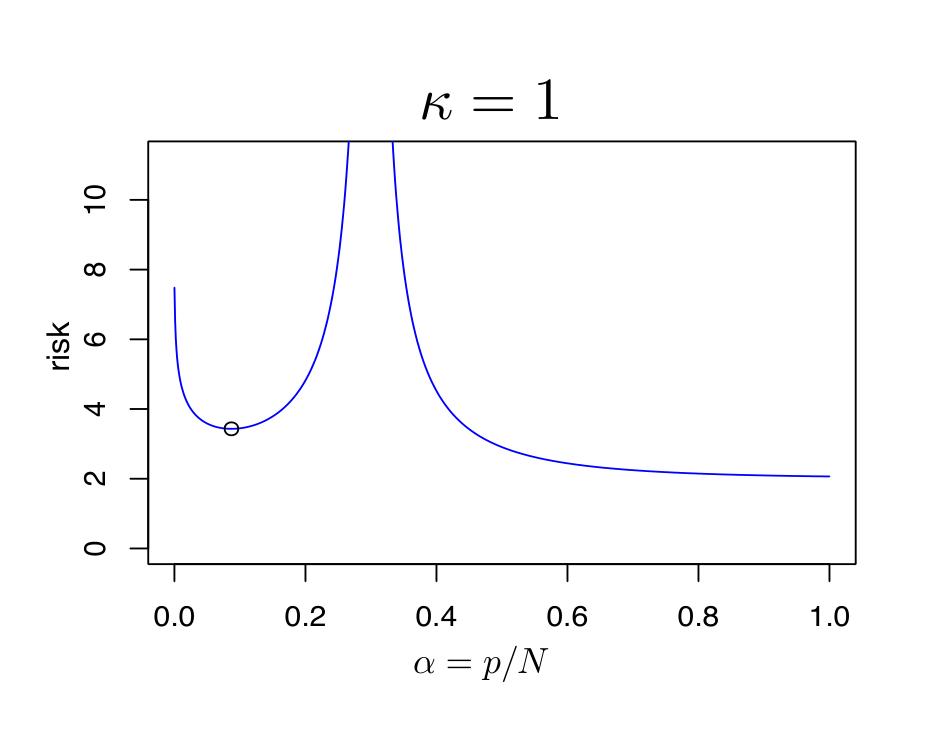
We plot the asymptotic risk function $\mathcal{R}_{\kappa}$ in Figure 1 for two different values of $\kappa$ , both with $\beta=0.3$ . (In simulations, we find that $\mathbb{E}_{\boldsymbol{\theta}}[\operatorname{Error}]$ matches these curves very closely for sample sizes as small as $n=300$ .) For both values of $\kappa\in\{1,2\}$ , we observe the striking “double descent” behavior as found in previous studies [2, e.g.,]. Moreover, we see that the asymptotic risk at $\alpha=1$ is smaller than the minimum asymptotic risk achieved at any $\alpha<\beta$ . This, in fact, happens for all values of $\kappa>0$ , as we claim in the next theorem.

Theorem 3.

Assume A.1 with constant $\kappa$ , A.2 with constants $\alpha$ and $\beta$ , $\sigma^{2}=0$ . Let $\alpha^{*}$ be the minimizer of $\mathcal{R}_{\kappa}$ over the interval $\mathinner{\left[0,\beta\right)}$ . Then $\limsup_{N}\mathcal{R}_{\kappa}(1)/\mathcal{R}_{\kappa}(\alpha^{*})<1$ . Moreover, $\mathcal{R}_{\kappa}(\alpha)/\mathcal{R}_{\kappa}(1)\to\infty$ as $\alpha\to\beta^{-}$ .

The proof of Theorem 3 is given in Section 2.4. Theorem 3 shows that the asymptotic risk exhibits a second decrease somewhere in the $p>n$ regime when $N$ is sufficiently large, and moreover, that it is possible to find a value of $p$ in this $p>n$ regime to achieve a lower asymptotic risk than any $p<n$ .

In the noisy setting (see Appendix C), it is possible for the asymptotic risk to be dominated by the noise, in which case the minimum asymptotic risk is in fact achieved by $\alpha=0$ (i.e., $p=o(n)$ ). However, there exists a regime with $\sigma^{2}>0$ in which we have the same conclusion as in Theorem 3.

Refer to caption — Figure 1: The asymptotic risk function $\mathcal{R}_{\kappa}$ as a function of $\alpha$ (with $n=300$ , $N=1000$ , $\beta=n/N=0.3$ and $\kappa=1,2$ respectively). The location of $\alpha^{*}$ from Theorem 1 is marked with a black circle. In both cases, the asymptotic risk at $\alpha=1$ is lower than the asymptotic risk at $\alpha^{*}$ .

2.2 Proof sketch for Theorem 1

We first show that $h_{\kappa}(\alpha)=0$ has a unique solution on $\mathinner{\left(0,\beta\right)}$ . Define $\tilde{h}_{\kappa}(\alpha)\mathrel{\mathop{\mathchar 58\relax}}=\alpha^{1-\kappa}h_{\kappa}(\alpha)$ . We shall show that $\tilde{h}_{\kappa}(\alpha)=0$ has a unique solution on $\mathinner{\left(0,\beta\right)}$ , which in turn immediately implies that $h_{\kappa}(\alpha)=0$ also has a unique solution on the same interval. Observe that

\frac{\dif\tilde{h}_{\kappa}(\alpha)}{\dif\alpha}=\frac{-\kappa\beta+\kappa\alpha}{\alpha^{1+\kappa}}<0.

(8)

Hence, the function $\tilde{h}_{\kappa}(\alpha)$ is strictly decreasing on $\alpha\in\mathinner{\left(0,\beta\right]}$ . Furthermore, we have

\tilde{h}_{\kappa}(\alpha)>0\ \ \text{as $\alpha\rightarrow 0^{+}$},\quad\text{and}\quad\tilde{h}_{\kappa}(\alpha)<0\ \ \text{at $\alpha=\beta$}.

(9)

Because $\tilde{h}_{\kappa}$ is continuous, it follows that the equation $\tilde{h}_{\kappa}(\alpha)=0$ has a unique solution on $\mathinner{\left(0,\beta\right)}$ .

We now prove $\mathbb{E}_{\boldsymbol{\theta}}[\operatorname{Error}]\stackrel{{\scriptstyle\mathrm{p}}}{{\rightarrow}}\mathcal{R}_{\kappa}(\alpha)$ . Since the proof only requires standard techniques, we just sketch the main ideas in this section, and leave the full proof to Appendix A. First, since $\alpha<\beta$ , for large enough $N$ , we have $p<n$ . Then the prediction error is given by

\displaystyle\operatorname{Error}

\displaystyle=

\displaystyle\mathbb{E}_{\boldsymbol{x},y}[(y-\boldsymbol{x}^{{\scriptscriptstyle{\top}}}\hat{\boldsymbol{\theta}})^{2}]\ =\ \|\boldsymbol{\Sigma}_{P}^{1/2}\left(\boldsymbol{X}_{P}^{{\scriptscriptstyle{\top}}}\boldsymbol{X}_{P}\right)^{-1}\boldsymbol{X}_{P}^{{\scriptscriptstyle{\top}}}\boldsymbol{X}_{P^{c}}\boldsymbol{\theta}_{P^{c}}\|^{2}+\|\boldsymbol{\Sigma}_{P^{c}}^{1/2}\boldsymbol{\theta}_{P^{c}}\|^{2},

where $\boldsymbol{\Sigma}_{P}\in\mathbb{R}^{p\times p}$ and $\boldsymbol{\Sigma}_{P^{c}}\in\mathbb{R}^{(N-p)\times(N-p)}$ are two diagonal matrices whose diagonal elements are the first $p$ and last $N-p$ diagonal elements of $\boldsymbol{\Sigma}$ , respectively. By (2), we have

\displaystyle\mathbb{E}_{\boldsymbol{\theta}}[\operatorname{Error}]

\displaystyle=

\displaystyle\operatorname{tr}(\boldsymbol{X}_{P^{c}}^{{\scriptscriptstyle{\top}}}\boldsymbol{X}_{P}\left(\boldsymbol{X}_{P}^{{\scriptscriptstyle{\top}}}\boldsymbol{X}_{P}\right)^{-1}\boldsymbol{\Sigma}_{P}\left(\boldsymbol{X}_{P}^{{\scriptscriptstyle{\top}}}\boldsymbol{X}_{P}\right)^{-1}\boldsymbol{X}_{P}^{{\scriptscriptstyle{\top}}}\boldsymbol{X}_{P^{c}})+\operatorname{tr}(\boldsymbol{\Sigma}_{P^{c}}).

Note that $\boldsymbol{X}_{P^{c}}$ is independent of $\boldsymbol{X}_{P}$ , thus, given $\boldsymbol{X}_{P}$ , the trace that includes $\boldsymbol{X}_{P^{c}}$ is a sum of $N-p$ independent random variables. Therefore, we have

$\displaystyle\mathbb{E}_{\boldsymbol{\theta}}[\operatorname{Error}]$	$\displaystyle\stackrel{{\scriptstyle\mathrm{p}}}{{\rightarrow}}$	$\displaystyle\operatorname{tr}(\boldsymbol{\Sigma}_{P^{c}})\cdot(\operatorname{tr}((\boldsymbol{X}_{P}^{{\scriptscriptstyle{\top}}}\boldsymbol{X}_{P})^{-1}\boldsymbol{\Sigma}_{P})+1)$
	$\displaystyle=$	$\displaystyle\operatorname{tr}(\boldsymbol{\Sigma}_{P^{c}})\cdot(\operatorname{tr}((\bar{\boldsymbol{X}}_{P}^{{\scriptscriptstyle{\top}}}\bar{\boldsymbol{X}}_{P})^{-1})+1)$
	$\displaystyle\stackrel{{\scriptstyle\mathrm{p}}}{{\rightarrow}}$	$\displaystyle\operatorname{tr}(\boldsymbol{\Sigma}_{P^{c}})\frac{\beta}{\beta-\alpha},$

where $\bar{\boldsymbol{X}}_{P}\mathrel{\mathop{\mathchar 58\relax}}=\boldsymbol{X}_{P}\boldsymbol{\Sigma}_{P}^{-1/2}$ is a standard Gaussian matrix. The first line above uses Markov’s inequality to show that $\mathbb{E}_{\boldsymbol{\theta}}[\operatorname{Error}]$ converges in probability to $\mathbb{E}_{\boldsymbol{\theta},\boldsymbol{X}_{P^{c}}}[\operatorname{Error}]$ . The third line above uses Assumption A.2 and the fact that $\bar{\boldsymbol{X}}_{P}^{{\scriptscriptstyle{\top}}}\bar{\boldsymbol{X}}_{P}$ is a standard Wishart matrix $\mathcal{W}_{p}(\boldsymbol{I},n)$ . So, to prove (4), we just need to compute $\operatorname{tr}(\boldsymbol{\Sigma}_{P^{c}})$ . Note that $\int_{s}^{s+1}t^{-\kappa}\dif t<s^{-\kappa}<\int_{s-1}^{s}t^{-\kappa}\dif t$ . Hence, we have

\displaystyle\int_{p+1}^{N}\frac{N^{\kappa}}{t^{\kappa}}\dif t\cdot\frac{1}{N}\ <\ \frac{N^{\kappa}}{N}\sum_{i=p+1}^{N}\frac{1}{i^{\kappa}}\ =N^{\kappa-1}\operatorname{tr}(\boldsymbol{\Sigma}_{P^{c}})\ <\ \int_{p}^{N}\frac{N^{\kappa}}{t^{\kappa}}\dif t\cdot\frac{1}{N}.

(10)

Therefore, we have $\operatorname{tr}(\boldsymbol{\Sigma}_{P^{c}})\rightarrow N^{1-\kappa}\int_{\alpha}^{1}t^{-\kappa}\dif t$ as $p\rightarrow\infty$ , and thus we have $\mathbb{E}_{\boldsymbol{\theta}}[\operatorname{Error}]\stackrel{{\scriptstyle\mathrm{p}}}{{\rightarrow}}\mathcal{R}_{\kappa}(\alpha)$ .

Finally, to prove (5), we analyze the shape of $\mathcal{R}_{\kappa}(\alpha)$ to find its minimum value over $\alpha<\beta$ . We take the derivative of $g_{\kappa}(\alpha)\mathrel{\mathop{\mathchar 58\relax}}=N^{\kappa-1}\mathcal{R}_{\kappa}(\alpha)$ :

\frac{\dif g_{\kappa}(\alpha)}{\dif\alpha}\ =\ \beta\cdot\frac{\alpha^{1-\kappa}-\beta\alpha^{-\kappa}+\int_{\alpha}^{1}t^{-\kappa}\dif t}{(\beta-\alpha)^{2}}\ =\ \frac{-\beta\alpha^{1-\kappa}\cdot h_{\kappa}(\alpha)}{(\beta-\alpha)^{2}}.

(11)

Using (8) and (9), we deduce that $\mathcal{R}_{\kappa}(\alpha)$ first decreases and then increases as a function of $\alpha$ in the interval $\mathinner{\left(0,\beta\right)}$ . Therefore, the minimum risk is achieved at the unique solution $\alpha^{*}$ of the equation $h_{\kappa}(\alpha)=0$ over the interval $\mathinner{\left(0,\beta\right)}$ . Equation (11) also implies $\int_{\alpha^{*}}^{1}t^{-\kappa}\dif t=(\beta-\alpha^{*})(\alpha^{*})^{-\kappa}$ . Hence, the minimum risk is given by

\min_{\alpha<\beta}\ \mathcal{R}_{\kappa}(\alpha)\ =\ N^{1-\kappa}\frac{\beta}{\beta-\alpha^{*}}\int_{\alpha^{*}}^{1}t^{-\kappa}\dif t\ =\ N^{1-\kappa}\frac{\beta}{(\alpha^{*})^{\kappa}}.

2.3 Proof sketch for Theorem 2

We first show that $m_{\kappa}(0)$ is well-defined. Consider the RHS expression from Equation 6 evaluated at $z=0$ ; by a change-of-variable in the integral, we have

\frac{1}{m}-\frac{1}{\beta}\int_{\alpha^{-\kappa}}^{\infty}\frac{\kappa^{-1}t^{-1/\kappa}}{1+t\cdot m}\dif t=\frac{1}{\beta\alpha m^{1-1/\kappa}}\left(\frac{\beta}{m^{1/\kappa}/\alpha}-\alpha\int_{m^{1/\kappa}/\alpha}^{\infty}\frac{t^{\kappa-2}}{1+t^{\kappa}}\dif t\right),

(12)

where $m=m_{\kappa}(0)$ . So, we just need to show that $q_{\kappa}(s,\alpha)=0$ has a unique solution $s^{*}_{\kappa}$ for $s$ over the positive real line, where $q_{\kappa}(s,\alpha)$ is defined by

\displaystyle q_{\kappa}(s,\alpha)\ \mathrel{\mathop{\mathchar 58\relax}}=\ \frac{\beta}{s}-\alpha\int_{s}^{\infty}\frac{t^{\kappa-2}}{1+t^{\kappa}}\dif t.

(13)

(This makes $m_{\kappa}(0)$ well-defined, via the equation $s^{*}_{\kappa}=m_{\kappa}(0)^{1/\kappa}/\alpha$ , and also verifies its positivity.)

The derivative of $q_{\kappa}(s,\alpha)$ with respect to $s$ is

\displaystyle\frac{\partial q_{\kappa}(s,\alpha)}{\partial s}

\displaystyle=

\displaystyle\frac{(\alpha-\beta)s^{\kappa}-\beta}{s^{2}(1+s^{\kappa})}.

(14)

Hence, since $\alpha>\beta$ , we know the function $q_{\kappa}(s,\alpha)$ is strictly decreasing on $s\in(0,(\frac{\beta}{\alpha-\beta})^{1/\kappa}]$ and strictly increasing on $s\in[(\frac{\beta}{\alpha-\beta})^{1/\kappa},\infty)$ . Furthermore, $q_{\kappa}(s,\alpha)\rightarrow\infty$ as $s\rightarrow 0$ and $q_{\kappa}(s,\alpha)\rightarrow 0$ as $s\rightarrow\infty$ . Hence, by the continuity of $s\mapsto q_{\kappa}(s,\alpha)$ , we conclude that $q_{\kappa}(s,\alpha)=0$ has a unique solution $s^{*}_{\kappa}$ .

Using the chain rule, we can also show that $m_{\kappa}^{\prime}(0)$ is well-defined, and that its value is given by

m_{\kappa}^{\prime}(0)\ =\ \kappa\beta m^{2}_{\kappa}(0)\cdot(1+(s^{*}_{\kappa})^{\kappa})/\left(\beta+(\beta-\alpha)(s^{*}_{\kappa})^{\kappa}\right)>0.

We leave the details to Section B.1.

Our next goal is to prove $\mathbb{E}_{\boldsymbol{\theta}}[\operatorname{Error}]\stackrel{{\scriptstyle\mathrm{p}}}{{\rightarrow}}\mathcal{R}_{\kappa}(\alpha)$ . Since $\alpha>\beta$ , we have $p>n$ for large enough $N$ . In this case,

	$\displaystyle\operatorname{Error}$	$\displaystyle=$	$\displaystyle\mathbb{E}_{\boldsymbol{x},y}[(y-\boldsymbol{x}^{{\scriptscriptstyle{\top}}}\hat{\boldsymbol{\theta}})^{2}]\ =\ \mathbb{E}_{\boldsymbol{x},y}[(\boldsymbol{x}_{P}^{{\scriptscriptstyle{\top}}}(\hat{\boldsymbol{\theta}}_{P}-\boldsymbol{\theta}_{P})-\boldsymbol{x}_{P^{c}}^{{\scriptscriptstyle{\top}}}\boldsymbol{\theta}_{P^{c}})^{2}]$
		$\displaystyle=$	$\displaystyle\\|\boldsymbol{\Sigma}_{P}^{1/2}((\boldsymbol{\Pi}_{\boldsymbol{X}_{P}}-\boldsymbol{I})\boldsymbol{\theta}_{P}+\boldsymbol{X}_{P}^{{\scriptscriptstyle{\top}}}(\boldsymbol{X}_{P}\boldsymbol{X}_{P}^{{\scriptscriptstyle{\top}}})^{-1}\boldsymbol{X}_{P^{c}}\boldsymbol{\theta}_{P^{c}})\\|^{2}+\\|\boldsymbol{\Sigma}_{P^{c}}^{1/2}\boldsymbol{\theta}_{P^{c}}\\|^{2},$

where $\boldsymbol{\Pi}_{\boldsymbol{X}_{P}}\mathrel{\mathop{\mathchar 58\relax}}=\boldsymbol{X}_{P}^{{\scriptscriptstyle{\top}}}\left(\boldsymbol{X}_{P}\boldsymbol{X}_{P}^{{\scriptscriptstyle{\top}}}\right)^{-1}\boldsymbol{X}_{P}$ , and the diagonal matrices $\boldsymbol{\Sigma}_{P}$ and $\boldsymbol{\Sigma}_{P^{c}}$ are as defined in Section 2.2. Hence, $\mathbb{E}_{\boldsymbol{\theta}}[\operatorname{Error}]$ is equal to

\underbrace{\operatorname{tr}(\boldsymbol{\Sigma}_{P}(\boldsymbol{I}-\boldsymbol{\Pi}_{\boldsymbol{X}_{P}}))}_{\text{part 1}}+\underbrace{\operatorname{tr}(\boldsymbol{X}_{P^{c}}^{{\scriptscriptstyle{\top}}}(\boldsymbol{X}_{P}\boldsymbol{X}_{P}^{{\scriptscriptstyle{\top}}})^{-1}\boldsymbol{X}_{P}\boldsymbol{\Sigma}_{P}\boldsymbol{X}_{P}^{{\scriptscriptstyle{\top}}}(\boldsymbol{X}_{P}\boldsymbol{X}_{P}^{{\scriptscriptstyle{\top}}})^{-1}\boldsymbol{X}_{P^{c}})+\operatorname{tr}(\boldsymbol{\Sigma}_{P^{c}})}_{\text{part 2}}.

(15)

We claim that

part 1

\displaystyle\stackrel{{\scriptstyle\mathrm{p}}}{{\rightarrow}}

\displaystyle\frac{N^{1-\kappa}\beta}{m_{\kappa}(0)},\quad\text{and}\quad\text{part 2}\ \stackrel{{\scriptstyle\mathrm{p}}}{{\rightarrow}}\ N^{1-\kappa}\cdot\frac{m_{\kappa}^{\prime}(0)}{m^{2}_{\kappa}(0)}\cdot\int_{\alpha}^{1}t^{\kappa-2}\dif t+o_{\mathrm{p}}(N^{1-\kappa});

(16)

together, they complete the proof that $\mathbb{E}_{\boldsymbol{\theta}}[\operatorname{Error}]\stackrel{{\scriptstyle\mathrm{p}}}{{\rightarrow}}\mathcal{R}_{\kappa}(\alpha)$ . Rigorous proofs of the claims in (16) are presented in Section B.2 and Section B.3; here, we give a heuristic argument that conveys the main idea. For part 1, let $\tilde{\boldsymbol{\Sigma}}_{P}=N^{\kappa}\boldsymbol{\Sigma}_{P}$ and $\tilde{\boldsymbol{X}}_{P}=N^{\kappa/2}\boldsymbol{X}_{P}$ . This scaling ensures that the empirical eigenvalue distribution of $\tilde{\boldsymbol{\Sigma}}_{P}$ has a limiting distribution with probability density

f_{\kappa}(s)=\frac{1}{\kappa\alpha}s^{-1-1/\kappa}\cdot\mathds{1}_{\{s\in[\alpha^{-\kappa},\infty)\}}

(Lemma 2 in Section B.2). Also, under this scaling, we have

	$\displaystyle\operatorname{tr}(\boldsymbol{\Sigma}_{P}\left(\boldsymbol{I}-\boldsymbol{\Pi}_{\boldsymbol{X}_{P}}\right))\ =\ \lim_{\mu\rightarrow 0}\frac{n}{N^{\kappa}}\left(\frac{1}{n}\operatorname{tr}(\tilde{\boldsymbol{\Sigma}}_{P})-\frac{1}{n}\operatorname{tr}(\tilde{\boldsymbol{\Sigma}}_{P}(\tilde{\boldsymbol{X}}_{P}^{{\scriptscriptstyle{\top}}}\tilde{\boldsymbol{X}}_{P}+\mu n\boldsymbol{I})^{-1}\tilde{\boldsymbol{X}}_{P}^{{\scriptscriptstyle{\top}}}\tilde{\boldsymbol{X}}_{P})\right)$				(17)
		$\displaystyle=$	$\displaystyle\lim_{\mu\rightarrow 0}\frac{n}{N^{\kappa}}\cdot\frac{\mu}{n}\operatorname{tr}\left(\tilde{\boldsymbol{\Sigma}}_{P}\left(\frac{1}{n}\tilde{\boldsymbol{X}}_{P}^{{\scriptscriptstyle{\top}}}\tilde{\boldsymbol{X}}_{P}+\mu\boldsymbol{I}\right)^{-1}\right)\ =\ \lim_{\mu\rightarrow 0}\frac{n}{N^{\kappa}}\cdot\frac{\mu}{n}\operatorname{tr}(\tilde{\boldsymbol{\Sigma}}_{P}\tilde{\boldsymbol{S}}_{n}),$		(17)

where $\tilde{\boldsymbol{S}}_{n}\mathrel{\mathop{\mathchar 58\relax}}=(n^{-1}\tilde{\boldsymbol{X}}_{P}^{{\scriptscriptstyle{\top}}}\tilde{\boldsymbol{X}}_{P}+\mu\boldsymbol{I})^{-1}$ . As long as the empirical eigenvalue distribution of $\tilde{\boldsymbol{\Sigma}}_{P}$ has a limiting distribution with bounded support, we have

\displaystyle\forall\mu>0,\quad\mu\cdot\frac{1}{n}\operatorname{tr}\left(\tilde{\boldsymbol{\Sigma}}_{P}\left(\frac{1}{n}\tilde{\boldsymbol{X}}_{P}^{{\scriptscriptstyle{\top}}}\tilde{\boldsymbol{X}}_{P}+\mu\boldsymbol{I}\right)^{-1}\right)\ \stackrel{{\scriptstyle\mathrm{p}}}{{\rightarrow}}\ \frac{1}{m_{\kappa}(-\mu)},

(18)

where $m_{\kappa}(z)$ is, in fact, the Stieltjes transform of the limiting empirical eigenvalue distribution of $n^{-1}\tilde{\boldsymbol{X}}_{P}\tilde{\boldsymbol{X}}_{P}^{{\scriptscriptstyle{\top}}}$ (Lemma 1 in Section B.2); this follows from results of Dobriban and Wager 2018, which in turn are derived from the results of Ledoit and Péché 2011. Assume we can exchange the two limits $\mu\rightarrow 0^{+}$ and $N\rightarrow\infty$ , and also that (18) still holds for $f_{\kappa}(s)$ which has unbounded support. Then, from (17), we conclude

\displaystyle\text{part 1}\ =\ \operatorname{tr}(\boldsymbol{\Sigma}_{P}\left(\boldsymbol{I}-\boldsymbol{\Pi}_{\boldsymbol{X}_{P}}\right))\ \stackrel{{\scriptstyle\mathrm{p}}}{{\rightarrow}}\ \frac{N^{1-\kappa}\beta}{m_{\kappa}(0)}.

For part 2, note that $\boldsymbol{X}_{P^{c}}$ is independent of $\boldsymbol{X}_{P}$ . Thus, conditional on $\boldsymbol{X}_{P}$ , part 2 is a sum of $N-p$ independent random variables. Therefore, using Markov inequality, we can show that

part 2	$\displaystyle\stackrel{{\scriptstyle\mathrm{p}}}{{\rightarrow}}$	$\displaystyle\mathbb{E}_{\boldsymbol{X}_{P^{c}}}[\text{part 2}]\ =\ \operatorname{tr}\left(\boldsymbol{\Sigma}_{P^{c}}\right)\cdot\left(\operatorname{tr}\left(\boldsymbol{\Sigma}_{P}\boldsymbol{X}_{P}^{{\scriptscriptstyle{\top}}}\left(\boldsymbol{X}_{P}\boldsymbol{X}_{P}^{{\scriptscriptstyle{\top}}}\right)^{-2}\boldsymbol{X}_{P}\right)+1\right)$	(19)
	$\displaystyle=$	$\displaystyle\operatorname{tr}\left(\boldsymbol{\Sigma}_{P^{c}}\right)\cdot\left(\lim_{\mu\rightarrow 0}\operatorname{tr}\left(\tilde{\boldsymbol{\Sigma}}_{P}\left(\tilde{\boldsymbol{X}}_{P}^{{\scriptscriptstyle{\top}}}\tilde{\boldsymbol{X}}_{P}+\mu n\boldsymbol{I}\right)^{-1}\tilde{\boldsymbol{X}}_{P}^{{\scriptscriptstyle{\top}}}\tilde{\boldsymbol{X}}_{P}\left(\tilde{\boldsymbol{X}}_{P}^{{\scriptscriptstyle{\top}}}\tilde{\boldsymbol{X}}_{P}+\mu n\boldsymbol{I}\right)^{-1}\right)+1\right)$
	$\displaystyle=$	$\displaystyle\operatorname{tr}\left(\boldsymbol{\Sigma}_{P^{c}}\right)\cdot\left(\lim_{\mu\rightarrow 0}\frac{1}{n}\operatorname{tr}\left(\tilde{\boldsymbol{\Sigma}}_{P}\tilde{\boldsymbol{S}}_{n}\right)-\frac{\mu}{n}\operatorname{tr}\left(\tilde{\boldsymbol{\Sigma}}_{P}\tilde{\boldsymbol{S}}_{n}^{2}\right)+1\right).$

Again, if we ignore the fact that the support of $f_{\kappa}(s)$ is unbounded and assume the limits of $\mu\rightarrow 0$ and $N\rightarrow\infty$ can be exchanged, then by Lemma 7.4 of Dobriban and Wager 2018, we have

\displaystyle\text{part 2}\ \stackrel{{\scriptstyle\mathrm{p}}}{{\rightarrow}}\ \operatorname{tr}\left(\boldsymbol{\Sigma}_{P^{c}}\right)\cdot\left(\lim_{\mu\rightarrow 0}\frac{1}{n}\operatorname{tr}\left(\tilde{\boldsymbol{\Sigma}}_{P}\tilde{\boldsymbol{S}}_{n}\right)-\frac{\mu}{n}\operatorname{tr}\left(\tilde{\boldsymbol{\Sigma}}_{P}\tilde{\boldsymbol{S}}_{n}^{2}\right)+1\right)\stackrel{{\scriptstyle\mathrm{p}}}{{\rightarrow}}\operatorname{tr}\left(\boldsymbol{\Sigma}_{P^{c}}\right)\cdot\frac{m_{\kappa}^{\prime}(0)}{m_{\kappa}^{2}(0)}.

(20)

A straightforward analysis of $\operatorname{tr}(\boldsymbol{\Sigma}_{P^{c}})$ (as in (10)) completes the analysis of part 2 of (16).

Remark 1.

Although Theorem 2 should intuitively hold given the results of Dobriban and Wager 2018, a careful and more involved argument is needed to deal with the facts that $\|\tilde{\boldsymbol{\Sigma}}_{P}\|_{2}\rightarrow\infty$ (since $\|\boldsymbol{\Sigma}_{P}^{-1}\|_{2}\rightarrow\infty$ ) and $\mu\rightarrow 0$ . For example, standard techniques only imply $\frac{\mu}{n}\operatorname{tr}(\tilde{\boldsymbol{\Sigma}}_{P}\tilde{\boldsymbol{S}}_{n})=O_{\mathrm{p}}(N^{\kappa})$ . However, we need the stronger bound $\frac{\mu}{n}\operatorname{tr}(\tilde{\boldsymbol{\Sigma}}_{P}\tilde{\boldsymbol{S}}_{n})=O_{\mathrm{p}}(1)$ (e.g., Section B.2.2).

2.4 Proof of Theorem 3

Comparing the expression for $\mathcal{R}_{\kappa}(\alpha)$ in (7) at $\alpha=1$ to the expression for $\mathcal{R}_{\kappa}(\alpha^{*})$ in (5), we see that it suffices to prove $m_{\kappa}(0)^{1/\kappa}>\alpha^{*}$ . Recall that in Section 2.3, we have proved $s^{*}_{\kappa}\mathrel{\mathop{\mathchar 58\relax}}=m_{\kappa}(0)^{1/\kappa}$ is the unique solution of the equation $q_{\kappa}(s,1)=0$ . Furthermore, using the expression for the derivative of $q_{\kappa}(s,1)$ with respect to $s$ in (14), we know that $q(s,1)>0\Rightarrow s<s^{*}_{\kappa}$ . Thus, we only need to show $q_{\kappa}(\alpha^{*},1)>0=h_{\kappa}(\alpha^{*})$ , where the equality is due to the definition of $\alpha^{*}$ in Theorem 1. Note that by the definitions of the functions $q_{\kappa}$ and $h_{\kappa}$ in (3) and (13), we have

\displaystyle h_{\kappa}(s)

\displaystyle=

\displaystyle\frac{\beta}{s}-\int_{s}^{1}t^{\kappa-2}\dif t-1\ =\ q_{\kappa}(s,1)+\int_{s}^{\infty}\frac{t^{\kappa-2}}{(1+t^{\kappa})}\dif t-\int_{s}^{1}t^{\kappa-2}\dif t-1.

Furthermore, $h_{\kappa}(s)-q_{\kappa}(s,1)$ is increasing in $s$ :

\displaystyle\frac{\dif~(h_{\kappa}(s)-q_{\kappa}(s,1))}{\dif s}

\displaystyle=

\displaystyle-\frac{s^{\kappa-2}}{(1+s^{\kappa})}+s^{\kappa-2}\ =\ \frac{s^{2\kappa-2}}{1+s^{\kappa}}\ >\ 0.

Hence, for all for all $s\in\mathinner{\left(0,1\right]}$ , we have

	$\displaystyle h_{\kappa}(s)-q_{\kappa}(s,1)$	$\displaystyle\leq$	$\displaystyle h_{\kappa}(1)-q_{\kappa}(1,1)\ =\ \int_{1}^{\infty}\frac{t^{\kappa-2}}{(1+t^{\kappa})}\dif t-1$
		$\displaystyle=$	$\displaystyle\int_{1}^{\infty}\frac{t^{\kappa-2}}{(1+t^{\kappa})}\dif t-\int_{1}^{\infty}\frac{1}{t^{2}}\dif t\ =\ -\int_{1}^{\infty}\frac{1}{t^{2}(1+t^{\kappa})}\dif t\ <\ 0.$

Since $\alpha^{*}<\beta<1$ , we have $0=h_{\kappa}(\alpha^{*})<q_{\kappa}(\alpha^{*},1)$ , and thus we have $s^{*}_{\kappa}>\alpha^{*}$ .

By inspection of the expression for $\mathcal{R}_{\kappa}(\alpha)$ in (4), it is also clear that $\mathcal{R}_{\kappa}(\alpha)/\mathcal{R}_{\kappa}(1)\rightarrow\infty$ as $\alpha\rightarrow\beta^{-}$ .

3 Analysis under general eigenvalue decay

In this section, we extend the results from Section 2 (with noise) to hold under a more general assumption on the eigenvalues of $\boldsymbol{\Sigma}$ . To simplify calculations, we use a slightly different feature selection procedure that includes all components $j$ such that $\lambda_{j}\geq\nu_{N}$ , so $p=\sum_{j=1}^{N}\mathds{1}_{\{\lambda_{j}\geq\nu_{N}\}}$ .

Instead of Assumptions A.1 and A.2, we assume the following:

B.1

$\|\boldsymbol{\Sigma}\|_{2}\leq C$ for some constant $C>0$ . Also, there exists a positive sequence $(c_{N})_{N\geq 1}$ such that the empirical eigenvalue distribution of $c_{N}\boldsymbol{\Sigma}$ converges as $N\to\infty$ to $F=(1-\delta)F_{0}+\delta F_{1}$ , where $\delta\in(0,1]$ , $F_{0}$ is a point mass of $0$ , and $F_{1}$ has a continuous probability density $f$ supported on either $\mathinner{\left[\eta_{1},\eta_{2}\right]}$ or $\mathinner{\left[\eta_{1},\infty\right)}$ for some constants $\eta_{1},\eta_{2}>0$ .
B.2

There exist constants $\nu>0$ and $\beta\in\mathinner{\left(0,\delta\right)}$ s.t. $\nu_{N}c_{N}\to\nu$ and $n/N\to\beta$ as $n,N\to\infty$ .

The $c_{N}$ in Assumption B.1 generalizes the $N^{\kappa}$ scaling introduced in the proof of Theorem 2. In fact, Assumption B.1 is more general than the eigenvalue assumptions made by Dobriban and Wager 2018 and Hastie et al. 2019: the eigenvalues of $\boldsymbol{\Sigma}$ could decrease smoothly ( $\delta=1$ ), or there could be a sudden drop between (say) $\lambda_{j}$ and $\lambda_{j+1}$ ( $\delta<1$ ). Since $p$ is now determined by $\nu$ , whether $p<n$ or $p>n$ is now determined by whether $\nu>\nu_{b}$ or $\nu<\nu_{b}$ , where $\nu_{b}>\eta_{1}$ is given by the equation $\delta\int_{\nu_{b}}^{\infty}f(t)\dif t=\beta$ . Finally, by Assumption B.1,

\displaystyle\frac{p}{N}\ =\ \frac{1}{N}\sum_{j=1}^{N}\mathds{1}_{\{c_{N}\lambda_{j}\geq\nu\}}\ \stackrel{{\scriptstyle\mathrm{a.s.}}}{{\rightarrow}}\ \delta\mathbb{E}_{s\sim f}[\mathds{1}_{\{s\geq\nu\}}]\ =\ \delta\int_{\nu}^{\infty}f(t)\dif t\ =\mathrel{\mathop{\mathchar 58\relax}}\ \alpha(\nu),\quad\forall\nu>0.

(21)

For $\nu=0$ , i.e., $\nu_{N}=o(1/c_{N})$ , we choose $\nu_{N}$ be the $\delta N$ largest eigenvalues of $\boldsymbol{\Sigma}$ , then $\alpha(\nu)=\delta$ . Hence, combined with Assumption B.2, we have the same asymptotics considered in Section 2, except that $\beta$ is now restricted in $(0,\delta)$ . This restriction on $\beta$ is required, otherwise both $c_{N}\boldsymbol{X}^{{\scriptscriptstyle{\top}}}\boldsymbol{X}$ and $c_{N}\boldsymbol{X}\boldsymbol{X}^{{\scriptscriptstyle{\top}}}$ are asymptotically singular.

The following theorem generalizes the results in Section 2 to hold under Assumptions B.1 and B.2.

Theorem 4.

Assume B.1 with sequence $(c_{N})_{N\geq 1}$ and constants $C$ , $\delta$ , $\eta_{1}$ , and $\eta_{2}$ ; and B.2 with constants $\nu$ and $\beta$ .

(i)

Assume $\nu\in(\nu_{b},\infty)$ . Then

\displaystyle\mathbb{E}_{\boldsymbol{w},\boldsymbol{\theta}}[\operatorname{Error}]\ \stackrel{{\scriptstyle\mathrm{p}}}{{\rightarrow}}\ \left(\frac{N}{c_{N}}\cdot\delta\int_{\eta_{1}}^{\nu}tf(t)\dif t+\sigma^{2}\right)\frac{\beta}{\beta-\delta\int_{\nu}^{\infty}f(t)\dif t}\ =\mathrel{\mathop{\mathchar 58\relax}}\ \mathcal{R}_{f}(\nu,\sigma).

(22)

Define $h_{f}(\nu)\mathrel{\mathop{\mathchar 58\relax}}=\nu\beta-\nu\delta\int_{\nu}^{\infty}f(t)\dif t-\delta\int_{\eta_{1}}^{\nu}tf(t)\dif t$ . If the equation $h_{f}(\nu)=0$ has a solution on $(\nu_{b},\infty)\bigcap\text{supp}(f)$ , then the solution $\nu^{*}$ is unique, and

\mathcal{R}_{f}(\nu^{*},0)\ =\ \min_{\nu\in(\nu_{b},\infty)}\mathcal{R}_{f}(\nu,0)\ =\ \frac{N\beta}{c_{N}}\cdot\nu^{*}.

(23)

Otherwise,

\inf_{\nu\in(\nu_{b},\infty)}\mathcal{R}_{f}(\nu,0)\ =\ \lim_{\nu\to\infty}\mathcal{R}_{f}(\nu,0)\ =\ \frac{N}{c_{N}}\delta\int_{\eta_{1}}^{\infty}tf(t)\dif t.

(24)

(ii)

Assume $\nu\in\mathinner{\left[0,\nu_{b}\right)}$ . Define $q_{f}(s,\nu)\mathrel{\mathop{\mathchar 58\relax}}=s\beta-s\delta\int_{\nu}^{\infty}\frac{tf(t)}{s+t}\dif t$ . Then

\displaystyle\mathbb{E}_{\boldsymbol{w},\boldsymbol{\theta}}[\operatorname{Error}]

\displaystyle\stackrel{{\scriptstyle\mathrm{p}}}{{\rightarrow}}

\displaystyle\frac{N\beta}{c_{N}}s^{*}_{f}+\beta\cdot\frac{\frac{N}{c_{N}}\delta\int_{\eta_{1}}^{\nu}tf(t)\dif t+\sigma^{2}}{\delta s^{*}_{f}\int_{\nu}^{\infty}\frac{tf(t)}{(s^{*}_{f}+t)^{2}}\dif t}\ =\mathrel{\mathop{\mathchar 58\relax}}\ \mathcal{R}_{f}(\nu,\sigma),

(25)

where $s^{*}_{f}$ is the unique solution of the equation $q_{f}(s,\nu)=0$ .

(iii)

Suppose $\sigma=0$ . Let $\nu^{*}$ be the minimizer of $\mathcal{R}_{f}(\nu,0)$ over the interval $(\nu_{b},\infty]$ (including $\infty$ ). Let $\mathcal{R}_{f}(\eta_{1},0)$ be the risk achieved at $\nu=\eta_{1}$ . Then $\limsup_{N}\mathcal{R}_{f}(\eta_{1},0)/\mathcal{R}_{f}(\nu^{*},0)<1$ .

The proof of this theorem is presented in Appendix D.

4 Discussion

Our results confirm the emergence of the “double descent” risk curve in a natural setting with Gaussian design. As in previous works [3, 8, 13, e.g.,], the shape emerges when there is a spike at the interpolation threshold ( $p=n$ ), which is typically caused by a near-zero minimum eigenvalue of the empirical covariance matrix.

More importantly, however, our results shed light on when the minimum risk is achieved before or after the interpolation threshold in terms of the noise level and eigenvalues of the (population) covariance matrix. For instance, when the eigenvalues decay very slowly or not at all ( $\kappa<1$ ), a smaller risk is achieved after the interpolation threshold ( $p>n$ ) than any point before ( $p<n$ ). On the other hand, when the eigenvalues decay more quickly ( $\kappa>1$ ), a smaller risk is achieved in the $p>n$ regime only in the noiseless setting. In general, the $p<n$ regime yields a smaller risk when the noise dominates the error due to model misspecification. Providing a full characterization is an important direction for future research.

Finally, we point out that the PCR estimator we study is a non-standard “oracle” estimator because it generally requires knowledge of $\boldsymbol{\Sigma}$ . Although it can be plausibly implemented in a semi-supervised setting (by estimating $\boldsymbol{\Sigma}$ very accurately using unlabeled data), a full analysis that accounts for estimation errors in $\boldsymbol{\Sigma}$ , or of a more standard PCR estimator, remains open. However, we note that the PCR estimator with $p=N$ can be implemented, and in our analysis, the dominance of the $p>n$ regime is always established at $p=N$ . We believe that this should be true for the standard PCR estimator as well.

Acknowledgments

This research was supported by NSF CCF-1740833, a Sloan Research Fellowship, a Google Faculty Award, and a Cheung-Kong Graduate School of Business Fellowship.

References

Bauer et al. [2007] Frank Bauer, Sergei Pereverzev, and Lorenzo Rosasco. On regularization algorithms in learning theory. Journal of complexity, 23(1):52–72, 2007.
Belkin et al. [2018] Mikhail Belkin, Daniel Hsu, Siyuan Ma, and Soumik Mandal. Reconciling modern machine learning and the bias-variance trade-off. arXiv preprint arXiv:1812.11118, 2018.
Belkin et al. [2019] Mikhail Belkin, Daniel Hsu, and Ji Xu. Two models of double descent for weak features. arXiv preprint arXiv:1903.07571, 2019.
Breiman and Freedman [1983] Leo Breiman and David Freedman. How many variables should be entered in a regression equation? Journal of the American Statistical Association, 78(381):131–136, 1983.
Dicker [2016] Lee H Dicker. Ridge regression and asymptotic minimax estimation over spheres of growing dimension. Bernoulli, 22(1):1–37, 2016.
Dobriban and Wager [2018] Edgar Dobriban and Stefan Wager. High-dimensional asymptotics of prediction: Ridge regression and classification. The Annals of Statistics, 46(1):247–279, 2018.
Gerfo et al. [2008] L Lo Gerfo, Lorenzo Rosasco, Francesca Odone, Ernesto De Vito, and Alessandro Verri. Spectral algorithms for supervised learning. Neural Computation, 20(7):1873–1897, 2008.
Hastie et al. [2019] Trevor Hastie, Andrea Montanari, Saharon Rosset, and Ryan J Tibshirani. Surprises in high-dimensional ridgeless least squares interpolation. arXiv preprint arXiv:1903.08560, 2019.
Jolliffe [2011] Ian Jolliffe. Principal Component Analysis. Springer, 2011.
Laurent and Massart [2000] Beatrice Laurent and Pascal Massart. Adaptive estimation of a quadratic functional by model selection. Annals of Statistics, pages 1302–1338, 2000.
Ledoit and Péché [2011] Olivier Ledoit and Sandrine Péché. Eigenvectors of some large sample covariance matrix ensembles. Probability Theory and Related Fields, 151(1-2):233–264, 2011.
Mathé [2004] Peter Mathé. Saturation of regularization methods for linear ill-posed problems in hilbert spaces. SIAM journal on numerical analysis, 42(3):968–973, 2004.
Muthukumar et al. [2019] Vidya Muthukumar, Kailas Vodrahalli, and Anant Sahai. Harmless interpolation of noisy data in regression. arXiv preprint arXiv:1903.09139, 2019.
Neal et al. [2018] Brady Neal, Sarthak Mittal, Aristide Baratin, Vinayak Tantia, Matthew Scicluna, Simon Lacoste-Julien, and Ioannis Mitliagkas. A modern take on the bias-variance tradeoff in neural networks. arXiv preprint arXiv:1810.08591, 2018.
Rahimi and Recht [2008] Ali Rahimi and Benjamin Recht. Random features for large-scale kernel machines. In Advances in Neural Information Processing Systems, pages 1177–1184, 2008.
Silverstein and Choi [1995] Jack W Silverstein and Sang-Il Choi. Analysis of the limiting spectral distribution of large dimensional random matrices. Journal of Multivariate Analysis, 54(2):295–309, 1995.
Spigler et al. [2018] Stefano Spigler, Mario Geiger, Stéphane d’Ascoli, Levent Sagun, Giulio Biroli, and Matthieu Wyart. A jamming transition from under-to over-parametrization affects loss landscape and generalization. arXiv preprint arXiv:1810.09665, 2018.
Tulino and Verdú [2004] Antonia M Tulino and Sergio Verdú. Random matrix theory and wireless communications. Foundations and Trends in Communications and Information Theory, 1(1):1–182, 2004.
Xu et al. [2019] Ji Xu, Arian Maleki, and Kamiar Rahnama Rad. Consistent risk estimation in high-dimensional linear regression. arXiv preprint arXiv:1902.01753, 2019.

Appendix A Proof of Theorem 1

The full proof for Theorem 1 is presented in this section. Since $\alpha<\beta$ , we have $p<n$ hold for large enough $N$ . Then, the least square estimate $\hat{\boldsymbol{\theta}}_{P}$ is given by $\left(\boldsymbol{X}_{P}^{{\scriptscriptstyle{\top}}}\boldsymbol{X}_{P}\right)^{-1}\boldsymbol{X}_{P}^{{\scriptscriptstyle{\top}}}\boldsymbol{X}\boldsymbol{\theta}$ and the prediction error is given by

	$\displaystyle\operatorname{Error}$	$\displaystyle=$	$\displaystyle\mathbb{E}_{\boldsymbol{x},y}[(y-\boldsymbol{x}^{{\scriptscriptstyle{\top}}}\hat{\boldsymbol{\theta}})^{2}]\ =\ \mathbb{E}_{\boldsymbol{x},y}[(\boldsymbol{x}_{P}^{{\scriptscriptstyle{\top}}}(\boldsymbol{\theta}_{P}-\hat{\boldsymbol{\theta}}_{P})+\boldsymbol{x}_{P^{c}}^{{\scriptscriptstyle{\top}}}\boldsymbol{\theta}_{P^{c}})^{2}]$
		$\displaystyle=$	$\displaystyle\\|\boldsymbol{\Sigma}_{P}^{1/2}(\boldsymbol{X}_{P}^{{\scriptscriptstyle{\top}}}\boldsymbol{X}_{P})^{-1}\boldsymbol{X}_{P}^{{\scriptscriptstyle{\top}}}\boldsymbol{X}_{P^{c}}\boldsymbol{\theta}_{P^{c}}\\|^{2}+\\|\boldsymbol{\Sigma}_{P^{c}}^{1/2}\boldsymbol{\theta}_{P^{c}}\\|^{2},$

where $\boldsymbol{\Sigma}_{P}\in\mathbb{R}^{p\times p}$ and $\boldsymbol{\Sigma}_{P^{c}}\in\mathbb{R}^{(N-p)\times(N-p)}$ are the two diagonal matrices whose diagonal elements are the first $p$ and last $N-p$ diagonal elements of $\boldsymbol{\Sigma}$ respectively. By our assumption on $\boldsymbol{\theta}$ , we have

\displaystyle\mathbb{E}_{\boldsymbol{\theta}}[\operatorname{Error}]

\displaystyle=

\displaystyle\operatorname{tr}(\boldsymbol{X}_{P^{c}}^{{\scriptscriptstyle{\top}}}\boldsymbol{X}_{P}(\boldsymbol{X}_{P}^{{\scriptscriptstyle{\top}}}\boldsymbol{X}_{P})^{-1}\boldsymbol{\Sigma}_{P}(\boldsymbol{X}_{P}^{{\scriptscriptstyle{\top}}}\boldsymbol{X}_{P})^{-1}\boldsymbol{X}_{P}^{{\scriptscriptstyle{\top}}}\boldsymbol{X}_{P^{c}})+\operatorname{tr}(\boldsymbol{\Sigma}_{P^{c}}).

Our next step is to apply Markov inequality to show (4). Note that $\boldsymbol{X}_{P^{c}}$ is independent of $\boldsymbol{X}_{P}$ . Hence, the expectation of $\operatorname{Error}$ given $\boldsymbol{X}_{P}$ is the following:

	$\displaystyle\mathbb{E}[\operatorname{Error}\mid\boldsymbol{X}_{P}]$	$\displaystyle=$	$\displaystyle\operatorname{tr}(\boldsymbol{\Sigma}_{P^{c}})\cdot(\operatorname{tr}((\boldsymbol{X}_{P}^{{\scriptscriptstyle{\top}}}\boldsymbol{X}_{P})^{-1}\boldsymbol{\Sigma}_{P})+1)$		(26)
		$\displaystyle=$	$\displaystyle\operatorname{tr}(\boldsymbol{\Sigma}_{P^{c}})\cdot(\operatorname{tr}((\bar{\boldsymbol{X}}_{P}^{{\scriptscriptstyle{\top}}}\bar{\boldsymbol{X}}_{P})^{-1})+1),$		(26)

where $\bar{\boldsymbol{X}}_{P}=\boldsymbol{X}_{P}\boldsymbol{\Sigma}_{P}^{-\frac{1}{2}}$ . (The expectation only conditions on $\boldsymbol{X}_{P}$ ; in particular, it averages over $\boldsymbol{X}_{P^{c}}$ .) Further, the variance of $\operatorname{Error}$ given $\boldsymbol{X}_{P}$ is the following: letting $\boldsymbol{z}\sim\mathcal{N}(\boldsymbol{0},\boldsymbol{I})$ ,

$\displaystyle\var(\operatorname{Error}\mid\boldsymbol{X}_{P})$
	$\displaystyle=$	$\displaystyle\operatorname{tr}(\boldsymbol{\Sigma}_{P^{c}}^{2})\var(\boldsymbol{z}^{{\scriptscriptstyle{\top}}}\boldsymbol{X}_{P}(\boldsymbol{X}_{P}^{{\scriptscriptstyle{\top}}}\boldsymbol{X}_{P})^{-1}\boldsymbol{\Sigma}_{P}(\boldsymbol{X}_{P}^{{\scriptscriptstyle{\top}}}\boldsymbol{X}_{P})^{-1}\boldsymbol{X}_{P}^{{\scriptscriptstyle{\top}}}\boldsymbol{z}\mid\boldsymbol{X}_{P})$
	$\displaystyle\leq$	$\displaystyle 2\operatorname{tr}(\boldsymbol{\Sigma}_{P^{c}}^{2})\\|\boldsymbol{X}_{P}(\boldsymbol{X}_{P}^{{\scriptscriptstyle{\top}}}\boldsymbol{X}_{P})^{-1}\boldsymbol{\Sigma}_{P}(\boldsymbol{X}_{P}^{{\scriptscriptstyle{\top}}}\boldsymbol{X}_{P})^{-1}\boldsymbol{X}_{P}^{{\scriptscriptstyle{\top}}}\\|_{F}^{2}$
	$\displaystyle=$	$\displaystyle 2\operatorname{tr}(\boldsymbol{\Sigma}_{P^{c}}^{2})\operatorname{tr}((\boldsymbol{X}_{P}^{{\scriptscriptstyle{\top}}}\boldsymbol{X}_{P})^{-1}\boldsymbol{\Sigma}_{P}(\boldsymbol{X}_{P}^{{\scriptscriptstyle{\top}}}\boldsymbol{X}_{P})^{-1}\boldsymbol{\Sigma}_{P})$
	$\displaystyle=$	$\displaystyle 2\operatorname{tr}(\boldsymbol{\Sigma}_{P^{c}}^{2})\operatorname{tr}((\bar{\boldsymbol{X}}_{P}^{{\scriptscriptstyle{\top}}}\bar{\boldsymbol{X}}_{P})^{-2}).$

Hence, by Markov’s inequality and the fact that $\operatorname{tr}(\boldsymbol{\Sigma}_{P^{c}}^{2})\leq\operatorname{tr}(\boldsymbol{\Sigma}_{P^{c}})^{2}$ , we have

\displaystyle\mathbb{E}_{\boldsymbol{\theta}}[\operatorname{Error}]=\mathbb{E}[\operatorname{Error}|\boldsymbol{X}_{P}]\cdot\mathinner{\left(1+O_{\mathrm{p}}\mathinner{\left(\operatorname{tr}((\bar{\boldsymbol{X}}_{P}^{{\scriptscriptstyle{\top}}}\bar{\boldsymbol{X}}_{P})^{-2})^{1/2}\cdot\mathinner{\left(\operatorname{tr}((\bar{\boldsymbol{X}}_{P}^{{\scriptscriptstyle{\top}}}\bar{\boldsymbol{X}}_{P})^{-1})+1\right)}^{-1}\right)}\right)}.

(27)

Our next step is to simplify (27). Note that $\bar{\boldsymbol{X}}_{P}$ is a standard Gaussian matrix. Hence, when $\alpha>0$ , from (2.104) and (2.105) of [18], we know

\displaystyle\frac{n}{p}\operatorname{tr}\left(\left(\bar{\boldsymbol{X}}_{P}^{{\scriptscriptstyle{\top}}}\bar{\boldsymbol{X}}_{P}\right)^{-1}\right)\ \stackrel{{\scriptstyle\mathrm{a.s.}}}{{\rightarrow}}\ \frac{\beta}{\beta-\alpha}\quad\text{and}\quad\frac{n^{2}}{p}\cdot\operatorname{tr}\left(\left(\bar{\boldsymbol{X}}_{P}^{{\scriptscriptstyle{\top}}}\bar{\boldsymbol{X}}_{P}\right)^{-2}\right)\ \stackrel{{\scriptstyle\mathrm{a.s.}}}{{\rightarrow}}\ \frac{\beta^{3}}{(\beta-\alpha)^{3}}.

When $\alpha=0$ , i.e., $p=o(n)$ , from (2.110) and (2.111) of [18], we know

\displaystyle\frac{n}{p}\operatorname{tr}\left(\left(\bar{\boldsymbol{X}}_{P}^{{\scriptscriptstyle{\top}}}\bar{\boldsymbol{X}}_{P}\right)^{-1}\right)\ \stackrel{{\scriptstyle\mathrm{a.s.}}}{{\rightarrow}}\ 1\quad\text{and}\quad\frac{n^{2}}{p}\operatorname{tr}\left(\left(\bar{\boldsymbol{X}}_{P}^{{\scriptscriptstyle{\top}}}\bar{\boldsymbol{X}}_{P}\right)^{-2}\right)\ \stackrel{{\scriptstyle\mathrm{a.s.}}}{{\rightarrow}}\ 1.

Therefore, with (26) and (27), we have for all $\alpha<\beta$ ,

$\displaystyle\mathbb{E}_{\boldsymbol{\theta}}[\operatorname{Error}]$	$\displaystyle=$	$\displaystyle\mathbb{E}[\operatorname{Error}\|\boldsymbol{X}_{P}]\cdot\left(1+O_{\mathrm{p}}\left(\sqrt{\frac{\beta\alpha(\beta-\alpha)^{-3}}{N\left(\frac{\alpha}{\beta-\alpha}+1\right)^{2}}}\right)\right)$	(28)
	$\displaystyle=$	$\displaystyle\mathbb{E}[\operatorname{Error}\|\boldsymbol{X}_{P}]\cdot\left(1+O_{\mathrm{p}}\left(\frac{1}{\sqrt{N}}\right)\right)$
	$\displaystyle\stackrel{{\scriptstyle\mathrm{p}}}{{\rightarrow}}$	$\displaystyle\operatorname{tr}\left(\boldsymbol{\Sigma}_{P^{c}}\right)\cdot\left(\operatorname{tr}\left(\left(\bar{\boldsymbol{X}}_{P}^{{\scriptscriptstyle{\top}}}\bar{\boldsymbol{X}}_{P}\right)^{-1}\right)+1\right)\ \stackrel{{\scriptstyle\mathrm{p}}}{{\rightarrow}}\ \operatorname{tr}\left(\boldsymbol{\Sigma}_{P^{c}}\right)\cdot\frac{\beta}{\beta-\alpha}.$

Our final step is to analyze $\operatorname{tr}\left(\boldsymbol{\Sigma}_{P^{c}}\right)$ . Note that $\int_{s}^{s+1}t^{-\kappa}\dif t<\frac{1}{s^{\kappa}}<\int_{s-1}^{s}t^{-\kappa}\dif t$ . Hence, we have

\displaystyle\int_{p+1}^{N}\frac{N^{\kappa}}{t^{\kappa}}\dif t/N\ <\ \frac{N^{\kappa}}{N}\sum_{i=p+1}^{N}\frac{1}{i^{\kappa}}\ =N^{\kappa-1}\operatorname{tr}\left(\boldsymbol{\Sigma}_{P^{c}}\right)\ <\ \int_{p}^{N}\frac{N^{\kappa}}{t^{\kappa}}\dif t/N.

(29)

Therefore, we know $\operatorname{tr}\left(\boldsymbol{\Sigma}_{P^{c}}\right)\rightarrow N^{1-\kappa}\int_{\alpha}^{1}t^{-\kappa}\dif t$ as $p\rightarrow\infty$ and thus (4) holds.

Appendix B Proof of Theorem 2

B.1 Existence and positivity of $m_{\kappa}^{\prime}(0)$

We already showed in Section 2.3 that $m_{\kappa}(0)$ is well-defined. We now show that $m_{\kappa}(z)$ is well-defined in a neighborhood of $z=0$ , which we can then use to establish the existence and positivity of $m_{\kappa}^{\prime}(0)$ . Note that, in fact, Lemma 1 in Section B.2 shows that $m_{\kappa}(z)$ is the Stieltjes transform of a distribution, specifically the limiting distribution of the empirical eigenvalue distribution of $\boldsymbol{\Sigma}_{P}$ . This lemma, which is proved in Section B.4, establishes the existence of the Stieltjes transform for all $z\leq 0$ . Here, we just give the arguments needed to show the existence of $m_{\kappa}^{\prime}(0)$ .

Define

z_{\kappa}(m)\ \mathrel{\mathop{\mathchar 58\relax}}=\ -\frac{1}{m}+\frac{1}{\beta}\int_{\alpha^{-\kappa}}^{\infty}\frac{1}{\kappa t^{1/\kappa}(1+t\cdot m)}\dif t.

Based on (6), we can consider $z_{\kappa}(m)$ to be the inverse of $m_{\kappa}(z)$ wherever $m_{\kappa}(z)$ exists. Then, note that

\displaystyle\frac{\dif z_{\kappa}(m)}{\dif m}

\displaystyle=

\displaystyle\frac{1}{m^{2}}-\frac{1}{\beta}\int_{\alpha^{-\kappa}}^{\infty}\frac{t^{2}}{\kappa t^{1+1/\kappa}(1+t\cdot m)^{2}}\dif t.

Hence, we have

\frac{\dif z_{\kappa}(m)}{\dif m}\ \gtreqless\ 0\quad\Leftrightarrow\quad 1\ \gtreqless\ \frac{1}{\beta}\int_{\alpha^{-\kappa}}^{\infty}\frac{t^{2}}{\kappa t^{1+1/\kappa}(m^{-1}+t)^{2}}\dif t.

Note that $\frac{1}{\beta}\int_{\alpha^{-\kappa}}^{\infty}\frac{t^{2}}{\kappa t^{1+1/\kappa}(m^{-1}+t)^{2}}\dif t$ is a increasing function of $m$ with

	$\displaystyle\frac{1}{\beta}\int_{\alpha^{-\kappa}}^{\infty}\frac{t^{2}}{\kappa t^{1+1/\kappa}(m^{-1}+t)^{2}}\dif t$	$\displaystyle\rightarrow$	$\displaystyle 0\quad\text{as}\ m\rightarrow 0;$
	$\displaystyle\frac{1}{\beta}\int_{\alpha^{-\kappa}}^{\infty}\frac{t^{2}}{\kappa t^{1+1/\kappa}(m^{-1}+t)^{2}}\dif t$	$\displaystyle\rightarrow$	$\displaystyle\frac{1}{\beta}>1\quad\text{as}\ m\rightarrow\infty.$

Hence, there exists a constant $m_{c}$ such that for all $0<m<m_{c}$ , the function $z_{\kappa}(m)$ is increasing on the interval $\mathinner{\left(0,m_{c}\right)}$ and decreasing on $\mathinner{\left(m_{c},\infty\right)}$ . Furthermore, note that

\displaystyle m\cdot z_{\kappa}(m)

\displaystyle=

\displaystyle\frac{1}{\beta}\int_{\alpha^{-\kappa}}^{\infty}\frac{1}{\kappa t^{1/\kappa}(m^{-1}+t)}\dif t-1.

(30)

Evaluating this integral as $m\to 0^{+}$ and as $m\to+\infty$ shows that

\displaystyle m\cdot z_{\kappa}(m)

\displaystyle\to

\displaystyle\begin{cases}-1&\text{as $m\to 0^{+}$},\\ \frac{1}{\beta}-1>0&\text{as $m\to+\infty$},\end{cases}

(31)

which in turn implies

\displaystyle z_{\kappa}(m)

\displaystyle\to

\displaystyle\begin{cases}-\infty&\text{as $m\to 0^{+}$},\\ 0&\text{as $m\to+\infty$}.\end{cases}

(32)

Therefore, $z_{\kappa}(m)$ is strictly increasing on $z\leq 0$ . Further, for $z\in[0,z_{\kappa}(m_{c})]$ , there are two only solutions of $m$ satisfying (6). Therefore, since $m_{\kappa}(z)$ is defined to be the smallest positive solution of (6), the mapping between $z\in(-\infty,z_{\kappa}(m_{c})]$ and $m\in(0,m_{c}]$ defined by $z_{\kappa}(m)$ and $m_{\kappa}(z)$ is continuous, one-to-one, and $z_{\kappa}(m_{c})>0$ . This shows that $m_{\kappa}(z)$ is well-defined and continuous at $z=0$ . Then, by continuity of the defining expression, we conclude that $m_{\kappa}^{\prime}(0)$ exists.

Next, we use the chain rule to calculate the value of $m_{\kappa}^{\prime}(0)$ . From the definition of $m_{\kappa}$ in (6), the change-of-variable in (12), and the definition of $q_{\kappa}$ in (13), we have

\displaystyle-z

\displaystyle=

\displaystyle\frac{1}{\beta\alpha\cdot m_{\kappa}(z)^{1-1/\kappa}}\cdot q_{\kappa}\left(\frac{m_{\kappa}(z)^{1/\kappa}}{\alpha},\alpha\right)

(33)

for $z$ in a neighborhood of $z=0$ . Also, from the analysis in Section 2.3, we have $m_{\kappa}(0)=(s^{*}_{\kappa}\alpha)^{\kappa}$ and $q_{\kappa}(s^{*}_{\kappa},\alpha)=0$ . Then, taking the derivative with respect to $z$ on both sides of (33) and with the chain rule, we have

	$\displaystyle-1$	$\displaystyle=$	$\displaystyle\left(\frac{1}{\kappa}-1\right)\cdot\frac{m_{\kappa}(z)^{1/\kappa-2}}{\beta\alpha}\cdot q_{\kappa}\left(\frac{m_{\kappa}(z)^{1/\kappa}}{\alpha},\alpha\right)$
			$\displaystyle+\frac{1}{\beta\alpha m_{\kappa}(z)^{1-1/\kappa}}\cdot\frac{\partial q_{\kappa}\left(s,\alpha\right)}{\partial s}\Big\|_{s=\frac{m_{\kappa}(z)^{1/\kappa}}{\alpha}}\cdot\frac{m_{\kappa}(z)^{1/\kappa-1}}{\kappa\alpha}\cdot m_{\kappa}^{\prime}(z).$

Hence, plugging in $z=0$ and solving for $m_{\kappa}^{\prime}(0)$ gives

m_{\kappa}^{\prime}(0)\ =\ \frac{\kappa\beta\alpha^{2}(m_{\kappa}(0))^{2-2/\kappa}}{-\frac{\partial q_{\kappa}(s,\alpha)}{\partial s}\big|_{s=s^{*}_{\kappa}}}

Then, using the formula for the derivative of $q_{\kappa}$ in (14), we have

\displaystyle m_{\kappa}^{\prime}(0)\ =\ \kappa\beta m^{2}_{\kappa}(0)\cdot\frac{1+(s^{*}_{\kappa})^{\kappa}}{\beta-(\alpha-\beta)(s^{*}_{\kappa})^{\kappa}}.

(34)

Since $(s^{*}_{\kappa})^{\kappa}<\beta/(\alpha-\beta)$ (recall the argument in Section 2.3 following Equation (14)), it follows that $m_{\kappa}^{\prime}(0)>0$ .

B.2 Analysis of part 1

In this section, we will prove that

\displaystyle\operatorname{tr}\left(\boldsymbol{\Sigma}_{P}\left(\boldsymbol{I}-\boldsymbol{\Pi}_{\boldsymbol{X}_{P}}\right)\right)

\displaystyle\stackrel{{\scriptstyle\mathrm{p}}}{{\rightarrow}}

\displaystyle\frac{N^{1-\kappa}\beta}{m_{\kappa}(0)}.

(35)

(The existence and uniqueness of $m^{*}_{\kappa}\mathrel{\mathop{\mathchar 58\relax}}=m_{\kappa}(0)$ is proved in the beginning of Section 2.3.) Let $\tilde{\boldsymbol{\Sigma}}_{P}=N^{\kappa}\boldsymbol{\Sigma}_{P}$ and $\tilde{\boldsymbol{X}}_{P}=N^{\kappa/2}\boldsymbol{X}_{P}$ , then we have, for all $\mu>0$ ,

$\displaystyle\operatorname{tr}\left(\boldsymbol{\Sigma}_{P}\left(\boldsymbol{I}-\boldsymbol{\Pi}_{\boldsymbol{X}_{P}}\right)\right)$	$\displaystyle=$	$\displaystyle\frac{n}{N^{\kappa}}\left(\frac{1}{n}\operatorname{tr}\left(\tilde{\boldsymbol{\Sigma}}_{P}\right)-\frac{1}{n}\operatorname{tr}\left(\tilde{\boldsymbol{\Sigma}}_{P}\tilde{\boldsymbol{X}}_{P}^{{\scriptscriptstyle{\top}}}\left(\tilde{\boldsymbol{X}}_{P}\tilde{\boldsymbol{X}}_{P}^{{\scriptscriptstyle{\top}}}\right)^{-1}\tilde{\boldsymbol{X}}_{P}\right)\right)$	(36)
	$\displaystyle=$	$\displaystyle\frac{n}{N^{\kappa}}\left(\frac{1}{n}\operatorname{tr}\left(\tilde{\boldsymbol{\Sigma}}_{P}\right)-\frac{1}{n}\operatorname{tr}\left(\tilde{\boldsymbol{\Sigma}}_{P}\left(\tilde{\boldsymbol{X}}_{P}^{{\scriptscriptstyle{\top}}}\tilde{\boldsymbol{X}}_{P}+\mu n\boldsymbol{I}\right)^{-1}\tilde{\boldsymbol{X}}_{P}^{{\scriptscriptstyle{\top}}}\tilde{\boldsymbol{X}}_{P}\right)+\epsilon_{\mu_{n}}\right)$
	$\displaystyle=$	$\displaystyle\frac{n}{N^{\kappa}}\left(\mu\cdot\frac{1}{n}\operatorname{tr}\left(\tilde{\boldsymbol{\Sigma}}_{P}\left(\frac{1}{n}\tilde{\boldsymbol{X}}_{P}^{{\scriptscriptstyle{\top}}}\tilde{\boldsymbol{X}}_{P}+\mu\boldsymbol{I}\right)^{-1}\right)+\epsilon_{\mu_{n}}\right),$

where $\epsilon_{\mu_{n}}$ is given by

\epsilon_{\mu_{n}}\ \mathrel{\mathop{\mathchar 58\relax}}=\ \frac{1}{n}\operatorname{tr}\left(\tilde{\boldsymbol{\Sigma}}_{P}\left(\tilde{\boldsymbol{X}}_{P}^{{\scriptscriptstyle{\top}}}\tilde{\boldsymbol{X}}_{P}+n\mu\boldsymbol{I}\right)^{-1}\tilde{\boldsymbol{X}}_{P}^{{\scriptscriptstyle{\top}}}\tilde{\boldsymbol{X}}_{P}\right)-\frac{1}{n}\operatorname{tr}\left(\tilde{\boldsymbol{\Sigma}}_{P}\tilde{\boldsymbol{X}}_{P}^{{\scriptscriptstyle{\top}}}\left(\tilde{\boldsymbol{X}}_{P}\tilde{\boldsymbol{X}}_{P}^{{\scriptscriptstyle{\top}}}\right)^{-1}\tilde{\boldsymbol{X}}_{P}\right).

Since $n/N^{\kappa}\to N^{1-\kappa}\beta$ , the claim in (35) is implied by

\mu\cdot\frac{1}{n}\operatorname{tr}\left(\tilde{\boldsymbol{\Sigma}}_{P}\left(\frac{1}{n}\tilde{\boldsymbol{X}}_{P}^{{\scriptscriptstyle{\top}}}\tilde{\boldsymbol{X}}_{P}+\mu\boldsymbol{I}\right)^{-1}\right)+\epsilon_{\mu_{n}}\ =\ \frac{1}{m_{\kappa}(0)}+o_{\mathrm{p}}(1).

Hence, our task is reduced to finding a suitable positive sequence $(\mu_{n})_{n\geq 1}$ such that the following hold:

\displaystyle|\epsilon_{\mu_{n}}|

\displaystyle=

\displaystyle o_{\mathrm{p}}(1),

(37)

and

\displaystyle\mu_{n}\cdot\frac{1}{n}\operatorname{tr}\left(\tilde{\boldsymbol{\Sigma}}_{P}\left(\frac{1}{n}\tilde{\boldsymbol{X}}_{P}^{{\scriptscriptstyle{\top}}}\tilde{\boldsymbol{X}}_{P}+\mu_{n}\boldsymbol{I}\right)^{-1}\right)

\displaystyle\stackrel{{\scriptstyle\mathrm{p}}}{{\rightarrow}}

\displaystyle\frac{1}{m_{\kappa}(0)}.

(38)

With foresight, we shall assume that

\mu_{n}<\min\left\{\frac{1}{\sqrt{N}},o(N^{-\kappa})\right\}.

B.2.1 Proof of Equation (37)

Let us first show (37). Towards this end, we bound $|\epsilon_{\mu_{n}}|$ as follows:

$\displaystyle\|\epsilon_{\mu_{n}}\|$	$\displaystyle=$	$\displaystyle\frac{1}{n}\left\|\operatorname{tr}\left(\tilde{\boldsymbol{\Sigma}}_{P}\left(\left(\tilde{\boldsymbol{X}}_{P}^{{\scriptscriptstyle{\top}}}\tilde{\boldsymbol{X}}_{P}+\mu_{n}n\boldsymbol{I}\right)^{-1}\tilde{\boldsymbol{X}}_{P}^{{\scriptscriptstyle{\top}}}\tilde{\boldsymbol{X}}_{P}-\tilde{\boldsymbol{X}}_{P}^{{\scriptscriptstyle{\top}}}\left(\tilde{\boldsymbol{X}}_{P}\tilde{\boldsymbol{X}}_{P}^{{\scriptscriptstyle{\top}}}\right)^{-1}\tilde{\boldsymbol{X}}_{P}\right)\right)\right\|$	(39)
	$\displaystyle\stackrel{{\scriptstyle\text{(i)}}}{{\leq}}$	$\displaystyle\frac{1}{n}\\|\tilde{\boldsymbol{\Sigma}}_{P}\\|_{2}\operatorname{tr}\left(\tilde{\boldsymbol{X}}_{P}^{{\scriptscriptstyle{\top}}}\left(\tilde{\boldsymbol{X}}_{P}\tilde{\boldsymbol{X}}_{P}^{{\scriptscriptstyle{\top}}}\right)^{-1}\tilde{\boldsymbol{X}}_{P}-\left(\tilde{\boldsymbol{X}}_{P}^{{\scriptscriptstyle{\top}}}\tilde{\boldsymbol{X}}_{P}+\mu_{n}n\boldsymbol{I}\right)^{-1}\tilde{\boldsymbol{X}}_{P}^{{\scriptscriptstyle{\top}}}\tilde{\boldsymbol{X}}_{P}\right)$
	$\displaystyle\leq$	$\displaystyle\frac{N^{\kappa}}{n}\cdot\sum_{i=1}^{n}\frac{\mu_{n}}{\tilde{\lambda}_{i}+\mu_{n}}\ =\ N^{\kappa}\cdot\mu_{n}\cdot m_{n}(-\mu_{n})\ \leq\ N^{\kappa}\cdot\frac{\mu_{n}}{\min_{i}(\tilde{\lambda}_{i})},$

where $\tilde{\lambda}_{i}$ is the $i$ -th eigenvalue of $\frac{1}{n}\tilde{\boldsymbol{X}}_{P}\tilde{\boldsymbol{X}}_{P}^{{\scriptscriptstyle{\top}}}$ and $m_{n}(z)$ is the Stieltjes transform of the empirical eigenvalue distribution of $\frac{1}{n}\tilde{\boldsymbol{X}}\tilde{\boldsymbol{X}}^{{\scriptscriptstyle{\top}}}$ . Inequality (i) holds because

\tilde{\boldsymbol{X}}_{P}^{{\scriptscriptstyle{\top}}}\left(\tilde{\boldsymbol{X}}_{P}\tilde{\boldsymbol{X}}_{P}^{{\scriptscriptstyle{\top}}}\right)^{-1}\tilde{\boldsymbol{X}}_{P}-\left(\tilde{\boldsymbol{X}}_{P}^{{\scriptscriptstyle{\top}}}\tilde{\boldsymbol{X}}_{P}+\mu_{n}n\boldsymbol{I}\right)^{-1}\tilde{\boldsymbol{X}}_{P}^{{\scriptscriptstyle{\top}}}\tilde{\boldsymbol{X}}_{P}

is positive semi-definite. Hence, the proof of (37) only require us to lower bound $\min_{i}(\tilde{\lambda}_{i})$ and the following lemma will help us complete this task.

Lemma 1.

Suppose the empirical eigenvalue distribution of the diagonal matrix $\boldsymbol{H}$ converges to a limiting distribution $\mathcal{H}$ with probability density function $f_{h}$ . Assume that the support of $f_{h}$ is a subset of the interval $[\eta_{1},\infty)$ for some positive constant $\eta_{1}$ . Let $\bar{\boldsymbol{X}}\in\mathbb{R}^{n\times p}$ be a standard Gaussian matrix and suppose $p/n\rightarrow\gamma>1$ . Let $m_{n}(z)$ be the Stieltjes transform of the empirical eigenvalue distribution $\mathcal{F}_{n}$ of $\frac{1}{n}\bar{\boldsymbol{X}}\boldsymbol{H}\bar{\boldsymbol{X}}^{{\scriptscriptstyle{\top}}}$ . Then $\mathcal{F}_{n}$ converges to a limit $\mathcal{F}$ whose Stieltjes transform, denoted by $m(z)$ , satisfies

\displaystyle m(z)

\displaystyle=

\displaystyle-\left(z-\gamma\int_{\eta_{1}}^{\infty}\frac{tf_{h}(t)\dif t}{1+t\cdot m(z)}\right)^{-1},\quad\forall z\in\operatorname{supp}(\mathcal{F})^{c}.

(40)

Further, there exists a constant $c_{\epsilon}>0$ such that the minimum eigenvalue of $\frac{1}{n}\bar{\boldsymbol{X}}\boldsymbol{H}\bar{\boldsymbol{X}}^{{\scriptscriptstyle{\top}}}$ is lower-bounded by $c_{\epsilon}$ in probability. Finally, for any increasing sequence $z_{n}\rightarrow 0^{-}$ , we have

\displaystyle m_{n}(z_{n})\ \stackrel{{\scriptstyle\mathrm{p}}}{{\rightarrow}}\ m(0)\quad\text{and}\quad m_{n}^{\prime}(z_{n})\ \stackrel{{\scriptstyle\mathrm{p}}}{{\rightarrow}}\ m^{\prime}(0).

(41)

The proof of Lemma 1 is shown in Section B.4. Hence to apply Lemma 1, we need the empirical distribution of the eigenvalues of the covariance matrix $\boldsymbol{\Sigma}_{P}$ converges to a limiting distribution and thus we need to scale $\boldsymbol{\Sigma}_{P}$ properly. The following lemma confirms that the correct scaling is $p^{\kappa}$ .

Lemma 2.

Let $S=\{i\}_{p_{1}<i\leq p_{2}}$ with $0\leq p_{1}<p_{2}\leq N$ . Suppose $\frac{p_{1}}{N}\rightarrow\alpha_{1}$ and $\frac{p_{2}}{N}\rightarrow\alpha_{2}$ with $0\leq\alpha_{1}<\alpha_{2}\leq 1$ . Then, the empirical eigenvalue distribution of $N^{\kappa}\boldsymbol{\Sigma}_{S}$ converges to a (non-random) distribution $\mathcal{F}$ with probability density function $f$ given by

\displaystyle f(s)\ =\ \left\{\begin{aligned} &\frac{1}{\kappa(\alpha_{2}-\alpha_{1})}s^{-1-\frac{1}{\kappa}}\cdot\mathds{1}_{\{s\in\left[\alpha_{2}^{-\kappa},\alpha_{1}^{-\kappa}\right]\}},&&\alpha_{1}>0\\ &\frac{1}{\kappa\alpha_{2}}s^{-1-\frac{1}{\kappa}}\cdot\mathds{1}_{\{s\in[\alpha_{2}^{-\kappa},\infty)\}},&&\alpha_{1}=0\end{aligned}\right..

(42)

The proof of Lemma 2 is shown in Section B.5. Using Lemma 1, Lemma 2, and (39), we see that since $\mu_{n}=o(N^{-\kappa})$ , we have

|\epsilon_{\mu_{n}}|=o_{\mathrm{p}}(1),

which establishes Equation (37).

B.2.2 Proof of Equation (38)

Our next goal is to prove (38), i.e.,

\frac{\mu_{n}}{n}\operatorname{tr}(\tilde{\boldsymbol{\Sigma}}_{P}\tilde{\boldsymbol{S}}_{n})\stackrel{{\scriptstyle\mathrm{p}}}{{\rightarrow}}\frac{1}{m_{\kappa}(0)}

where

\tilde{\boldsymbol{S}}_{n}\mathrel{\mathop{\mathchar 58\relax}}=\left(\frac{1}{n}\tilde{\boldsymbol{X}}_{P}^{{\scriptscriptstyle{\top}}}\tilde{\boldsymbol{X}}_{P}+\mu_{n}\boldsymbol{I}\right)^{-1}.

The same result has been proved in Lemma 2.2 of [11] with additional assumption that the empirical eigenvalue distribution of $\tilde{\boldsymbol{\Sigma}}$ converges to a limiting distribution with bounded support. However, this assumption does not hold in our case. We employ a similar proof strategy with more involved arguments based on leave-one-out estimates [19].

Let $\tilde{\boldsymbol{x}}_{i}$ be the $i$ -th row of $\tilde{\boldsymbol{X}}_{P}$ . Then using the identity

\tilde{\boldsymbol{S}}_{n}^{-1}-\mu_{n}\boldsymbol{I}=\frac{1}{n}\sum_{i=1}^{n}\tilde{\boldsymbol{x}}_{i}\tilde{\boldsymbol{x}}_{i}^{{\scriptscriptstyle{\top}}},

we have

$\displaystyle\frac{1}{n}\sum_{i=1}^{n}\tilde{\boldsymbol{x}}_{i}^{{\scriptscriptstyle{\top}}}\tilde{\boldsymbol{S}}_{n}\tilde{\boldsymbol{x}}_{i}$	$\displaystyle=$	$\displaystyle\frac{1}{n}\operatorname{tr}\left(\sum_{i=1}^{n}\tilde{\boldsymbol{S}}_{n}\tilde{\boldsymbol{x}}_{i}\tilde{\boldsymbol{x}}_{i}^{{\scriptscriptstyle{\top}}}\right)$	(43)
	$\displaystyle=$	$\displaystyle\operatorname{tr}\left(\tilde{\boldsymbol{S}}_{n}(\tilde{\boldsymbol{S}}_{n}^{-1}-\mu_{n}\boldsymbol{I})\right)$
	$\displaystyle=$	$\displaystyle\operatorname{tr}\left(\boldsymbol{I}-\mu_{n}\tilde{\boldsymbol{S}}_{n}\right).$

For each $i=1,\dotsc,n$ , define

\tilde{\boldsymbol{S}}_{n}^{\backslash i}\mathrel{\mathop{\mathchar 58\relax}}=\left(\frac{1}{n}\tilde{\boldsymbol{X}}_{P}^{{\scriptscriptstyle{\top}}}\tilde{\boldsymbol{X}}_{P}-\frac{1}{n}\tilde{\boldsymbol{x}}_{i}\tilde{\boldsymbol{x}}_{i}^{{\scriptscriptstyle{\top}}}+\mu_{n}\boldsymbol{I}\right)^{-1}=\left(\tilde{\boldsymbol{S}}_{n}^{-1}-n^{-1}\tilde{\boldsymbol{x}}_{i}\tilde{\boldsymbol{x}}_{i}^{{\scriptscriptstyle{\top}}}\right)^{-1}.

By the Sherman-Morrison formula, we have

\displaystyle\tilde{\boldsymbol{S}}_{n}

\displaystyle=

\displaystyle\tilde{\boldsymbol{S}}_{n}^{\backslash i}-\frac{1}{n}\cdot\frac{\tilde{\boldsymbol{S}}_{n}^{\backslash i}\tilde{\boldsymbol{x}}_{i}\tilde{\boldsymbol{x}}_{i}^{{\scriptscriptstyle{\top}}}\tilde{\boldsymbol{S}}_{n}^{\backslash i}}{1+\frac{1}{n}\tilde{\boldsymbol{x}}_{i}^{{\scriptscriptstyle{\top}}}\tilde{\boldsymbol{S}}_{n}^{\backslash i}\tilde{\boldsymbol{x}}_{i}}.

(44)

Hence, with (43), we have

	$\displaystyle\operatorname{tr}(\boldsymbol{I}-\mu_{n}\tilde{\boldsymbol{S}}_{n})$	$\displaystyle=$	$\displaystyle\frac{1}{n}\sum_{i=1}^{n}\tilde{\boldsymbol{x}}_{i}^{{\scriptscriptstyle{\top}}}\tilde{\boldsymbol{S}}_{n}\tilde{\boldsymbol{x}}_{i}\ =\ \frac{1}{n}\sum_{i=1}^{n}\tilde{\boldsymbol{x}}_{i}^{{\scriptscriptstyle{\top}}}\left(\tilde{\boldsymbol{S}}_{n}^{\backslash i}-\frac{1}{n}\cdot\frac{\tilde{\boldsymbol{S}}_{n}^{\backslash i}\tilde{\boldsymbol{x}}_{i}\tilde{\boldsymbol{x}}_{i}^{{\scriptscriptstyle{\top}}}\tilde{\boldsymbol{S}}_{n}^{\backslash i}}{1+\frac{1}{n}\tilde{\boldsymbol{x}}_{i}^{{\scriptscriptstyle{\top}}}\tilde{\boldsymbol{S}}_{n}^{\backslash i}\boldsymbol{x}_{i}}\right)\tilde{\boldsymbol{x}}_{i}$
		$\displaystyle=$	$\displaystyle\frac{1}{n}\sum_{i=1}^{n}\frac{\tilde{\boldsymbol{x}}_{i}^{{\scriptscriptstyle{\top}}}\tilde{\boldsymbol{S}}_{n}^{\backslash i}\tilde{\boldsymbol{x}}_{i}}{1+\frac{1}{n}\tilde{\boldsymbol{x}}_{i}^{{\scriptscriptstyle{\top}}}\tilde{\boldsymbol{S}}_{n}^{\backslash i}\tilde{\boldsymbol{x}}_{i}}\ =\ n-\sum_{i=1}^{n}\frac{1}{1+\frac{1}{n}\tilde{\boldsymbol{x}}_{i}^{{\scriptscriptstyle{\top}}}\tilde{\boldsymbol{S}}_{n}^{\backslash i}\tilde{\boldsymbol{x}}_{i}}.$

Since $\operatorname{tr}(\boldsymbol{I}-\mu_{n}\tilde{\boldsymbol{S}}_{n})=n-n\mu_{n}\cdot m_{n}(-\mu_{n})$ , we have

\displaystyle m_{n}(-\mu_{n})

\displaystyle=

\displaystyle\frac{1}{n}\sum_{i=1}^{n}\frac{1}{\mu_{n}+\frac{\mu_{n}}{n}\tilde{\boldsymbol{x}}_{i}^{{\scriptscriptstyle{\top}}}\tilde{\boldsymbol{S}}_{n}^{\backslash i}\tilde{\boldsymbol{x}}_{i}}.

(45)

Note that $|m_{n}(-\mu_{n})-m_{n}(0)|\leq\frac{\mu_{n}}{\min(\tilde{\lambda}_{i}^{2})}$ where $\tilde{\lambda}_{i}$ is the $i$ th eigenvalue of $\frac{1}{n}\tilde{\boldsymbol{X}}_{P}\tilde{\boldsymbol{X}}_{P}^{{\scriptscriptstyle{\top}}}$ . By Lemma 1, we have

\displaystyle m_{n}(-\mu_{n})\ =\ m_{n}(0)+O_{\mathrm{p}}(\mu_{n})\ \stackrel{{\scriptstyle\mathrm{p}}}{{\rightarrow}}\ m_{\kappa}(0).

(46)

Therefore, the LHS of (45) converges to $m_{\kappa}(0)$ in probability. Then we just need to show the RHS of (45) converges to

\left(\frac{\mu_{n}}{n}\operatorname{tr}\left(\tilde{\boldsymbol{\Sigma}}_{P}\tilde{\boldsymbol{S}}_{n}\right)\right)^{-1}

in probability. Let

\Delta_{i}\ \mathrel{\mathop{\mathchar 58\relax}}=\ \frac{\mu_{n}}{n}\operatorname{tr}\left(\tilde{\boldsymbol{\Sigma}}_{P}\tilde{\boldsymbol{S}}_{n}\right)-\frac{\mu_{n}}{n}\tilde{\boldsymbol{x}}_{i}^{{\scriptscriptstyle{\top}}}\tilde{\boldsymbol{S}}_{n}^{\backslash i}\tilde{\boldsymbol{x}}_{i}-\mu_{n},

then note that

$\displaystyle\left\|\left(\frac{\mu_{n}}{n}\operatorname{tr}\left(\tilde{\boldsymbol{\Sigma}}_{P}\tilde{\boldsymbol{S}}_{n}\right)\right)^{-1}-m_{n}(-\mu_{n})\right\|$	$\displaystyle=$	$\displaystyle\left\|\left(\frac{\mu_{n}}{n}\operatorname{tr}\left(\tilde{\boldsymbol{\Sigma}}_{P}\tilde{\boldsymbol{S}}_{n}\right)\right)^{-1}-\frac{1}{n}\sum_{i=1}^{n}\frac{1}{\mu_{n}+\frac{\mu_{n}}{n}\tilde{\boldsymbol{x}}_{i}^{{\scriptscriptstyle{\top}}}\tilde{\boldsymbol{S}}_{n}^{\backslash i}\tilde{\boldsymbol{x}}_{i}}\right\|$
	$\displaystyle=$	$\displaystyle\left\|\frac{1}{n}\sum_{i=1}^{n}\frac{\Delta_{i}}{\frac{\mu_{n}}{n}\operatorname{tr}\left(\tilde{\boldsymbol{\Sigma}}_{P}\tilde{\boldsymbol{S}}_{n}\right)\cdot\left(\frac{\mu_{n}}{n}\operatorname{tr}\left(\tilde{\boldsymbol{\Sigma}}_{P}\tilde{\boldsymbol{S}}_{n}\right)-\Delta_{i}\right)}\right\|$
	$\displaystyle\leq$	$\displaystyle\sup_{i}\frac{\|\Delta_{i}\|}{\frac{\mu_{n}}{n}\operatorname{tr}\left(\tilde{\boldsymbol{\Sigma}}_{P}\tilde{\boldsymbol{S}}_{n}\right)\cdot\left\|\frac{\mu_{n}}{n}\operatorname{tr}\left(\tilde{\boldsymbol{\Sigma}}_{P}\tilde{\boldsymbol{S}}_{n}\right)-\|\Delta_{i}\|\right\|}.$

We claim that

	$\displaystyle\frac{\mu_{n}}{n}\operatorname{tr}\left(\tilde{\boldsymbol{\Sigma}}_{P}\tilde{\boldsymbol{S}}_{n}\right)$	$\displaystyle=$	$\displaystyle\Theta_{\mathrm{p}}(1);$
	$\displaystyle\sup_{i}\|\Delta_{i}\|$	$\displaystyle=$	$\displaystyle O_{\mathrm{p}}\left(\frac{\ln N}{\sqrt{N}}\right)$

(Proposition 1 and Proposition 2 below). Then with (46), we have

\left(\frac{\mu_{n}}{n}\operatorname{tr}\left(\tilde{\boldsymbol{\Sigma}}_{P}\tilde{\boldsymbol{S}}_{n}\right)\right)^{-1}\ \stackrel{{\scriptstyle\mathrm{p}}}{{\rightarrow}}\ m_{\kappa}(0).

This in turn implies Equation (38) as desired.

B.2.3 Supporting propositions

Proposition 1.

\frac{\mu_{n}}{n}\operatorname{tr}\left(\tilde{\boldsymbol{\Sigma}}_{P}\tilde{\boldsymbol{S}}_{n}\right)\ =\ \Theta_{\mathrm{p}}(1).

Proof.

Note that

	$\displaystyle\frac{\mu_{n}}{n}\operatorname{tr}\left(\tilde{\boldsymbol{\Sigma}}_{P}\tilde{\boldsymbol{S}}_{n}\right)$	$\displaystyle\stackrel{{\scriptstyle\mathrm{(i)}}}{{\geq}}$	$\displaystyle\frac{\mu_{n}}{n}\operatorname{tr}\left(\tilde{\boldsymbol{S}}_{n}\right)\ =\ \frac{\mu_{n}}{n}\operatorname{tr}\left(\left(\frac{1}{n}\tilde{\boldsymbol{X}}_{P}^{{\scriptscriptstyle{\top}}}\tilde{\boldsymbol{X}}_{P}+\mu_{n}\boldsymbol{I}\right)^{-1}\right)$
		$\displaystyle\stackrel{{\scriptstyle\mathrm{(ii)}}}{{\geq}}$	$\displaystyle\frac{\mu_{n}}{n}\cdot\frac{p-n}{\mu_{n}}\ \rightarrow\ \frac{\alpha-\beta}{\beta}\ >\ 0,$

where inequality (i) holds due to the fact that $\tilde{\boldsymbol{\Sigma}}_{P}$ is a diagonal matrix with diagonal elements lower bounded by $1$ , and inequality (ii) holds due to the fact that $\left(\frac{1}{n}\tilde{\boldsymbol{X}}_{P}^{{\scriptscriptstyle{\top}}}\tilde{\boldsymbol{X}}_{P}+\mu_{n}\boldsymbol{I}\right)^{-1}$ has at least $p-n$ number of eigenvalues $\frac{1}{\mu_{n}}$ . Hence, we have $\frac{\mu_{n}}{n}\operatorname{tr}(\tilde{\boldsymbol{\Sigma}}_{P}\tilde{\boldsymbol{S}}_{n})=\Omega_{\mathrm{p}}(1)$ . To show $\frac{\mu_{n}}{n}\operatorname{tr}\left(\tilde{\boldsymbol{\Sigma}}_{P}\tilde{\boldsymbol{S}}_{n}\right)=O_{\mathrm{p}}(1)$ as well, let us introduce $\bar{\boldsymbol{S}}_{n}=\tilde{\boldsymbol{\Sigma}}_{P}^{1/2}\boldsymbol{S}_{n}\tilde{\boldsymbol{\Sigma}}_{P}^{1/2}$ , then we have

\frac{\mu_{n}}{n}\operatorname{tr}\left(\tilde{\boldsymbol{\Sigma}}_{P}\tilde{\boldsymbol{S}}_{n}\right)\ =\ \frac{\mu_{n}}{n}\operatorname{tr}\left(\bar{\boldsymbol{S}}_{n}\right)\ \leq\mu_{n}\frac{p}{n}\|\bar{\boldsymbol{S}}_{n}\|_{2}.

Therefore, as $p/n\rightarrow\alpha/\beta$ , we just need to upper bound $\|\bar{\boldsymbol{S}}_{n}\|_{2}$ . To do this, we use the following lemma.

Lemma 3.

Let $\boldsymbol{\Sigma}\in\mathbb{R}^{p\times p}$ be a diagonal matrix. Let $\bar{\boldsymbol{X}}\in\mathbb{R}^{n\times p}$ be a standard Gaussian matrix with $p>n$ . Suppose $\frac{p}{n}\rightarrow\gamma>1$ as $n,p\rightarrow\infty$ . Suppose the $\frac{n}{2}$ th smallest diagonal element of $\boldsymbol{\Sigma}$ can be lower bounded by a constant $\nu$ with probability $1-\delta$ . Then the minimum eigenvalue of $\frac{1}{n}\bar{\boldsymbol{X}}^{{\scriptscriptstyle{\top}}}\bar{\boldsymbol{X}}+\mu\boldsymbol{\Sigma}$ is lower bounded by

\min\left(c_{1},c_{2}\mu\right)

with probability $1-cn^{2}\cdot\mathrm{exp}(-c^{\prime}n)-\delta$ for some positive constants $c_{1},c_{2},c,c^{\prime}>0$ that only depend on $\gamma$ .

The proof of Lemma 3 is shown in Appendix B.6. Note that

\bar{\boldsymbol{S}}_{n}=\left(\frac{1}{n}\bar{\boldsymbol{X}}_{P}^{{\scriptscriptstyle{\top}}}\bar{\boldsymbol{X}}_{P}+\mu_{n}\tilde{\boldsymbol{\Sigma}}_{P}^{-1}\right)^{-1}

where $\bar{\boldsymbol{X}}_{P}=\tilde{\boldsymbol{X}}_{P}\tilde{\boldsymbol{\Sigma}}_{P}^{-1/2}$ is a standard Gaussian matrix. Further, the $\frac{n}{2}$ smallest eigenvalue of $\tilde{\boldsymbol{\Sigma}}_{P}^{-1}$ is $\frac{n^{\kappa}}{(2p)^{\kappa}}$ which converges to a constant $(\frac{\beta}{2\alpha})^{\kappa}$ . Hence, by Lemma 3, we know $\|\bar{\boldsymbol{S}}_{n}\|_{2}$ is upper bounded by $O_{\mathrm{p}}(\frac{1}{\mu_{n}})$ and thus, $\frac{\mu_{n}}{n}\operatorname{tr}\left(\tilde{\boldsymbol{\Sigma}}_{P}\tilde{\boldsymbol{S}}_{n}\right)=O_{\mathrm{p}}(1)$ . This completes the proof of Proposition 1. ∎

Proposition 2.

\sup_{i}|\Delta_{i}|\ =\ O_{\mathrm{p}}\left(\frac{\ln N}{\sqrt{N}}\right).

Proof.

Let us introduce $\bar{\boldsymbol{S}}_{n}^{\backslash i}=\tilde{\boldsymbol{\Sigma}}_{P}^{1/2}\boldsymbol{S}_{n}^{\backslash i}\tilde{\boldsymbol{\Sigma}}_{P}^{1/2}$ and $\bar{\boldsymbol{x}}_{i}=\tilde{\boldsymbol{\Sigma}}_{P}^{-1/2}\tilde{\boldsymbol{x}}_{i}$ . Then,

\displaystyle\bar{\boldsymbol{S}}_{n}^{\backslash i}=\left(\frac{1}{n}\bar{\boldsymbol{X}}_{P}^{{\scriptscriptstyle{\top}}}\bar{\boldsymbol{X}}_{P}-\frac{1}{n}\bar{\boldsymbol{x}}_{i}\bar{\boldsymbol{x}}_{i}^{{\scriptscriptstyle{\top}}}+\mu_{n}\tilde{\boldsymbol{\Sigma}}_{P}^{-1}\right)^{-1},

(47)

where $\bar{\boldsymbol{x}}_{i}$ is the $i$ th row of $\bar{\boldsymbol{X}}_{P}$ . Further, we have

\Delta_{i}=\frac{\mu_{n}}{n}\operatorname{tr}\left(\bar{\boldsymbol{S}}_{n}\right)-\frac{\mu_{n}}{n}\bar{\boldsymbol{x}}_{i}^{{\scriptscriptstyle{\top}}}\bar{\boldsymbol{S}}_{n}^{\backslash i}\bar{\boldsymbol{x}}_{i}-\mu_{n}.

To bound $|\Delta_{i}|$ , we can decompose $\Delta_{i}$ into three parts:

\Delta_{i}\ =\ \left(\frac{\mu_{n}}{n}\operatorname{tr}\left(\bar{\boldsymbol{S}}_{n}\right)-\frac{\mu_{n}}{n}\operatorname{tr}\left(\bar{\boldsymbol{S}}_{n}^{\backslash i}\right)\right)+\left(\frac{\mu_{n}}{n}\operatorname{tr}\left(\bar{\boldsymbol{S}}_{n}^{\backslash i}\right)-\frac{\mu_{n}}{n}\bar{\boldsymbol{x}}_{i}^{{\scriptscriptstyle{\top}}}\bar{\boldsymbol{S}}_{n}^{\backslash i}\bar{\boldsymbol{x}}_{i}\right)-\mu_{n}

Intuitively, the first part should be small since $\bar{\boldsymbol{S}}_{n}$ and $\bar{\boldsymbol{S}}_{n}^{\backslash i}$ only differ at one sample. For the second part, since $\bar{\boldsymbol{x}}_{i}$ is independent of $\bar{\boldsymbol{S}}_{n}^{\backslash i}$ , the law of large numbers implies that it should be small as well. Finally, we have $\mu_{n}\rightarrow 0$ . We now make these arguments rigorous. By Lemma 3 again, we have

\displaystyle\max\left(\|\bar{\boldsymbol{S}}_{n}\|_{2},\max_{i}\|\bar{\boldsymbol{S}}_{n}^{\backslash i}\|_{2}\right)

\displaystyle\leq

\displaystyle O_{\mathrm{p}}\left(\frac{1}{\mu_{n}}\right).

(48)

Then, we can show that the difference between $\frac{\mu_{n}}{n}\operatorname{tr}\left(\bar{\boldsymbol{S}}_{n}\right)$ and $\frac{\mu_{n}}{n}\operatorname{tr}\left(\bar{\boldsymbol{S}}_{n}^{\backslash i}\right)$ is small. Note that, by the Sherman-Morrison formula,

	$\displaystyle\sup_{i}\left\|\frac{\mu_{n}}{n}\operatorname{tr}\left(\bar{\boldsymbol{S}}_{n}\right)-\frac{\mu_{n}}{n}\operatorname{tr}\left(\bar{\boldsymbol{S}}_{n}^{\backslash i}\right)\right\|$	$\displaystyle=$	$\displaystyle\sup_{i}\left\|\frac{\mu_{n}}{n}\operatorname{tr}\left(\frac{\bar{\boldsymbol{S}}_{n}^{\backslash i}\bar{\boldsymbol{x}}_{i}\bar{\boldsymbol{x}}_{i}^{{\scriptscriptstyle{\top}}}\bar{\boldsymbol{S}}_{n}^{\backslash i}}{n+\bar{\boldsymbol{x}}_{i}^{{\scriptscriptstyle{\top}}}\bar{\boldsymbol{S}}_{n}^{\backslash i}\bar{\boldsymbol{x}}_{i}}\right)\right\|\ =\ \sup_{i}\frac{1}{n}\frac{\mu_{n}\bar{\boldsymbol{x}}_{i}^{{\scriptscriptstyle{\top}}}\left(\bar{\boldsymbol{S}}_{n}^{\backslash i}\right)^{2}\bar{\boldsymbol{x}}_{i}}{n+\bar{\boldsymbol{x}}_{i}^{{\scriptscriptstyle{\top}}}\bar{\boldsymbol{S}}_{n}^{\backslash i}\bar{\boldsymbol{x}}_{i}}$
	$\displaystyle\ <\sup_{i}\frac{1}{n}\frac{\mu_{n}\bar{\boldsymbol{x}}_{i}^{{\scriptscriptstyle{\top}}}\left(\bar{\boldsymbol{S}}_{n}^{\backslash i}\right)^{2}\bar{\boldsymbol{x}}_{i}}{\bar{\boldsymbol{x}}_{i}^{{\scriptscriptstyle{\top}}}\bar{\boldsymbol{S}}_{n}^{\backslash i}\bar{\boldsymbol{x}}_{i}}$	$\displaystyle\leq$	$\displaystyle\sup_{i}\frac{\mu_{n}}{n}\cdot O_{\mathrm{p}}\left(\frac{1}{\mu_{n}}\right)\cdot\frac{\bar{\boldsymbol{x}}_{i}^{{\scriptscriptstyle{\top}}}\bar{\boldsymbol{S}}_{n}^{\backslash i}\bar{\boldsymbol{x}}_{i}}{\bar{\boldsymbol{x}}_{i}^{{\scriptscriptstyle{\top}}}\bar{\boldsymbol{S}}_{n}^{\backslash i}\bar{\boldsymbol{x}}_{i}}\ =\ O_{\mathrm{p}}\left(\frac{1}{n}\right).$

Then we want to show the difference between $\frac{\mu_{n}}{n}\operatorname{tr}\left(\bar{\boldsymbol{S}}_{n}^{\backslash i}\right)$ and $\frac{\mu_{n}}{n}\bar{\boldsymbol{x}}_{i}^{{\scriptscriptstyle{\top}}}\bar{\boldsymbol{S}}_{n}^{\backslash i}\bar{\boldsymbol{x}}_{i}$ is small. Note that $\bar{\boldsymbol{x}}_{i}^{{\scriptscriptstyle{\top}}}$ is a standard Gaussian vector and it is independent of $\bar{\boldsymbol{S}}_{n}^{\backslash i}$ . Hence, the expectation of $\frac{\mu_{n}}{n}\bar{\boldsymbol{x}}_{i}^{{\scriptscriptstyle{\top}}}\bar{\boldsymbol{S}}_{n}^{\backslash i}\bar{\boldsymbol{x}}_{i}$ is given by $\frac{\mu_{n}}{n}\operatorname{tr}\left(\bar{\boldsymbol{S}}_{n}^{\backslash i}\right)$ . Further, by standard $\chi^{2}$ tail bounds [10], we have

\displaystyle\mathbb{P}\left(\max_{i}\left|\frac{\mu_{n}}{n}\bar{\boldsymbol{x}}_{i}^{{\scriptscriptstyle{\top}}}\bar{\boldsymbol{S}}_{n}^{\backslash i}\bar{\boldsymbol{x}}_{i}-\frac{\mu_{n}}{n}\operatorname{tr}\left(\bar{\boldsymbol{S}}_{n}^{\backslash i}\right)\right|\geq\frac{2\mu_{n}p}{n}(\epsilon+\epsilon^{2})\|\bar{\boldsymbol{S}}_{n}^{\backslash i}\|\right)

\displaystyle\leq

\displaystyle e^{-\epsilon^{2}p}.

(49)

Choose $\epsilon=\frac{\log n}{\sqrt{p}}$ , we know

\displaystyle\sup_{i}\left|\frac{\mu_{n}}{n}\bar{\boldsymbol{x}}_{i}^{{\scriptscriptstyle{\top}}}\bar{\boldsymbol{S}}_{n}^{\backslash i}\bar{\boldsymbol{x}}_{i}-\frac{\mu_{n}}{n}\operatorname{tr}\left(\bar{\boldsymbol{S}}_{n}^{\backslash i}\right)\right|\ =\ O_{\mathrm{p}}\left(\frac{\ln N}{\sqrt{N}}\right).

(50)

Hence, we have

|\Delta_{i}|\leq\sup_{i}\left|\frac{\mu_{n}}{n}\operatorname{tr}\left(\bar{\boldsymbol{S}}_{n}\right)-\frac{\mu_{n}}{n}\operatorname{tr}\left(\bar{\boldsymbol{S}}_{n}^{\backslash i}\right)\right|+\sup_{i}\left|\frac{\mu_{n}}{n}\bar{\boldsymbol{x}}_{i}^{{\scriptscriptstyle{\top}}}\bar{\boldsymbol{S}}_{n}^{\backslash i}\bar{\boldsymbol{x}}_{i}-\frac{\mu_{n}}{n}\operatorname{tr}\left(\bar{\boldsymbol{S}}_{n}^{\backslash i}\right)\right|+|\mu_{n}|\ =\ O_{\mathrm{p}}\left(\frac{\ln N}{\sqrt{N}}\right).

∎

B.3 Analysis of part 2

In this section, we will prove that

\displaystyle\text{part 2}\ \stackrel{{\scriptstyle\mathrm{p}}}{{\rightarrow}}\ N^{1-\kappa}\cdot\frac{m_{\kappa}^{\prime}(0)}{m^{2}_{\kappa}(0)}\cdot\int_{\alpha}^{1}t^{\kappa-2}\dif t+o_{\mathrm{p}}(N^{1-\kappa}).

We apply a proof similar to that of Theorem 1 in Appendix A. The conditional expectation of part 2 given $\boldsymbol{X}_{P}$ is

\displaystyle\mathbb{E}[\text{part 2}\mid\boldsymbol{X}_{P}]

\displaystyle=

\displaystyle\operatorname{tr}\left(\boldsymbol{\Sigma}_{P^{c}}\right)\cdot\left(\operatorname{tr}\left(\boldsymbol{\Sigma}_{P}\boldsymbol{X}_{P}^{{\scriptscriptstyle{\top}}}\left(\boldsymbol{X}_{P}\boldsymbol{X}_{P}^{{\scriptscriptstyle{\top}}}\right)^{-2}\boldsymbol{X}_{P}\right)+1\right).

(51)

(This expectation only conditions on $\boldsymbol{X}_{P}$ ; in particular, it averages over $\boldsymbol{X}_{P^{c}}$ .) The variance of part 2 given $\boldsymbol{X}_{P}$ is

	$\displaystyle\var\ (\text{part 2}~\|\boldsymbol{X}_{P})$	$\displaystyle\leq$	$\displaystyle 2\cdot\operatorname{tr}\left(\boldsymbol{\Sigma}_{P^{c}}^{2}\right)\cdot\left\\|\left(\boldsymbol{X}_{P}\boldsymbol{X}_{P}^{{\scriptscriptstyle{\top}}}\right)^{-1}\boldsymbol{X}_{P}\boldsymbol{\Sigma}_{P}\boldsymbol{X}_{P}^{{\scriptscriptstyle{\top}}}\left(\boldsymbol{X}_{P}\boldsymbol{X}_{P}^{{\scriptscriptstyle{\top}}}\right)^{-1}\right\\|_{F}^{2}$		(52)
		$\displaystyle=$	$\displaystyle 2\cdot\operatorname{tr}\left(\boldsymbol{\Sigma}_{P^{c}}^{2}\right)\cdot\operatorname{tr}\left(\left(\boldsymbol{\Sigma}_{P}\boldsymbol{X}_{P}^{{\scriptscriptstyle{\top}}}\left(\boldsymbol{X}_{P}\boldsymbol{X}_{P}^{{\scriptscriptstyle{\top}}}\right)^{-2}\boldsymbol{X}_{P}\right)^{2}\right).$		(52)

Let

\psi\mathrel{\mathop{\mathchar 58\relax}}=\operatorname{tr}\left(\boldsymbol{\Sigma}_{P}\boldsymbol{X}_{P}^{{\scriptscriptstyle{\top}}}\left(\boldsymbol{X}_{P}\boldsymbol{X}_{P}^{{\scriptscriptstyle{\top}}}\right)^{-2}\boldsymbol{X}_{P}\right).

Then by Markov’s inequality, we have

part 2

\displaystyle=

\displaystyle\operatorname{tr}\left(\boldsymbol{\Sigma}_{P^{c}}\right)\cdot(\psi+1)+O_{\mathrm{p}}\left(\frac{\sqrt{N-p}}{N^{\kappa}}\cdot\psi\right).

(53)

By (29), we have

\displaystyle\operatorname{tr}\left(\boldsymbol{\Sigma}_{P^{c}}\right)

\displaystyle\rightarrow

\displaystyle N^{1-\kappa}\int_{\alpha}^{1}t^{-\kappa}\dif t.

Hence, we just need to show

\displaystyle\psi+1

\displaystyle\stackrel{{\scriptstyle\mathrm{p}}}{{\rightarrow}}

\displaystyle\frac{m_{\kappa}^{\prime}(0)}{m^{2}_{\kappa}(0)},

(54)

as this will imply

\text{part 2}\ \stackrel{{\scriptstyle\mathrm{p}}}{{\rightarrow}}\ N^{1-\kappa}\cdot\frac{m_{\kappa}^{\prime}(0)}{m^{2}_{\kappa}(0)}\cdot\int_{\alpha}^{1}t^{-\kappa}\dif t+o_{\mathrm{p}}(N^{1-\kappa})

as required.

To prove (54), let us first rescale $\boldsymbol{\Sigma}$ to $\tilde{\boldsymbol{\Sigma}}$ and introduce the positive sequence $(\mu_{n})_{n\geq 1}$ just like what we did for part 1, and with foresight, we pick the sequence such that

\mu_{n}=o(N^{-\kappa}).

Then we have

$\displaystyle\psi+1$	$\displaystyle=$	$\displaystyle\operatorname{tr}\left(\tilde{\boldsymbol{\Sigma}}_{P}\tilde{\boldsymbol{X}}_{P}^{{\scriptscriptstyle{\top}}}\left(\tilde{\boldsymbol{X}}_{P}\tilde{\boldsymbol{X}}_{P}^{{\scriptscriptstyle{\top}}}\right)^{-2}\tilde{\boldsymbol{X}}_{P}\right)+1$
	$\displaystyle=$	$\displaystyle\frac{1}{n}\operatorname{tr}\left(\tilde{\boldsymbol{\Sigma}}_{P}\left(\frac{1}{n}\tilde{\boldsymbol{X}}_{P}^{{\scriptscriptstyle{\top}}}\tilde{\boldsymbol{X}}_{P}+\mu_{n}\boldsymbol{I}\right)^{-1}\left(\frac{1}{n}\tilde{\boldsymbol{X}}_{P}^{{\scriptscriptstyle{\top}}}\tilde{\boldsymbol{X}}_{P}\right)\left(\frac{1}{n}\tilde{\boldsymbol{X}}_{P}^{{\scriptscriptstyle{\top}}}\tilde{\boldsymbol{X}}_{P}+\mu_{n}\boldsymbol{I}\right)^{-1}\right)+\epsilon^{\prime}_{\mu_{n}}+1$
	$\displaystyle=$	$\displaystyle\frac{1}{n}\operatorname{tr}\left(\tilde{\boldsymbol{\Sigma}}_{P}\tilde{\boldsymbol{S}}_{n}\right)-\frac{\mu_{n}}{n}\operatorname{tr}\left(\tilde{\boldsymbol{\Sigma}}_{P}\tilde{\boldsymbol{S}}_{n}^{2}\right)+1+\epsilon^{\prime}_{\mu_{n}},$

where $\epsilon^{\prime}_{\mu_{n}}$ is given by

	$\displaystyle\epsilon^{\prime}_{\mu_{n}}$	$\displaystyle=$	$\displaystyle\frac{1}{n}\operatorname{tr}\left(\tilde{\boldsymbol{\Sigma}}_{P}\frac{1}{\sqrt{n}}\tilde{\boldsymbol{X}}_{P}^{{\scriptscriptstyle{\top}}}\left(\frac{1}{n}\tilde{\boldsymbol{X}}_{P}\tilde{\boldsymbol{X}}_{P}^{{\scriptscriptstyle{\top}}}\right)^{-2}\frac{1}{\sqrt{n}}\tilde{\boldsymbol{X}}_{P}\right)$
			$\displaystyle-\frac{1}{n}\operatorname{tr}\left(\tilde{\boldsymbol{\Sigma}}_{P}\left(\frac{1}{n}\tilde{\boldsymbol{X}}_{P}^{{\scriptscriptstyle{\top}}}\tilde{\boldsymbol{X}}_{P}+\mu_{n}\boldsymbol{I}\right)^{-1}\left(\frac{1}{n}\tilde{\boldsymbol{X}}_{P}^{{\scriptscriptstyle{\top}}}\tilde{\boldsymbol{X}}_{P}\right)\left(\frac{1}{n}\tilde{\boldsymbol{X}}_{P}^{{\scriptscriptstyle{\top}}}\tilde{\boldsymbol{X}}_{P}+\mu_{n}\boldsymbol{I}\right)^{-1}\right).$

We shall prove the following:

\displaystyle|\epsilon^{\prime}_{\mu_{n}}|

\displaystyle=

\displaystyle o_{\mathrm{p}}(1),

(55)

and

\displaystyle\frac{1}{n}\operatorname{tr}\left(\tilde{\boldsymbol{\Sigma}}_{P}\tilde{\boldsymbol{S}}_{n}\right)-\frac{\mu_{n}}{n}\operatorname{tr}\left(\tilde{\boldsymbol{\Sigma}}_{P}\tilde{\boldsymbol{S}}_{n}^{2}\right)+1

\displaystyle\stackrel{{\scriptstyle\mathrm{p}}}{{\rightarrow}}

\displaystyle\frac{m_{\kappa}^{\prime}(0)}{m^{2}_{\kappa}(0)},

(56)

which suffices to establish (54).

B.3.1 Proof of Equation (55)

To bound $|\epsilon_{\mu_{n}}^{\prime}|$ , note that

$\displaystyle\|\epsilon_{\mu_{n}}^{\prime}\|$	$\displaystyle\stackrel{{\scriptstyle\text{(i)}}}{{\leq}}$	$\displaystyle\frac{1}{n}\\|\tilde{\boldsymbol{\Sigma}}_{P}\\|_{2}\left(\operatorname{tr}\left(\frac{1}{\sqrt{n}}\tilde{\boldsymbol{X}}_{P}^{{\scriptscriptstyle{\top}}}\left(\frac{1}{n}\tilde{\boldsymbol{X}}_{P}\tilde{\boldsymbol{X}}_{P}^{{\scriptscriptstyle{\top}}}\right)^{-2}\frac{1}{\sqrt{n}}\tilde{\boldsymbol{X}}_{P}\right)\right.$	(57)
		$\displaystyle\left.-\operatorname{tr}\left(\left(\frac{1}{n}\tilde{\boldsymbol{X}}_{P}^{{\scriptscriptstyle{\top}}}\tilde{\boldsymbol{X}}_{P}+\mu_{n}\boldsymbol{I}\right)^{-1}\left(\frac{1}{n}\tilde{\boldsymbol{X}}_{P}^{{\scriptscriptstyle{\top}}}\tilde{\boldsymbol{X}}_{P}\right)\left(\frac{1}{n}\tilde{\boldsymbol{X}}_{P}^{{\scriptscriptstyle{\top}}}\tilde{\boldsymbol{X}}_{P}+\mu_{n}\boldsymbol{I}\right)^{-1}\right)\right)$
	$\displaystyle\leq$	$\displaystyle\frac{N^{\kappa}}{n}\cdot\sum_{i=1}^{n}\frac{\mu_{n}(2\tilde{\lambda}_{i}+\mu_{n})}{(\tilde{\lambda}_{i}+\mu_{n})^{2}\tilde{\lambda}_{i}}\ \leq\ 2N^{\kappa}\cdot\frac{\mu_{n}}{\min_{i}(\tilde{\lambda}_{i}^{2})},$

where $\tilde{\lambda}_{i}$ is the $i$ -th eigenvalue of $\frac{1}{n}\tilde{\boldsymbol{X}}_{P}\tilde{\boldsymbol{X}}_{P}^{{\scriptscriptstyle{\top}}}$ and inequality (i) holds due to the fact that

\frac{1}{\sqrt{n}}\tilde{\boldsymbol{X}}_{P}^{{\scriptscriptstyle{\top}}}\left(\frac{1}{n}\tilde{\boldsymbol{X}}_{P}\tilde{\boldsymbol{X}}_{P}^{{\scriptscriptstyle{\top}}}\right)^{-2}\frac{1}{\sqrt{n}}\tilde{\boldsymbol{X}}_{P}-\left(\frac{1}{n}\tilde{\boldsymbol{X}}_{P}^{{\scriptscriptstyle{\top}}}\tilde{\boldsymbol{X}}_{P}+\mu_{n}\boldsymbol{I}\right)^{-1}\left(\frac{1}{n}\tilde{\boldsymbol{X}}_{P}^{{\scriptscriptstyle{\top}}}\tilde{\boldsymbol{X}}_{P}\right)\left(\frac{1}{n}\tilde{\boldsymbol{X}}_{P}^{{\scriptscriptstyle{\top}}}\tilde{\boldsymbol{X}}_{P}+\mu_{n}\boldsymbol{I}\right)^{-1}

is positive semi-definite. By Lemma 1, Lemma 2, and (57), since $\mu_{n}=o(N^{-\kappa})$ , we have

\displaystyle|\epsilon^{\prime}_{\mu_{n}}|

\displaystyle=

\displaystyle o_{\mathrm{p}}(1).

B.3.2 Proof of Equation (56)

We now prove

\displaystyle\frac{1}{n}\operatorname{tr}\left(\tilde{\boldsymbol{\Sigma}}_{P}\tilde{\boldsymbol{S}}_{n}\right)-\frac{\mu_{n}}{n}\operatorname{tr}\left(\tilde{\boldsymbol{\Sigma}}_{P}\tilde{\boldsymbol{S}}_{n}^{2}\right)+1

\displaystyle\stackrel{{\scriptstyle\mathrm{p}}}{{\rightarrow}}

\displaystyle\frac{m_{\kappa}^{\prime}(0)}{m^{2}_{\kappa}(0)}.

Towards this goal, we employ a strategy similar to the proof of (38). Using the identity $\tilde{\boldsymbol{S}}_{n}^{-1}-\mu_{n}\boldsymbol{I}=\frac{1}{n}\sum_{i=1}^{n}\tilde{\boldsymbol{x}}_{i}\tilde{\boldsymbol{x}}_{i}^{{\scriptscriptstyle{\top}}}$ , we have

$\displaystyle\frac{1}{n}\sum_{i=1}^{n}\tilde{\boldsymbol{x}}_{i}^{{\scriptscriptstyle{\top}}}\tilde{\boldsymbol{S}}_{n}^{2}\tilde{\boldsymbol{x}}_{i}$	$\displaystyle=$	$\displaystyle\frac{1}{n}\operatorname{tr}\left(\sum_{i=1}^{n}\tilde{\boldsymbol{S}}_{n}^{2}\tilde{\boldsymbol{x}}_{i}\tilde{\boldsymbol{x}}_{i}^{{\scriptscriptstyle{\top}}}\right)$
	$\displaystyle=$	$\displaystyle\operatorname{tr}\left(\tilde{\boldsymbol{S}}_{n}^{2}(\tilde{\boldsymbol{S}}_{n}^{-1}-\mu_{n}\boldsymbol{I})\right)$
	$\displaystyle=$	$\displaystyle\operatorname{tr}\left(\tilde{\boldsymbol{S}}_{n}-\mu_{n}\tilde{\boldsymbol{S}}_{n}^{2}\right).$

With (44), we have

$\displaystyle\operatorname{tr}\left(\tilde{\boldsymbol{S}}_{n}-\mu_{n}\tilde{\boldsymbol{S}}_{n}^{2}\right)$	$\displaystyle=$	$\displaystyle\frac{1}{n}\sum_{i=1}^{n}\tilde{\boldsymbol{x}}_{i}^{{\scriptscriptstyle{\top}}}\tilde{\boldsymbol{S}}_{n}^{2}\tilde{\boldsymbol{x}}_{i}$	(58)
	$\displaystyle=$	$\displaystyle\frac{1}{n}\sum_{i=1}^{n}\tilde{\boldsymbol{x}}_{i}^{{\scriptscriptstyle{\top}}}\left(\tilde{\boldsymbol{S}}_{n}^{\backslash i}-\frac{1}{n}\cdot\frac{\tilde{\boldsymbol{S}}_{n}^{\backslash i}\tilde{\boldsymbol{x}}_{i}\tilde{\boldsymbol{x}}_{i}^{{\scriptscriptstyle{\top}}}\tilde{\boldsymbol{S}}_{n}^{\backslash i}}{1+\frac{1}{n}\tilde{\boldsymbol{x}}_{i}^{{\scriptscriptstyle{\top}}}\tilde{\boldsymbol{S}}_{n}^{\backslash i}\tilde{\boldsymbol{x}}_{i}}\right)^{2}\tilde{\boldsymbol{x}}_{i}$
	$\displaystyle=$	$\displaystyle\sum_{i=1}^{n}\frac{\frac{1}{n}\tilde{\boldsymbol{x}}_{i}^{{\scriptscriptstyle{\top}}}\mathinner{\Bigl(\tilde{\boldsymbol{S}}_{n}^{\backslash i}\Bigr)}^{2}\tilde{\boldsymbol{x}}_{i}}{\left(1+\frac{1}{n}\tilde{\boldsymbol{x}}_{i}^{{\scriptscriptstyle{\top}}}\tilde{\boldsymbol{S}}_{n}^{\backslash i}\tilde{\boldsymbol{x}}_{i}\right)^{2}}.$

Note that $\frac{1}{n}\operatorname{tr}\left(\tilde{\boldsymbol{S}}_{n}-\mu_{n}\tilde{\boldsymbol{S}}_{n}^{2}\right)=m_{n}(-\mu_{n})-\mu_{n}m_{n}^{\prime}(-\mu_{n})$ . With (45) and (58), we have

$\displaystyle-\mu_{n}m_{n}^{\prime}(-\mu_{n})$	$\displaystyle=$	$\displaystyle\frac{1}{n}\sum_{i=1}^{n}\frac{\frac{1}{n}\tilde{\boldsymbol{x}}_{i}^{{\scriptscriptstyle{\top}}}\left(\tilde{\boldsymbol{S}}_{n}^{\backslash i}\right)^{2}\tilde{\boldsymbol{x}}_{i}}{\left(1+\frac{1}{n}\tilde{\boldsymbol{x}}_{i}^{{\scriptscriptstyle{\top}}}\tilde{\boldsymbol{S}}_{n}^{\backslash i}\tilde{\boldsymbol{x}}_{i}\right)^{2}}-m_{n}(-\mu_{n})$
	$\displaystyle=$	$\displaystyle\frac{1}{n}\sum_{i=1}^{n}\frac{\frac{1}{n}\tilde{\boldsymbol{x}}_{i}^{{\scriptscriptstyle{\top}}}\left(\tilde{\boldsymbol{S}}_{n}^{\backslash i}\right)^{2}\tilde{\boldsymbol{x}}_{i}}{\left(1+\frac{1}{n}\tilde{\boldsymbol{x}}_{i}^{{\scriptscriptstyle{\top}}}\tilde{\boldsymbol{S}}_{n}^{\backslash i}\tilde{\boldsymbol{x}}_{i}\right)^{2}}-\frac{1}{n}\sum_{i=1}^{n}\frac{1}{\mu_{n}+\frac{\mu_{n}}{n}\tilde{\boldsymbol{x}}_{i}^{{\scriptscriptstyle{\top}}}\tilde{\boldsymbol{S}}_{n}^{\backslash i}\tilde{\boldsymbol{x}}_{i}}$
	$\displaystyle=$	$\displaystyle\mu_{n}\cdot\frac{1}{n}\sum_{i=1}^{n}\frac{\frac{\mu_{n}}{n}\tilde{\boldsymbol{x}}_{i}^{{\scriptscriptstyle{\top}}}\left(\tilde{\boldsymbol{S}}_{n}^{\backslash i}\right)^{2}\tilde{\boldsymbol{x}}_{i}-1-\frac{1}{n}\tilde{\boldsymbol{x}}_{i}^{{\scriptscriptstyle{\top}}}\tilde{\boldsymbol{S}}_{n}^{\backslash i}\tilde{\boldsymbol{x}}_{i}}{\left(\mu_{n}+\frac{\mu_{n}}{n}\tilde{\boldsymbol{x}}_{i}^{{\scriptscriptstyle{\top}}}\tilde{\boldsymbol{S}}_{n}^{\backslash i}\tilde{\boldsymbol{x}}_{i}\right)^{2}}.$

Hence, we have

\displaystyle m_{n}^{\prime}(-\mu_{n})

\displaystyle=

\displaystyle\frac{1}{n}\sum_{i=1}^{n}\frac{1+\frac{1}{n}\tilde{\boldsymbol{x}}_{i}^{{\scriptscriptstyle{\top}}}\left(\tilde{\boldsymbol{S}}_{n}^{\backslash i}-\mu_{n}\left(\tilde{\boldsymbol{S}}_{n}^{\backslash i}\right)^{2}\right)\tilde{\boldsymbol{x}}_{i}}{\left(\mu_{n}+\frac{\mu_{n}}{n}\tilde{\boldsymbol{x}}_{i}^{{\scriptscriptstyle{\top}}}\tilde{\boldsymbol{S}}_{n}^{\backslash i}\tilde{\boldsymbol{x}}_{i}\right)^{2}}.

(59)

Note that

|m_{n}^{\prime}(-\mu_{n})-m_{n}^{\prime}(0)|\leq\frac{2\mu_{n}}{\min(\tilde{\lambda}_{i}^{3})},

where $\tilde{\lambda}_{1},\dotsc,\tilde{\lambda}_{n}$ are the eigenvalues of $\frac{1}{n}\tilde{\boldsymbol{X}}_{P}\tilde{\boldsymbol{X}}_{P}^{{\scriptscriptstyle{\top}}}$ . Therefore, by Lemma 1, we have

m_{n}^{\prime}(-\mu_{n})\ =\ m_{n}^{\prime}(0)+O_{\mathrm{p}}(\mu_{n})\ \stackrel{{\scriptstyle\mathrm{p}}}{{\rightarrow}}\ m_{\kappa}^{\prime}(0).

From (38), Proposition 1, and Proposition 2, we know that

\displaystyle\left(\mu_{n}+\frac{\mu_{n}}{n}\tilde{\boldsymbol{x}}_{i}^{{\scriptscriptstyle{\top}}}\tilde{\boldsymbol{S}}_{n}^{\backslash i}\tilde{\boldsymbol{x}}_{i}\right)^{2}

\displaystyle\stackrel{{\scriptstyle\mathrm{p}}}{{\rightarrow}}

\displaystyle\frac{1}{m^{2}_{\kappa}(0)}>0.

(60)

We claim that

	$\displaystyle\frac{1}{n}\operatorname{tr}\left(\tilde{\boldsymbol{\Sigma}}_{P}\tilde{\boldsymbol{S}}_{n}-\mu_{n}\tilde{\boldsymbol{\Sigma}}_{P}\tilde{\boldsymbol{S}}_{n}^{2}\right)$	$\displaystyle=$	$\displaystyle O_{\mathrm{p}}(1),$		(61)
	$\displaystyle\frac{1}{n}\tilde{\boldsymbol{x}}_{i}^{{\scriptscriptstyle{\top}}}\left(\tilde{\boldsymbol{S}}_{n}^{\backslash i}-\mu_{n}\left(\tilde{\boldsymbol{S}}_{n}^{\backslash i}\right)^{2}\right)\tilde{\boldsymbol{x}}_{i}$	$\displaystyle=$	$\displaystyle\frac{1}{n}\operatorname{tr}\left(\tilde{\boldsymbol{\Sigma}}_{P}\tilde{\boldsymbol{S}}_{n}-\mu_{n}\tilde{\boldsymbol{\Sigma}}_{P}\tilde{\boldsymbol{S}}_{n}^{2}\right)+O_{\mathrm{p}}\left(\frac{\ln N}{\sqrt{N}}\right)$		(62)

(Proposition 3 and Proposition 4 below). So, we obtain from (59)

\displaystyle m_{n}^{\prime}(-\mu_{n})\ =\ \frac{1}{n}\sum_{i=1}^{n}\frac{1+\frac{1}{n}\tilde{\boldsymbol{x}}_{i}^{{\scriptscriptstyle{\top}}}\left(\tilde{\boldsymbol{S}}_{n}^{\backslash i}-\mu_{n}\left(\tilde{\boldsymbol{S}}_{n}^{\backslash i}\right)^{2}\right)\tilde{\boldsymbol{x}}_{i}}{\left(\mu_{n}+\frac{\mu_{n}}{n}\tilde{\boldsymbol{x}}_{i}^{{\scriptscriptstyle{\top}}}\tilde{\boldsymbol{S}}_{n}^{\backslash i}\tilde{\boldsymbol{x}}_{i}\right)^{2}}

\displaystyle\stackrel{{\scriptstyle\mathrm{p}}}{{\rightarrow}}

\displaystyle\frac{1+\frac{1}{n}\operatorname{tr}\left(\tilde{\boldsymbol{\Sigma}}_{P}\tilde{\boldsymbol{S}}_{n}-\mu_{n}\tilde{\boldsymbol{\Sigma}}_{P}\tilde{\boldsymbol{S}}_{n}^{2}\right)}{1/m_{\kappa}(0)^{2}},

i.e.,

\frac{m_{n}^{\prime}(-\mu_{n})}{m_{\kappa}(0)^{2}}\stackrel{{\scriptstyle\mathrm{p}}}{{\rightarrow}}1+\frac{1}{n}\operatorname{tr}\left(\tilde{\boldsymbol{\Sigma}}_{P}\tilde{\boldsymbol{S}}_{n}-\mu_{n}\tilde{\boldsymbol{\Sigma}}_{P}\tilde{\boldsymbol{S}}_{n}^{2}\right).

This suffices to prove (56) as required.

B.3.3 Supporting propositions

Proposition 3.

\frac{1}{n}\operatorname{tr}\left(\tilde{\boldsymbol{\Sigma}}_{P}\tilde{\boldsymbol{S}}_{n}-\mu_{n}\tilde{\boldsymbol{\Sigma}}_{P}\tilde{\boldsymbol{S}}_{n}^{2}\right)\ =\ O_{\mathrm{p}}(1).

Proof.

Recall that

\bar{\boldsymbol{S}}_{n}\ =\ \tilde{\boldsymbol{\Sigma}}_{P}^{1/2}\tilde{\boldsymbol{S}}_{n}\tilde{\boldsymbol{\Sigma}}_{P}^{1/2}\ =\ \left(\frac{1}{n}\bar{\boldsymbol{X}}_{P}^{{\scriptscriptstyle{\top}}}\bar{\boldsymbol{X}}_{P}+\mu_{n}\tilde{\boldsymbol{\Sigma}}_{P}^{-1}\right)^{-1},

where $\bar{\boldsymbol{X}}_{P}=\tilde{\boldsymbol{X}}_{P}\tilde{\boldsymbol{\Sigma}}_{P}^{-1/2}$ is a standard Gaussian matrix. Let $\frac{1}{n}\bar{\boldsymbol{X}}_{P}^{{\scriptscriptstyle{\top}}}\bar{\boldsymbol{X}}_{P}=\boldsymbol{U}\boldsymbol{\Lambda}\boldsymbol{U}^{{\scriptscriptstyle{\top}}}$ be the singular value decomposition of $\frac{1}{n}\bar{\boldsymbol{X}}_{P}^{{\scriptscriptstyle{\top}}}\bar{\boldsymbol{X}}_{P}$ , where $\boldsymbol{U}\boldsymbol{U}^{{\scriptscriptstyle{\top}}}=\boldsymbol{I}$ and $\boldsymbol{\Lambda}$ is a diagonal matrix with

\Lambda_{1,1}\geq\Lambda_{2,2}\geq\dotsb\geq\Lambda_{n,n}\geq\Lambda_{n+1,n+1}=\dotsb=\Lambda_{p,p}=0.

Hence, we have

	$\displaystyle\tilde{\boldsymbol{\Sigma}}_{P}^{1/2}\tilde{\boldsymbol{S}}_{n}\tilde{\boldsymbol{\Sigma}}_{P}^{1/2}-\mu_{n}\tilde{\boldsymbol{\Sigma}}_{P}^{1/2}\tilde{\boldsymbol{S}}_{n}^{2}\tilde{\boldsymbol{\Sigma}}_{P}^{1/2}$	$\displaystyle=$	$\displaystyle\bar{\boldsymbol{S}}_{n}\left(\frac{1}{n}\bar{\boldsymbol{X}}_{P}^{{\scriptscriptstyle{\top}}}\bar{\boldsymbol{X}}_{P}\right)\bar{\boldsymbol{S}}_{n}$
		$\displaystyle=$	$\displaystyle\left(\boldsymbol{\Lambda}+\mu_{n}\boldsymbol{U}^{{\scriptscriptstyle{\top}}}\tilde{\boldsymbol{\Sigma}}_{P}^{-1}\boldsymbol{U}\right)^{-1}\boldsymbol{\Lambda}\left(\boldsymbol{\Lambda}+\mu_{n}\boldsymbol{U}^{{\scriptscriptstyle{\top}}}\tilde{\boldsymbol{\Sigma}}_{P}^{-1}\boldsymbol{U}\right)^{-1}.$

Our next step is to bound the maximum eigenvalue of

\left(\boldsymbol{\Lambda}+\mu_{n}\boldsymbol{U}^{{\scriptscriptstyle{\top}}}\tilde{\boldsymbol{\Sigma}}_{P}^{-1}\boldsymbol{U}\right)^{-1}\boldsymbol{\Lambda}\left(\boldsymbol{\Lambda}+\mu_{n}\boldsymbol{U}^{{\scriptscriptstyle{\top}}}\tilde{\boldsymbol{\Sigma}}_{P}^{-1}\boldsymbol{U}\right)^{-1}.

Let $\phi_{n}$ be the smallest eigenvalue of $\tilde{\boldsymbol{\Sigma}}_{P}^{-1}$ . Define $\boldsymbol{\Lambda}_{\phi}=\boldsymbol{\Lambda}+\frac{\mu_{n}\phi_{n}}{2}\boldsymbol{I}$ and $\boldsymbol{\Sigma}_{\phi}^{-1}=\mu_{n}(\tilde{\boldsymbol{\Sigma}}_{P}^{-1}-\frac{\phi_{n}}{2}\boldsymbol{I})$ . Then $\boldsymbol{\Lambda}_{\phi}$ and $\boldsymbol{\Sigma}_{\phi}$ are two positive definite diagonal matrices. Intuitively, for $\mu_{n}$ small enough,

\left(\boldsymbol{\Lambda}+\mu_{n}\boldsymbol{U}^{{\scriptscriptstyle{\top}}}\tilde{\boldsymbol{\Sigma}}_{P}^{-1}\boldsymbol{U}\right)^{-1}\boldsymbol{\Lambda}\left(\boldsymbol{\Lambda}+\mu_{n}\boldsymbol{U}^{{\scriptscriptstyle{\top}}}\tilde{\boldsymbol{\Sigma}}_{P}^{-1}\boldsymbol{U}\right)^{-1}\approx\boldsymbol{\Lambda}_{\phi}^{-1}\boldsymbol{\Lambda}\boldsymbol{\Lambda}_{\phi}^{-1},

the latter having a maximum eigenvalue bounded by a constant. We now make this argument rigorous. By the Sherman-Morrision formula, we have

	$\displaystyle\left(\boldsymbol{\Lambda}+\mu_{n}\boldsymbol{U}^{{\scriptscriptstyle{\top}}}\tilde{\boldsymbol{\Sigma}}_{P}^{-1}\boldsymbol{U}\right)^{-1}$	$\displaystyle=$	$\displaystyle\left(\boldsymbol{\Lambda}_{\phi}+\boldsymbol{U}^{{\scriptscriptstyle{\top}}}\boldsymbol{\Sigma}_{\phi}^{-1}\boldsymbol{U}\right)^{-1}$
		$\displaystyle=$	$\displaystyle\boldsymbol{\Lambda}_{\phi}^{-1}-\boldsymbol{\Lambda}_{\phi}^{-1}\boldsymbol{U}^{{\scriptscriptstyle{\top}}}\left(\boldsymbol{\Sigma}_{\phi}+\boldsymbol{U}^{{\scriptscriptstyle{\top}}}\boldsymbol{\Lambda}_{\phi}^{-1}\boldsymbol{U}\right)^{-1}\boldsymbol{U}\boldsymbol{\Lambda}_{\phi}^{-1}.$

Hence, we know

$\displaystyle\left\\|\left(\boldsymbol{\Lambda}+\mu_{n}\boldsymbol{U}^{{\scriptscriptstyle{\top}}}\tilde{\boldsymbol{\Sigma}}_{P}^{-1}\boldsymbol{U}\right)^{-1}\boldsymbol{\Lambda}\left(\boldsymbol{\Lambda}+\mu_{n}\boldsymbol{U}^{{\scriptscriptstyle{\top}}}\tilde{\boldsymbol{\Sigma}}_{P}^{-1}\boldsymbol{U}\right)^{-1}\right\\|_{2}$
	$\displaystyle\leq$	$\displaystyle 2\left\\|\boldsymbol{\Lambda}_{\phi}^{-1}\boldsymbol{\Lambda}\boldsymbol{\Lambda}_{\phi}^{-1}\right\\|_{2}$
		$\displaystyle+2\left\\|\boldsymbol{\Lambda}_{\phi}^{-1}\boldsymbol{U}^{{\scriptscriptstyle{\top}}}\left(\boldsymbol{\Sigma}_{\phi}+\boldsymbol{U}^{{\scriptscriptstyle{\top}}}\boldsymbol{\Lambda}_{\phi}^{-1}\boldsymbol{U}\right)^{-1}\boldsymbol{U}\boldsymbol{\Lambda}_{\phi}^{-1}\boldsymbol{\Lambda}\boldsymbol{\Lambda}_{\phi}^{-1}\boldsymbol{U}^{{\scriptscriptstyle{\top}}}\left(\boldsymbol{\Sigma}_{\phi}+\boldsymbol{U}^{{\scriptscriptstyle{\top}}}\boldsymbol{\Lambda}_{\phi}^{-1}\boldsymbol{U}\right)^{-1}\boldsymbol{U}\boldsymbol{\Lambda}_{\phi}^{-1}\right\\|_{2}$
	$\displaystyle\leq$	$\displaystyle 2\left\\|\boldsymbol{\Lambda}_{\phi}^{-1}\boldsymbol{\Lambda}\boldsymbol{\Lambda}_{\phi}^{-1}\right\\|_{2}\left(1+\left\\|\boldsymbol{\Lambda}_{\phi}^{-1}\boldsymbol{U}^{{\scriptscriptstyle{\top}}}\left(\boldsymbol{\Sigma}_{\phi}+\boldsymbol{U}^{{\scriptscriptstyle{\top}}}\boldsymbol{\Lambda}_{\phi}^{-1}\boldsymbol{U}\right)^{-1}\boldsymbol{U}\boldsymbol{U}^{{\scriptscriptstyle{\top}}}\left(\boldsymbol{\Sigma}_{\phi}+\boldsymbol{U}^{{\scriptscriptstyle{\top}}}\boldsymbol{\Lambda}_{\phi}^{-1}\boldsymbol{U}\right)^{-1}\boldsymbol{U}\boldsymbol{\Lambda}_{\phi}^{-1}\right\\|_{2}\right)$
	$\displaystyle=$	$\displaystyle 2\left\\|\boldsymbol{\Lambda}_{\phi}^{-1}\boldsymbol{\Lambda}\boldsymbol{\Lambda}_{\phi}^{-1}\right\\|_{2}\left(1+\left\\|\boldsymbol{\Lambda}_{\phi}^{-1}\left(\boldsymbol{U}\boldsymbol{\Sigma}_{\phi}\boldsymbol{U}^{{\scriptscriptstyle{\top}}}+\boldsymbol{\Lambda}_{\phi}^{-1}\right)^{-2}\boldsymbol{\Lambda}_{\phi}^{-1}\right\\|_{2}\right)$
	$\displaystyle=$	$\displaystyle 2\left\\|\boldsymbol{\Lambda}_{\phi}^{-1}\boldsymbol{\Lambda}\boldsymbol{\Lambda}_{\phi}^{-1}\right\\|_{2}\left(1+\left\\|\left(\boldsymbol{\Lambda}_{\phi}\left(\boldsymbol{U}\boldsymbol{\Sigma}_{\phi}\boldsymbol{U}^{{\scriptscriptstyle{\top}}}+\boldsymbol{\Lambda}_{\phi}^{-1}\right)^{2}\boldsymbol{\Lambda}_{\phi}\right)^{-1}\right\\|_{2}\right)$
	$\displaystyle=$	$\displaystyle 2\left\\|\boldsymbol{\Lambda}_{\phi}^{-1}\boldsymbol{\Lambda}\boldsymbol{\Lambda}_{\phi}^{-1}\right\\|_{2}\left(1+\left\\|\left(\boldsymbol{I}+\boldsymbol{\Lambda}_{\phi}\left(\boldsymbol{U}\boldsymbol{\Sigma}_{\phi}\boldsymbol{U}^{{\scriptscriptstyle{\top}}}\boldsymbol{\Lambda}_{\phi}^{-1}+\boldsymbol{\Lambda}_{\phi}^{-1}\boldsymbol{U}\boldsymbol{\Sigma}_{\phi}\boldsymbol{U}^{{\scriptscriptstyle{\top}}}+(\boldsymbol{U}\boldsymbol{\Sigma}_{\phi}\boldsymbol{U}^{{\scriptscriptstyle{\top}}})^{2}\right)\boldsymbol{\Lambda}_{\phi}\right)^{-1}\right\\|_{2}\right)$
	$\displaystyle\leq$	$\displaystyle 4\left\\|\boldsymbol{\Lambda}_{\phi}^{-1}\boldsymbol{\Lambda}\boldsymbol{\Lambda}_{\phi}^{-1}\right\\|_{2}.$

Note that $\boldsymbol{\Lambda}_{\phi}$ and $\boldsymbol{\Lambda}$ are both diagonal. Hence, we have

\|\boldsymbol{\Lambda}_{\phi}^{-1}\boldsymbol{\Lambda}\boldsymbol{\Lambda}_{\phi}^{-1}\|_{2}\ =\ \max_{1\leq i\leq n}\frac{\Lambda_{i,i}}{\left(\Lambda_{i,i}+\frac{\phi_{n}\mu_{n}}{2}\right)^{2}}\leq\frac{1}{\Lambda_{n,n}}.

To lower bound $\Lambda_{n,n}$ , we use the following lemma.

Lemma 4 (Lemma 10 of 19).

Let $\boldsymbol{X}\in\mathbb{R}^{n\times p}$ be a standard Gaussian random matrix, and let $\boldsymbol{x}_{i}$ be the $i$ -th row of the matrix $\boldsymbol{X}$ . Let $\rho=n/p>1$ . There exist constants $c,c^{\prime}>0$ such that for large enough $n$ , with probability at least $1-c^{\prime}(p^{2}+n^{2})e^{-cn}$ , the eigenvalues of $\frac{1}{n}\boldsymbol{X}^{{\scriptscriptstyle{\top}}}\boldsymbol{X}$ and of $\frac{1}{n}(\boldsymbol{X}^{{\scriptscriptstyle{\top}}}\boldsymbol{X}-\boldsymbol{x}_{i}\boldsymbol{x}_{i}^{{\scriptscriptstyle{\top}}})$ for each $i=1,\dotsc,n$ are contained in the interval

\mathinner{\left(\frac{1}{2}\cdot\min\mathinner{\left\{(1-1/\sqrt{\rho})^{2},1/\rho\right\}},9\rho^{2}\right)}.

Hence, by Lemma 4, we have $\Lambda_{n,n}\geq\frac{1}{2}\min((1-\sqrt{\beta/\alpha})^{2},\beta/\alpha)>0$ hold with probability $1-c\cdot n^{2}\mathrm{exp}(-c^{\prime}n)$ for some absolute constants $c,c^{\prime}>0$ . Hence, we have

\displaystyle\left\|\bar{\boldsymbol{S}}_{n}\left(\frac{1}{n}\bar{\boldsymbol{X}}_{P}^{{\scriptscriptstyle{\top}}}\bar{\boldsymbol{X}}_{P}\right)\bar{\boldsymbol{S}}_{n}\right\|_{2}\ \leq\ O_{\mathrm{p}}(1)

(63)

as required. ∎

Proposition 4.

\frac{1}{n}\tilde{\boldsymbol{x}}_{i}^{{\scriptscriptstyle{\top}}}\left(\tilde{\boldsymbol{S}}_{n}^{\backslash i}-\mu_{n}\left(\tilde{\boldsymbol{S}}_{n}^{\backslash i}\right)^{2}\right)\tilde{\boldsymbol{x}}_{i}\ =\ \frac{1}{n}\operatorname{tr}\left(\tilde{\boldsymbol{\Sigma}}_{P}\tilde{\boldsymbol{S}}_{n}-\mu_{n}\tilde{\boldsymbol{\Sigma}}_{P}\tilde{\boldsymbol{S}}_{n}^{2}\right)+O_{\mathrm{p}}\left(\frac{\ln N}{\sqrt{N}}\right).

Proof.

It is clear that we just need to prove the following two arguments

	$\displaystyle\sup_{i}\left\|\frac{1}{n}\tilde{\boldsymbol{x}}_{i}^{{\scriptscriptstyle{\top}}}\left(\tilde{\boldsymbol{S}}_{n}^{\backslash i}-\mu_{n}\left(\tilde{\boldsymbol{S}}_{n}^{\backslash i}\right)^{2}\right)\tilde{\boldsymbol{x}}_{i}-\frac{1}{n}\operatorname{tr}\left(\tilde{\boldsymbol{\Sigma}}_{P}\tilde{\boldsymbol{S}}_{n}^{\backslash i}-\mu_{n}\tilde{\boldsymbol{\Sigma}}_{P}\left(\tilde{\boldsymbol{S}}_{n}^{\backslash i}\right)^{2}\right)\right\|$	$\displaystyle=$	$\displaystyle O_{\mathrm{p}}\left(\frac{\ln N}{\sqrt{N}}\right)$
	$\displaystyle\sup_{i}\left\|\frac{1}{n}\operatorname{tr}\left(\tilde{\boldsymbol{\Sigma}}_{P}\tilde{\boldsymbol{S}}_{n}-\mu_{n}\tilde{\boldsymbol{\Sigma}}_{P}\left(\tilde{\boldsymbol{S}}_{n}\right)^{2}\right)-\frac{1}{n}\operatorname{tr}\left(\tilde{\boldsymbol{\Sigma}}_{P}\tilde{\boldsymbol{S}}_{n}^{\backslash i}-\mu_{n}\tilde{\boldsymbol{\Sigma}}_{P}\left(\tilde{\boldsymbol{S}}_{n}^{\backslash i}\right)^{2}\right)\right\|$	$\displaystyle=$	$\displaystyle O_{\mathrm{p}}\left(\frac{\ln N}{\sqrt{N}}\right).$

To show (), we use a proof similar to that of (63). By Lemma 4, we know

\displaystyle\max_{i}\left\|\bar{\boldsymbol{S}}_{n}^{\backslash i}\left(\frac{1}{n}\bar{\boldsymbol{X}}_{P}^{{\scriptscriptstyle{\top}}}\bar{\boldsymbol{X}}_{P}-\frac{1}{n}\bar{\boldsymbol{x}}_{i}\bar{\boldsymbol{x}}_{i}^{{\scriptscriptstyle{\top}}}\right)\bar{\boldsymbol{S}}_{n}^{\backslash i}\right\|_{2}

\displaystyle=

\displaystyle O_{\mathrm{p}}(1).

(66)

Note that

	$\displaystyle\tilde{\boldsymbol{x}}_{i}^{{\scriptscriptstyle{\top}}}\left(\tilde{\boldsymbol{S}}_{n}^{\backslash i}-\mu_{n}\left(\tilde{\boldsymbol{S}}_{n}^{\backslash i}\right)^{2}\right)\tilde{\boldsymbol{x}}_{i}$	$\displaystyle=$	$\displaystyle\bar{\boldsymbol{x}}_{i}^{{\scriptscriptstyle{\top}}}\tilde{\boldsymbol{\Sigma}}_{P}^{1/2}\left(\tilde{\boldsymbol{S}}_{n}^{\backslash i}-\mu_{n}\left(\tilde{\boldsymbol{S}}_{n}^{\backslash i}\right)^{2}\right)\tilde{\boldsymbol{\Sigma}}_{P}^{1/2}\bar{\boldsymbol{x}}_{i}$
		$\displaystyle=$	$\displaystyle\bar{\boldsymbol{x}}_{i}^{{\scriptscriptstyle{\top}}}\left(\bar{\boldsymbol{S}}_{n}^{\backslash i}\left(\frac{1}{n}\bar{\boldsymbol{X}}_{P}^{{\scriptscriptstyle{\top}}}\bar{\boldsymbol{X}}_{P}-\frac{1}{n}\bar{\boldsymbol{x}}_{i}\bar{\boldsymbol{x}}_{i}^{{\scriptscriptstyle{\top}}}\right)\bar{\boldsymbol{S}}_{n}^{\backslash i}\right)\bar{\boldsymbol{x}}_{i}.$

Furthermore, $\tilde{\boldsymbol{x}}_{i}$ is a standard Gaussian vector, and it is independent of the matrix

\bar{\boldsymbol{S}}_{n}^{\backslash i}\left(\frac{1}{n}\bar{\boldsymbol{X}}_{P}^{{\scriptscriptstyle{\top}}}\bar{\boldsymbol{X}}_{P}-\frac{1}{n}\bar{\boldsymbol{x}}_{i}\bar{\boldsymbol{x}}_{i}^{{\scriptscriptstyle{\top}}}\right)\bar{\boldsymbol{S}}_{n}^{\backslash i}.

Hence, we apply the same proof of (50) with (66) and Lemma 1 of [10]; this gives

\sup_{i}\left|\frac{1}{n}\bar{\boldsymbol{x}}_{i}^{{\scriptscriptstyle{\top}}}\tilde{\boldsymbol{\Sigma}}_{P}^{1/2}\left(\tilde{\boldsymbol{S}}_{n}^{\backslash i}-\mu_{n}\left(\tilde{\boldsymbol{S}}_{n}^{\backslash i}\right)^{2}\right)\tilde{\boldsymbol{\Sigma}}_{P}^{1/2}\bar{\boldsymbol{x}}_{i}-\frac{1}{n}\operatorname{tr}\left(\tilde{\boldsymbol{\Sigma}}_{P}^{1/2}\left(\tilde{\boldsymbol{S}}_{n}^{\backslash i}-\mu_{n}\left(\tilde{\boldsymbol{S}}_{n}^{\backslash i}\right)^{2}\right)\tilde{\boldsymbol{\Sigma}}_{P}^{1/2}\right)\right|\\ =O_{\mathrm{p}}\left(\frac{\ln N}{\sqrt{N}}\right).

Hence, () holds. Therefore, it remains to show (), which is equivalent to

\displaystyle\sup_{i}\left|\frac{1}{n}\operatorname{tr}\left(\bar{\boldsymbol{S}}_{n}\left(\frac{1}{n}\bar{\boldsymbol{X}}_{P}^{{\scriptscriptstyle{\top}}}\bar{\boldsymbol{X}}_{P}\right)\bar{\boldsymbol{S}}_{n}\right)-\frac{1}{n}\operatorname{tr}\left(\bar{\boldsymbol{S}}_{n}^{\backslash i}\left(\frac{1}{n}\bar{\boldsymbol{X}}_{P}^{{\scriptscriptstyle{\top}}}\bar{\boldsymbol{X}}_{P}-\frac{1}{n}\bar{\boldsymbol{x}}_{i}\bar{\boldsymbol{x}}_{i}^{{\scriptscriptstyle{\top}}}\right)\bar{\boldsymbol{S}}_{n}^{\backslash i}\right)\right|

\displaystyle=

\displaystyle O_{\mathrm{p}}\left(\frac{\ln N}{\sqrt{N}}\right).

By the Sherman-Morrison formula, we have

\bar{\boldsymbol{S}}_{n}\ =\ \bar{\boldsymbol{S}}_{n}^{\backslash i}-\frac{\bar{\boldsymbol{S}}_{n}^{\backslash i}\bar{\boldsymbol{x}}_{i}\bar{\boldsymbol{x}}_{i}^{{\scriptscriptstyle{\top}}}\bar{\boldsymbol{S}}_{n}^{\backslash i}}{n+\bar{\boldsymbol{x}}_{i}^{{\scriptscriptstyle{\top}}}\bar{\boldsymbol{S}}_{n}^{\backslash i}\bar{\boldsymbol{x}}_{i}},

and therefore

$\displaystyle\operatorname{tr}\left(\bar{\boldsymbol{S}}_{n}\left(\frac{1}{n}\bar{\boldsymbol{X}}_{P}^{{\scriptscriptstyle{\top}}}\bar{\boldsymbol{X}}_{P}\right)\bar{\boldsymbol{S}}_{n}-\bar{\boldsymbol{S}}_{n}^{\backslash i}\left(\frac{1}{n}\bar{\boldsymbol{X}}_{P}^{{\scriptscriptstyle{\top}}}\bar{\boldsymbol{X}}_{P}-\frac{1}{n}\bar{\boldsymbol{x}}_{i}\bar{\boldsymbol{x}}_{i}^{{\scriptscriptstyle{\top}}}\right)\bar{\boldsymbol{S}}_{n}^{\backslash i}\right)$			(68)
	$\displaystyle=$	$\displaystyle\operatorname{tr}\left(\bar{\boldsymbol{S}}_{n}^{\backslash i}\left(\frac{1}{n}\bar{\boldsymbol{x}}_{i}\bar{\boldsymbol{x}}_{i}^{{\scriptscriptstyle{\top}}}\right)\bar{\boldsymbol{S}}_{n}^{\backslash i}\right)-2\cdot\operatorname{tr}\left(\bar{\boldsymbol{S}}_{n}^{\backslash i}\left(\frac{1}{n}\bar{\boldsymbol{X}}_{P}^{{\scriptscriptstyle{\top}}}\bar{\boldsymbol{X}}_{P}\right)\frac{\bar{\boldsymbol{S}}_{n}^{\backslash i}\bar{\boldsymbol{x}}_{i}\bar{\boldsymbol{x}}_{i}^{{\scriptscriptstyle{\top}}}\bar{\boldsymbol{S}}_{n}^{\backslash i}}{n+\bar{\boldsymbol{x}}_{i}^{{\scriptscriptstyle{\top}}}\bar{\boldsymbol{S}}_{n}^{\backslash i}\bar{\boldsymbol{x}}_{i}}\right)$
		$\displaystyle+\operatorname{tr}\left(\frac{\bar{\boldsymbol{S}}_{n}^{\backslash i}\bar{\boldsymbol{x}}_{i}\bar{\boldsymbol{x}}_{i}^{{\scriptscriptstyle{\top}}}\bar{\boldsymbol{S}}_{n}^{\backslash i}}{n+\bar{\boldsymbol{x}}_{i}^{{\scriptscriptstyle{\top}}}\bar{\boldsymbol{S}}_{n}^{\backslash i}\bar{\boldsymbol{x}}_{i}}\left(\frac{1}{n}\bar{\boldsymbol{X}}_{P}^{{\scriptscriptstyle{\top}}}\bar{\boldsymbol{X}}_{P}\right)\frac{\bar{\boldsymbol{S}}_{n}^{\backslash i}\bar{\boldsymbol{x}}_{i}\bar{\boldsymbol{x}}_{i}^{{\scriptscriptstyle{\top}}}\bar{\boldsymbol{S}}_{n}^{\backslash i}}{n+\bar{\boldsymbol{x}}_{i}^{{\scriptscriptstyle{\top}}}\bar{\boldsymbol{S}}_{n}^{\backslash i}\bar{\boldsymbol{x}}_{i}}\right).$

Let $\boldsymbol{M}_{i}=\bar{\boldsymbol{S}}_{n}^{\backslash i}\left(\frac{1}{n}\bar{\boldsymbol{X}}_{P}^{{\scriptscriptstyle{\top}}}\bar{\boldsymbol{X}}_{P}-\frac{1}{n}\bar{\boldsymbol{x}}_{i}\bar{\boldsymbol{x}}_{i}^{{\scriptscriptstyle{\top}}}\right)\bar{\boldsymbol{S}}_{n}^{\backslash i}$ . Let $\rho=\frac{\mu_{n}}{n}\bar{\boldsymbol{x}}_{i}^{{\scriptscriptstyle{\top}}}\bar{\boldsymbol{S}}_{n}^{\backslash i}\bar{\boldsymbol{x}}_{i}$ and $\tau=\frac{\mu_{n}^{2}}{n}\bar{\boldsymbol{x}}_{i}^{{\scriptscriptstyle{\top}}}\left(\bar{\boldsymbol{S}}_{n}^{\backslash i}\right)^{2}\bar{\boldsymbol{x}}_{i}$ . Then, from (68), we have

$\displaystyle\sup_{i}\left\|\frac{1}{n}\operatorname{tr}\left(\bar{\boldsymbol{S}}_{n}\left(\frac{1}{n}\bar{\boldsymbol{X}}_{P}^{{\scriptscriptstyle{\top}}}\bar{\boldsymbol{X}}_{P}\right)\bar{\boldsymbol{S}}_{n}-\bar{\boldsymbol{S}}_{n}^{\backslash i}\left(\frac{1}{n}\bar{\boldsymbol{X}}_{P}^{{\scriptscriptstyle{\top}}}\bar{\boldsymbol{X}}_{P}-\frac{1}{n}\bar{\boldsymbol{x}}_{i}\bar{\boldsymbol{x}}_{i}^{{\scriptscriptstyle{\top}}}\right)\bar{\boldsymbol{S}}_{n}^{\backslash i}\right)\right\|$			(69)
	$\displaystyle=$	$\displaystyle\sup_{i}\left\|\frac{\tau}{\mu_{n}^{2}n}-\frac{2}{n}\cdot\left(\operatorname{tr}\left(\boldsymbol{M}_{i}\frac{\frac{\mu_{n}}{n}\bar{\boldsymbol{x}}_{i}\bar{\boldsymbol{x}}_{i}^{{\scriptscriptstyle{\top}}}\bar{\boldsymbol{S}}_{n}^{\backslash i}}{\mu_{n}+\rho}\right)+\frac{\rho}{\mu_{n}+\rho}\frac{\tau}{\mu_{n}^{2}}\right)+\frac{1}{n}\frac{\tau}{(\mu_{n}+\rho)^{2}}\cdot\frac{1}{n}\bar{\boldsymbol{x}}_{i}^{{\scriptscriptstyle{\top}}}\boldsymbol{M}_{i}\bar{\boldsymbol{x}}_{i}+\frac{1}{\mu_{n}^{2}n}\frac{\rho^{2}\tau}{(\mu_{n}+\rho)^{2}}\right\|$
	$\displaystyle=$	$\displaystyle\sup_{i}\left\|\frac{\left((\mu_{n}+\rho)^{2}-2\rho(\mu_{n}+\rho)+\rho^{2}\right)\tau}{\mu_{n}^{2}n(\mu_{n}+\rho)^{2}}-\frac{2}{n}\cdot\operatorname{tr}\left(\boldsymbol{M}_{i}\frac{\frac{\mu_{n}}{n}\bar{\boldsymbol{x}}_{i}\bar{\boldsymbol{x}}_{i}^{{\scriptscriptstyle{\top}}}\bar{\boldsymbol{S}}_{n}^{\backslash i}}{\mu_{n}+\rho}\right)+\frac{1}{n}\frac{\tau}{(\mu_{n}+\rho)^{2}}\cdot\frac{1}{n}\bar{\boldsymbol{x}}_{i}^{{\scriptscriptstyle{\top}}}\boldsymbol{M}_{i}\bar{\boldsymbol{x}}_{i}\right\|$
	$\displaystyle\leq$	$\displaystyle\sup_{i}\left(\frac{\tau}{n(\mu_{n}+\rho)^{2}}+\frac{2}{n(\mu_{n}+\rho)}\\|\boldsymbol{M}_{i}\\|_{2}\cdot\frac{\mu_{n}}{n}\\|\bar{\boldsymbol{x}}_{i}\bar{\boldsymbol{x}}_{i}^{{\scriptscriptstyle{\top}}}\bar{\boldsymbol{S}}_{n}^{\backslash i}\\|_{2}+\frac{\tau}{n(\mu_{n}+\rho)^{2}}\cdot\frac{1}{n}\\|\bar{\boldsymbol{x}}_{i}\\|_{2}^{2}\\|\boldsymbol{M}_{i}\\|_{2}\right)$
	$\displaystyle\leq$	$\displaystyle\sup_{i}\left(\frac{\tau}{n(\mu_{n}+\rho)^{2}}+\frac{2}{n(\mu_{n}+\rho)}\\|\boldsymbol{M}_{i}\\|_{2}\cdot\sqrt{\frac{1}{n}\\|\bar{\boldsymbol{x}}_{i}\\|_{2}^{2}\cdot\tau}+\frac{\tau}{n(\mu_{n}+\rho)^{2}}\cdot\frac{1}{n}\\|\bar{\boldsymbol{x}}_{i}\\|_{2}^{2}\\|\boldsymbol{M}_{i}\\|_{2}\right).$

Our next step is to bound $\rho,\tau,\sup_{i}\|\bar{\boldsymbol{x}}_{i}\|_{2}$ and $\sup_{i}\|\boldsymbol{M}_{i}\|_{2}$ . Since the $\bar{\boldsymbol{x}}_{i}$ are standard Gaussian vectors, standard $\chi^{2}$ tail bounds [10] establish that $\sup_{i}\frac{1}{n}\|\boldsymbol{x}_{i}\|_{2}^{2}=O_{\mathrm{p}}(\ln N)$ . Then, by (48), we know

\tau\ =\ \frac{\mu_{n}^{2}}{n}\bar{\boldsymbol{x}}_{i}^{{\scriptscriptstyle{\top}}}\left(\bar{\boldsymbol{S}}_{n}^{\backslash i}\right)^{2}\bar{\boldsymbol{x}}_{i}\leq\mu_{n}^{2}\cdot O_{\mathrm{p}}(\ln N)\cdot O_{\mathrm{p}}\left(\frac{1}{\mu_{n}^{2}}\right)\ =\ O_{\mathrm{p}}\left(\ln N\right).

Using Proposition 1, Proposition 2, and (47), we also have $\rho=\Theta_{\mathrm{p}}(1)$ . Finally, by (63), we have $\sup_{i}\|\boldsymbol{M}_{i}\|=O_{\mathrm{p}}(1)$ . Plug in these results in (69), we have

\sup_{i}\left|\frac{1}{n}\operatorname{tr}\left(\bar{\boldsymbol{S}}_{n}\left(\frac{1}{n}\bar{\boldsymbol{X}}_{P}^{{\scriptscriptstyle{\top}}}\bar{\boldsymbol{X}}_{P}\right)\bar{\boldsymbol{S}}_{n}-\bar{\boldsymbol{S}}_{n}^{\backslash i}\left(\frac{1}{n}\bar{\boldsymbol{X}}_{P}^{{\scriptscriptstyle{\top}}}\bar{\boldsymbol{X}}_{P}-\frac{1}{n}\bar{\boldsymbol{x}}_{i}\bar{\boldsymbol{x}}_{i}^{{\scriptscriptstyle{\top}}}\right)\bar{\boldsymbol{S}}_{n}^{\backslash i}\right)\right|\ =\ O_{\mathrm{p}}\left(\frac{\ln^{2}N}{N}\right).

Hence () holds. ∎

B.4 Proof of Lemma 1

The first part of the lemma, Equation (40), follows from Theorem 2.38 of [18].

For the second part, to lower bound the minimum eigenvalue $\lambda_{\min}$ of $\frac{1}{n}\bar{\boldsymbol{X}}\boldsymbol{H}\bar{\boldsymbol{X}}^{{\scriptscriptstyle{\top}}}$ , we need to find the support of $\mathcal{F}$ . From Section 4 of [16], we have

\displaystyle z\in~\operatorname{supp}(\mathcal{F})^{c}

\displaystyle\Leftrightarrow

\displaystyle m(z)\in B\ \ \text{and}\ \ \frac{1}{m(z)^{2}}-\gamma\int_{\eta_{1}}^{\infty}\frac{t^{2}f_{h}(t)\dif t}{(1+tm(z))^{2}}>0,

where $B\mathrel{\mathop{\mathchar 58\relax}}=\{m\mathrel{\mathop{\mathchar 58\relax}}m\neq 0,-m^{-1}\in\operatorname{supp}(\mathcal{H})^{c}\}$ .

To show $\lambda_{\min}>c_{\epsilon}>0$ holds in probability for some small enough constant $c_{\epsilon}$ , we just need to show that for all $0\leq z\leq c_{\epsilon}$ ,

\displaystyle m(z)\ >\ 0\quad\text{and}\quad\frac{1}{m(z)^{2}}-\gamma\int_{\eta_{1}}^{\infty}\frac{t^{2}}{(1+t\cdot m(z))^{2}}\cdot f_{h}(t)\dif t>0.

(70)

Note that the equation (40) defining $m(z)$ , i.e.,

m(z)\ =\ -\left(z-\gamma\int_{\eta_{1}}^{\infty}\frac{tf_{h}(t)\dif t}{1+t\cdot m(z)}\right)^{-1},\quad\forall z\in\operatorname{supp}(\mathcal{F})^{c}

is equivalent to

z\ =\ \gamma\int_{\eta_{1}}^{\infty}\frac{t}{1+t\cdot m(z)}\cdot f_{h}(t)\dif t-\frac{1}{m(z)},\quad\forall z\in~\operatorname{supp}(\mathcal{F})^{c}

Let us consider the “inverse” of $m(z)$ defined by the following equation:

z(m)\ \mathrel{\mathop{\mathchar 58\relax}}=\ \gamma\int_{\eta_{1}}^{\infty}\frac{t}{1+t\cdot m}\cdot f_{h}(t)\dif t-\frac{1}{m}.

Note that

\displaystyle\inf_{m<0}z(m)

\displaystyle\geq

\displaystyle\gamma\ >\ 1.

Hence, for all $z\leq 1$ , if $m(z)$ exists, we have $m(z)>0$ . Further, note that

	$\displaystyle\frac{\dif z(m)}{\dif m}>0$	$\displaystyle\Leftrightarrow$	$\displaystyle\frac{1}{m(z)^{2}}-\gamma\int_{\eta_{1}}^{\infty}\frac{t^{2}}{(1+t\cdot m(z))^{2}}\cdot f_{h}(t)\dif t>0$
		$\displaystyle\Leftrightarrow$	$\displaystyle\gamma\int_{\eta_{1}}^{\infty}\frac{t^{2}}{(m^{-1}+t)^{2}}\cdot f_{h}(t)\dif t<1.$

Moreover, $\gamma\int_{\eta_{1}}^{\infty}\frac{t^{2}}{(m^{-1}+t)^{2}}\cdot f_{h}(t)\dif t$ is a continuous increasing function of $m$ with

	$\displaystyle\gamma\int_{\eta_{1}}^{\infty}\frac{t^{2}}{(m^{-1}+t)^{2}}\cdot f_{h}(t)\dif t$	$\displaystyle\rightarrow$	$\displaystyle 0\quad\text{as}\ m\rightarrow 0$
	$\displaystyle\gamma\int_{\eta_{1}}^{\infty}\frac{t^{2}}{(m^{-1}+t)^{2}}\cdot f_{h}(t)\dif t$	$\displaystyle\rightarrow$	$\displaystyle\gamma>1\quad\text{as}\ m\rightarrow\infty.$

Therefore, we know there exists a constant $m_{c}$ such that for all $0<m<m_{c}$ , $z(m)$ is a strictly increasing function on $m\in(0,m_{c})$ and strictly decreasing function on $m\in[m_{c},\infty)$ . Thus, the conditions in (70) (with $m$ in place of $m(z)$ ) are met for all $0<m<m_{c}$ . Note that

\displaystyle m\cdot z(m)

\displaystyle=

\displaystyle\left(\gamma\int_{\eta_{1}}^{\infty}\frac{t}{1/m+t}\cdot f_{h}(t)\dif t-1\right)\ \rightarrow\ \left\{\begin{aligned} &-1,&&\text{as}\ m\rightarrow 0^{+}\\ &\gamma-1>0,&&\text{as}\ m\rightarrow+\infty\end{aligned}\right.,

Therefore, we have $z(m)\rightarrow-\infty$ as $m\rightarrow 0^{+}$ and $z(m)\rightarrow 0^{+}$ as $m\rightarrow\infty$ . Then, by continuity of the function $z(m)$ , we know for any non-positive value $z$ , the mapping between $z$ and $m>0$ defined by (40) is an one to one mapping. Moreover, since the function $z(m)$ is increasing on $\mathinner{\left(0,m_{c}\right)}$ and decreasing on $\mathinner{\left[m_{c},\infty\right)}$ , there exists an unique $m^{*}$ such that $z(m^{*})=0$ and $z(m)$ is a continuous and increasing function on $[0,m^{*}]$ . Hence, we have $m^{*}<m_{c}$ . This implies $m(z)$ is a continuous increasing function on $z\leq 0$ . Further, we can find a small enough constant $\epsilon>0$ such that $m^{*}+\epsilon<m_{c}$ and $0<z(m^{*})<1$ ( $z$ is a function here). With $c_{\epsilon}\mathrel{\mathop{\mathchar 58\relax}}=z(m^{*}+\epsilon)$ , we have that for all $0\leq z\leq c_{\epsilon}$ , the conditions in (70) are met. Hence $\lambda_{\min}>c_{\epsilon}>0$ holds in probability.

Finally, by the dominated convergence theorem, we have

\displaystyle\lim_{n\rightarrow\infty}m_{n}(z)=m(z),\ \text{a.s.}\quad\text{and}\quad\lim_{n\rightarrow\infty}m_{n}^{\prime}(z)=m^{\prime}(z),\ \text{a.s. \ for}\quad\forall z<0.

For an increasing sequence $z_{n}\rightarrow 0^{-}$ , note that for all $\epsilon^{\prime}>0$ , we have $|m_{n}(z_{n})-m_{n}(-\epsilon^{\prime})|\leq\frac{\epsilon^{\prime}-z_{n}}{c_{\epsilon}^{2}}$ holds in probability. Further, $m_{n}(-\epsilon^{\prime})\rightarrow m(-\epsilon^{\prime})$ almost surely and $m(-\epsilon^{\prime})\rightarrow m(0)$ as $\epsilon^{\prime}\rightarrow 0$ . Hence, for all $\epsilon^{\prime}>0$ , we can choose a small enough $\epsilon^{\prime\prime}>0$ such that

$\displaystyle\mathbb{P}(\|m_{n}(z_{n})-m_{n}(-\epsilon^{\prime\prime})\|\leq\frac{\epsilon^{\prime}}{3})$	$\displaystyle\rightarrow$	$\displaystyle 1$
$\displaystyle\mathbb{P}(\|m_{n}(-\epsilon^{\prime\prime})-m(-\epsilon^{\prime\prime})\|\leq\frac{\epsilon^{\prime}}{3})$	$\displaystyle\rightarrow$	$\displaystyle 1$
$\displaystyle\|m(-\epsilon^{\prime\prime})-m(0)\|$	$\displaystyle\leq$	$\displaystyle\frac{\epsilon^{\prime}}{3}.$

Hence, we have $m_{n}(z_{n})\stackrel{{\scriptstyle\mathrm{p}}}{{\rightarrow}}m(0)$ . Similarly, we have $m_{n}^{\prime}(z_{n})\stackrel{{\scriptstyle\mathrm{p}}}{{\rightarrow}}m^{\prime}(0)$ .

B.5 Proof of Lemma 2

Let $\sigma_{n}$ be the random variable that follows the empirical eigenvalue distribution of $N^{\kappa}\boldsymbol{\Sigma}_{S}$ . Since the minimum eigenvalue of $N^{\kappa}\boldsymbol{\Sigma}_{S}$ is $\frac{N^{\kappa}}{p_{2}^{\kappa}}$ and its maximum eigenvalue is $\frac{N^{\kappa}}{(p_{1}+1)^{\kappa}}$ . Then for all $t\in[\frac{N^{\kappa}}{p_{2}^{\kappa}},\frac{N^{\kappa}}{(p_{1}+1)^{\kappa}}]$ , we have

$\displaystyle\mathbb{P}(\sigma_{n}>t)$	$\displaystyle=$	$\displaystyle\frac{1}{\|S\|}\sum_{i=1+p_{1}}^{p_{2}}\mathds{1}_{\{\frac{N^{\kappa}}{i^{\kappa}}>t\}}$
	$\displaystyle=$	$\displaystyle\frac{1}{\|S\|}\max\left(0,\left\lfloor\frac{N}{t^{1/\kappa}}\right\rfloor-p_{1}\right)$
	$\displaystyle=$	$\displaystyle\frac{1}{\|S\|}\left(\left\lfloor\frac{N}{t^{1/\kappa}}\right\rfloor-p_{1}\right),$

where the last inequality is due to the fact that

\left\lfloor\frac{N}{t^{1/\kappa}}\right\rfloor\ \geq\ \left\lfloor\frac{N(p_{1}+1)}{N}\right\rfloor\ =\ \left\lfloor p_{1}+1\right\rfloor\ \geq\ p_{1}.

Hence, as $N\rightarrow\infty$ , we have

\mathbb{P}(\sigma_{n}>t)\rightarrow\left\{\begin{aligned} &1,&&t\leq\frac{1}{\alpha_{2}^{\kappa}}\\ &\max\left(0,\frac{1}{\alpha_{2}-\alpha_{1}}(\frac{1}{t^{1/\kappa}}-\alpha_{1})\right),&&t>\frac{1}{\alpha_{2}^{\kappa}}\end{aligned}\right..

Hence, the probability density function for the limiting distribution of $\sigma_{n}$ is indeed $f(s)$ given by (42).

B.6 Proof of Lemma 3

Without loss of generality, we assume that the diagonal elements of $\boldsymbol{\Sigma}$ are in a non-increasing order. We condition on the event where the $\frac{n}{2}$ smallest diagonal elements of $\boldsymbol{\Sigma}$ are lower-bounded by $\nu$ . The minimum eigenvalue of

\boldsymbol{S}=\left(\frac{1}{n}\bar{\boldsymbol{X}}^{{\scriptscriptstyle{\top}}}\bar{\boldsymbol{X}}+\mu\boldsymbol{\Sigma}\right),

is given by

\displaystyle\sigma_{\min}(S)

\displaystyle=

\displaystyle\min_{\|\boldsymbol{v}\|=1}\boldsymbol{v}^{{\scriptscriptstyle{\top}}}\left(\frac{1}{n}\bar{\boldsymbol{X}}^{{\scriptscriptstyle{\top}}}\bar{\boldsymbol{X}}+\mu\boldsymbol{\Sigma}\right)\boldsymbol{v}.

Let $\boldsymbol{v}=(\boldsymbol{v}_{1},\boldsymbol{v}_{2})$ where $\boldsymbol{v}_{1}$ is the first $p-\frac{n}{2}$ number of components of $\boldsymbol{v}$ and $\boldsymbol{v}_{2}$ is the last $\frac{n}{2}$ number of components of $\boldsymbol{v}$ . If $\|\boldsymbol{v}_{1}\|^{2}\geq\frac{1}{400\gamma^{2}}$ , then immediately, we have

\displaystyle\sigma_{\min}(S)

\displaystyle\geq

\displaystyle\mu\|\boldsymbol{v}_{1}\|^{2}\nu\ \geq\ \mu\frac{\nu}{400\gamma^{2}}.

Otherwise, let $\bar{\boldsymbol{X}}=(\bar{\boldsymbol{X}}_{1},\bar{\boldsymbol{X}}_{2})$ where $\bar{\boldsymbol{X}}_{1}$ is the first $p-\frac{n}{2}$ columns of $\bar{\boldsymbol{X}}$ and $\bar{\boldsymbol{X}}_{2}$ is the last $\frac{n}{2}$ columns of $\bar{\boldsymbol{X}}$ . Then we have

	$\displaystyle\sigma_{\min}(S)$	$\displaystyle\geq$	$\displaystyle\min_{\\|\boldsymbol{v}\\|=1,\\|\boldsymbol{v}_{1}\\|^{2}<\frac{1}{400\gamma^{2}}}\ \frac{1}{n}\\|\bar{\boldsymbol{X}}_{2}\boldsymbol{v}_{2}\\|^{2}+\frac{1}{n}\\|\bar{\boldsymbol{X}}_{1}\boldsymbol{v}_{1}\\|^{2}-2\frac{1}{n}\\|\bar{\boldsymbol{X}}_{1}\boldsymbol{v}_{1}\\|\cdot\\|\bar{\boldsymbol{X}}_{2}\boldsymbol{v}_{2}\\|$
		$\displaystyle=$	$\displaystyle\min_{\\|\boldsymbol{v}\\|=1,\\|\boldsymbol{v}_{1}\\|^{2}<\frac{1}{400\gamma^{2}}}\ \left(\frac{1}{\sqrt{n}}\\|\bar{\boldsymbol{X}}_{2}\boldsymbol{v}_{2}\\|-\frac{1}{\sqrt{n}}\\|\bar{\boldsymbol{X}}_{1}\boldsymbol{v}_{1}\\|\right)^{2}.$

Note that $\boldsymbol{X}_{2}$ is a $n\times\frac{n}{2}$ standard Gaussian matrix and therefore the minimum eigenvalue of $\frac{1}{n}\boldsymbol{X}_{2}^{{\scriptscriptstyle{\top}}}\boldsymbol{X}_{2}$ can be lower bounded away from 0. Further $\boldsymbol{X}_{1}$ is a $n\times(p-\frac{n}{2})$ standard Gaussian matrix with $\frac{p-\frac{n}{2}}{n}\rightarrow\gamma-\frac{1}{2}$ as $p,n\rightarrow\infty$ . Hence the maximum eigenvalue of $\frac{1}{n}\boldsymbol{X}_{1}^{{\scriptscriptstyle{\top}}}\boldsymbol{X}_{1}$ can be upper bounded. In fact, from Lemma 4 (Lemma 10 of [19]), we have with probability $1-cn^{2}\mathrm{exp}(-c^{\prime}n)$ , we have

\min_{\|\boldsymbol{v}\|=1}\frac{1}{n}\|\bar{\boldsymbol{X}}_{2}\boldsymbol{v}\|^{2}\geq\frac{1}{25}\quad\text{and}\quad\max_{\|\boldsymbol{v}\|=1}\frac{1}{n}\|\bar{\boldsymbol{X}}_{1}\boldsymbol{v}\|^{2}\leq 9\gamma^{2}.

Hence, we have

$\displaystyle\sqrt{\sigma_{\min}(S)}$	$\displaystyle\geq$	$\displaystyle\min_{\\|\boldsymbol{v}\\|=1,\\|\boldsymbol{v}_{1}\\|^{2}<\frac{1}{400\gamma^{2}}}\frac{1}{\sqrt{n}}\\|\bar{\boldsymbol{X}}_{2}\boldsymbol{v}_{2}\\|-\frac{1}{\sqrt{n}}\\|\bar{\boldsymbol{X}}_{1}\boldsymbol{v}_{1}\\|$
	$\displaystyle\geq$	$\displaystyle\frac{1}{5}\sqrt{1-\frac{1}{400\gamma^{2}}}-3\gamma\cdot\frac{1}{20\gamma}$
	$\displaystyle\geq$	$\displaystyle\frac{\sqrt{399}}{100}-\frac{3}{20}\ >\ 0.$

This completes the proof of this lemma.

Appendix C Analysis under polynomial eigenvalue decay with noise $\sigma>0$

In this section, we consider analogues of Theorem 1–Theorem 3 that permit noisy independent observations

y_{i}=\boldsymbol{x}_{i}^{\scriptscriptstyle{\top}}\boldsymbol{\theta}+w_{i},\quad i=1,\dotsc,n,

where $\boldsymbol{w}=(w_{1},\dotsc,w_{n})\sim\mathcal{N}(\boldsymbol{0},\sigma^{2}\boldsymbol{I})$ , where we allow $\sigma^{2}>0$ .

Theorem 5.

Assume A.1 with constant $\kappa$ and A.2 with constants $\alpha$ and $\beta$ .

(i)

We have for all $\alpha<\beta$ ,

\displaystyle\mathbb{E}_{\boldsymbol{w},\boldsymbol{\theta}}[\operatorname{Error}]\ \stackrel{{\scriptstyle\mathrm{p}}}{{\rightarrow}}\ \left(N^{1-\kappa}\int_{\alpha}^{1}t^{-\kappa}\dif t+\sigma^{2}\right)\cdot\frac{\beta}{\beta-\alpha}=\mathrel{\mathop{\mathchar 58\relax}}\mathcal{R}_{\kappa}(\alpha,\sigma),\quad\forall\alpha<\beta.

(71)

When $\kappa>1$ , the minimum of $\mathcal{R}_{\kappa}(\alpha,\sigma)$ is achieved at $\alpha=0$ and the minimum risk is given by

\displaystyle\min_{\alpha<\beta}\ \mathcal{R}_{\kappa}(\alpha,\sigma)

\displaystyle=

\displaystyle\sigma^{2}.

(72)

When $\kappa\leq 1$ , we have nearly the same results as in Theorem 1, i.e., the minimum of $\mathcal{R}_{\kappa}(\alpha,\sigma)$ is achieved at $\alpha^{*}$ which is the unique solution of the equation $h_{\kappa}(\alpha)=0$ on $(0,\beta)$ , where $h_{\kappa}(\alpha)$ is given by

\displaystyle h_{\kappa}(\alpha)

\displaystyle\mathrel{\mathop{\mathchar 58\relax}}=

\displaystyle\frac{\beta}{\alpha}-\int_{\alpha}^{1}t^{\kappa-2}\dif t-1-\sigma^{2}\mathds{1}_{\{\kappa=1\}}.

(73)

The minimum risk is therefore given by

\displaystyle\min_{\alpha<\beta}\ \mathcal{R}_{\kappa}(\alpha,\sigma)

\displaystyle=

\displaystyle N^{1-\kappa}\frac{\beta}{(\alpha^{*})^{\kappa}}.

(74)

(ii)

For all $\alpha>\beta$ , the function $m_{\kappa}$ defined in Equation 6 and its derivative $m_{\kappa}^{\prime}$ are well-defined and positive at $z=0$ , and

\displaystyle\mathbb{E}_{\boldsymbol{w},\boldsymbol{\theta}}[\operatorname{Error}]\ \stackrel{{\scriptstyle\mathrm{p}}}{{\rightarrow}}\ N^{1-\kappa}\frac{\beta}{m_{\kappa}(0)}+\left(N^{1-\kappa}\int_{\alpha}^{1}t^{-\kappa}\dif t+\sigma^{2}\right)\frac{m_{\kappa}^{\prime}(0)}{m^{2}_{\kappa}(0)}=\mathrel{\mathop{\mathchar 58\relax}}\mathcal{R}_{\kappa}(\alpha,\sigma).

(75)

(iii)

When $\kappa>1$ , the minimum risk for all $\alpha<1$ and $\alpha\neq\beta$ is achieved at $\alpha=0$ , i.e., $p=o(n)$ . When $\kappa<1$ , let $\alpha^{*}$ be the minimizer of $\mathcal{R}_{\kappa}(\alpha,\sigma)$ over the interval $\mathinner{\left[0,\beta\right)}$ . Then $\limsup_{N}\mathcal{R}_{\kappa}(1,\sigma)/\mathcal{R}_{\kappa}(\alpha^{*},\sigma)<1$ .

The proof of (i) can be easily derived from (28). The proof of (ii) can be easily derived as well from (15) and (54). For the proof of (iii), note that when $\kappa<1$ , the dominant part of the risk is the same as the noiseless case, so (iii) follows from the arguments in Theorem 3. When $\kappa>1$ , the dominant part of the risk is the noise, and therefore from (34), we have

\min_{\alpha>\beta}\ \mathcal{R}_{\kappa}(\alpha,\sigma)\ \geq\ \min_{\alpha>\beta}\sigma^{2}\frac{\beta(1+(s^{*}_{\kappa})^{\kappa})}{\beta+(\beta-\alpha)(s^{*}_{\kappa})^{\kappa}}\ >\ \sigma^{2}\ =\ \mathcal{R}_{\kappa}(0,\sigma).

Further (and still with $\kappa>1$ ), for $N$ large enough,

\min_{\alpha<\beta}\ \mathcal{R}_{\kappa}(\alpha,\sigma)\ \rightarrow\ \min_{\alpha<\beta}\ \frac{\beta}{\beta-\alpha}\sigma^{2}\ \geq\ \sigma^{2}\ =\ \mathcal{R}_{\kappa}(0,\sigma).

This proves (iii) in the case $\kappa>1$ .

Appendix D Proof of Theorem 4

D.1 Proof of Part (i)

Since $p<n$ holds almost surely as $N\rightarrow\infty$ , by excluding an additional zero probability event $p\geq n$ , we can apply the same calculation in Section 2.2 and conclude that the following equation holds under our new settings, i.e.,

\displaystyle\mathbb{E}_{\boldsymbol{w},\boldsymbol{\theta}}[\operatorname{Error}]\ \stackrel{{\scriptstyle\mathrm{p}}}{{\rightarrow}}\ \left(\operatorname{tr}\left(\boldsymbol{\Sigma}_{P^{c}}\right)+\sigma^{2}\right)\frac{\beta}{\beta-\alpha(\nu)}.

Hence, to show (22), we just need to characterize $\operatorname{tr}\left(\boldsymbol{\Sigma}_{P^{c}}\right)$ . By Assumption B.1, we have

\displaystyle\operatorname{tr}\left(\boldsymbol{\Sigma}_{P^{c}}\right)\ =\ \left(\sum_{i=1}^{N}\sigma_{i}^{2}\mathds{1}_{\{c_{N}\sigma_{i}^{2}\leq\nu\}}\right)\rightarrow\frac{N}{c_{N}}\cdot\delta\int_{\eta_{1}}^{\nu}tf(t)\dif t.

Hence, we have

\displaystyle\mathbb{E}_{\boldsymbol{w},\boldsymbol{\theta}}[\operatorname{Error}]

\displaystyle\stackrel{{\scriptstyle\mathrm{p}}}{{\rightarrow}}

\displaystyle\left(\frac{N}{c_{N}}\cdot\delta\int_{\eta_{1}}^{\nu}tf(t)\dif t+\sigma^{2}\right)\frac{\beta}{\beta-\delta\int_{\nu}^{\infty}f(t)\dif t}.

Hence, (22) holds. Then our next step is to find the optimal $\nu^{*}$ in $(\nu_{b},\infty)$ when $\sigma=0$ . Define

g_{f}(\nu)\ \mathrel{\mathop{\mathchar 58\relax}}=\ \frac{\int_{\eta_{1}}^{\nu}tf(t)\dif t}{\beta-\delta\int_{\nu}^{\infty}f(t)\dif t}.

To minimize $\mathbb{E}_{\boldsymbol{w},\boldsymbol{\theta}}[\operatorname{Error}]$ , we just need to minimize $g_{f}(\nu)$ over $\nu\in(\nu_{b},\infty)\bigcap\operatorname{supp}(f)$ . To do this, we analyze the first derivative of $g_{f}(\nu)$ . Note that

$\displaystyle\frac{\dif g_{f}(\nu)}{\dif\nu}$	$\displaystyle=$	$\displaystyle\frac{\nu f(\nu)}{\beta-\delta\int_{\nu}^{\infty}f(t)\dif t}-\frac{\delta f(\nu)\int_{\eta_{1}}^{\nu}tf(t)\dif t}{\left(\beta-\delta\int_{\nu}^{\infty}f(t)\dif t\right)^{2}}$
	$\displaystyle=$	$\displaystyle\frac{f(\nu)}{\left(\beta-\delta\int_{\nu}^{\infty}f(t)\dif t\right)^{2}}\left(\nu\beta-\nu\delta\int_{\nu}^{\infty}f(t)\dif t-\delta\int_{\eta_{1}}^{\nu}tf(t)\dif t\right)$
	$\displaystyle=$	$\displaystyle\frac{f(\nu)}{\left(\beta-\delta\int_{\nu}^{\infty}f(t)\dif t\right)^{2}}h_{f}(\nu),\quad\forall\nu\in(\nu_{b},\infty)\bigcap\operatorname{supp}(f).$

Therefore, the sign of $\frac{\dif g_{f}(\nu)}{\dif\nu}$ is the same as the sign of $h_{f}(\nu)$ on $\nu\in(\nu_{b},\infty)\bigcap\operatorname{supp}(f)$ . Further, note that

\displaystyle\frac{\dif h_{f}(\nu)}{\dif\nu}

\displaystyle=

\displaystyle\beta-\delta\int_{\nu}^{\infty}f(t)\dif t\ >\ 0,\quad\forall\nu\in(\nu_{b},\infty)\bigcap\operatorname{supp}(f).

Hence $h_{f}(\nu)$ is a strictly increasing function of $\nu$ in $(\nu_{b},\infty)\bigcap\operatorname{supp}(f)$ . Further, note that

\displaystyle\lim_{\nu\rightarrow\nu_{b}}h_{f}(\nu)

\displaystyle=

\displaystyle-\delta\int_{\eta_{1}}^{\nu_{b}}tf(t)\ <\ 0.

Hence, by continuity of $h_{f}(\nu)$ , either equation $h_{f}(\nu)=0$ admits an unique solution denoted by $\nu^{*}$ on $(\nu_{b},\infty)\bigcap\operatorname{supp}(f)$ or $h_{f}(\nu)<0$ holds for all $\nu\in(\nu_{b},\infty)\bigcap\operatorname{supp}(f)$ . Hence, the minimum risk is achieved at $\nu=\nu^{*}$ if $\nu^{*}$ exists. Otherwise, it is achieved at any $\nu\in\mathbb{R}\bigcup\{+\infty\}$ such that $\int_{\nu}^{\infty}f(s)\dif s=0$ . Hence, if $\nu^{*}$ exists, the value of the minimum risk given by

\displaystyle\mathbb{E}_{\boldsymbol{w},\boldsymbol{\theta}}[\operatorname{Error}]

\displaystyle\stackrel{{\scriptstyle\mathrm{p}}}{{\rightarrow}}

\displaystyle\frac{N}{c_{N}}\cdot\frac{\beta}{\beta-\delta\int_{\nu^{*}}^{\infty}f(t)\dif t}\cdot\delta\int_{\eta_{1}}^{\nu^{*}}tf(t)\dif s\ =\ \frac{N}{c_{N}}\cdot\beta\nu^{*},

where the last equation is due to the fact that $h_{f}(\nu^{*})=0$ . Otherwise, the value of the minimum risk given by

\displaystyle\mathbb{E}_{\boldsymbol{w},\boldsymbol{\theta}}[\operatorname{Error}]

\displaystyle\stackrel{{\scriptstyle\mathrm{p}}}{{\rightarrow}}

\displaystyle\frac{N}{c_{N}}\delta\int_{\eta_{1}}^{\infty}tf(t)\dif t.

D.2 Proof of Part (ii)

We apply the same strategy for the proof of Theorem 2. Since the proof is similar to the proof we have shown for Theorem 2 in Section 2.3 and Appendix B, we only address a few differences here.

From Section 2.3, we should first show that equation $q_{f}(s,\nu)=0$ admits an unique solution on $(0,\infty)$ . Note that

\displaystyle\frac{\partial q_{f}(s,\nu)/s}{\partial s}

\displaystyle=

\displaystyle\delta\int_{\nu}^{\infty}\frac{tf(t)}{(s+t)^{2}}\dif t\ >\ 0.

(76)

Hence, $q_{f}(s,\nu)/s$ is a strictly increasing function of $s$ on $s\in(0,\infty)$ . Further, since $\nu<\nu_{b}$ , we have

	$\displaystyle\lim_{s\rightarrow 0}\frac{q_{f}(s,\nu)}{s}$	$\displaystyle=$	$\displaystyle\beta-\delta\int_{\nu}^{\infty}f(t)\dif t\ =\ \ <\ 0,$
	$\displaystyle\lim_{s\rightarrow\infty}\frac{q_{f}(s,\nu)}{s}$	$\displaystyle=$	$\displaystyle\beta-0\ >0.$		(77)

Hence, by continuity of function $q_{f}(s,\nu)/s$ , we know $q_{f}(s,\nu)/s=0$ admits a unique solution denoted by $s^{*}_{f}$ on $(0,\infty)$ .

Note that with the same proof shown in Section 2.3, we have

	$\displaystyle\mathbb{E}_{\boldsymbol{w},\boldsymbol{\theta}}[\operatorname{Error}]$	$\displaystyle=$	$\displaystyle\left(\underbrace{\operatorname{tr}\left(\boldsymbol{\Sigma}_{P}\left(\boldsymbol{I}-\boldsymbol{P}^{\perp}_{\boldsymbol{X}_{P}}\right)\right)}_{\text{part 1}}+\underbrace{\operatorname{tr}\left(\boldsymbol{X}_{P^{c}}^{{\scriptscriptstyle{\top}}}\left(\boldsymbol{X}_{P}\boldsymbol{X}_{P}^{{\scriptscriptstyle{\top}}}\right)^{-1}\boldsymbol{X}_{P}\boldsymbol{\Sigma}_{P}\boldsymbol{X}_{P}^{{\scriptscriptstyle{\top}}}\left(\boldsymbol{X}_{P}\boldsymbol{X}_{P}^{{\scriptscriptstyle{\top}}}\right)^{-1}\boldsymbol{X}_{P^{c}}\right)+\operatorname{tr}\left(\boldsymbol{\Sigma}_{P^{c}}\right)}_{\text{part 2}}\right)$
			$\displaystyle+\sigma^{2}\underbrace{\left(\operatorname{tr}\left(\left(\boldsymbol{X}_{P}\boldsymbol{X}_{P}^{{\scriptscriptstyle{\top}}}\right)^{-1}\boldsymbol{X}_{P}\boldsymbol{\Sigma}_{P}\boldsymbol{X}_{P}^{{\scriptscriptstyle{\top}}}\left(\boldsymbol{X}_{P}\boldsymbol{X}_{P}^{{\scriptscriptstyle{\top}}}\right)^{-1}\right)+1\right)}_{\text{part 3}}.$

To calculate part 1, we employ the proof strategy shown in Appendix B.2 with the following remarks. First, the expression for $\alpha$ is now given by

\alpha(\nu)=\int_{\nu}^{\infty}f(t)\dif t.

Second, we should choose $\mu_{n}=\min(\frac{1}{\sqrt{N}},o(1/c_{N}))$ instead of $\mu_{n}=\min(\frac{1}{\sqrt{N}},o(N^{-\kappa}))$ . Third, to directly apply Lemma 1, we require $\delta=1$ from Assumption B.1. Yet, since we restrict $\beta<\delta$ in Assumption B.2, it is straightforward to extend the results in Lemma 1 to handle the case where $\delta\in(0,1)$ by following the proof presented in Section B.4. The results of Lemma 2 is directly assumed by Assumption B.1. Finally to apply Lemma 3, we require $\frac{n}{2}$ smallest eigenvalue of $(c_{N}\boldsymbol{\Sigma}_{P})^{-1}$ is lower bounded by a positive constant. This can be easily verified due to Assumption B.1 and the restriction on $\beta<\delta$ . Hence, follow the proof in Appendix B.2 with these remarks, we can conclude that

part 1

\displaystyle\stackrel{{\scriptstyle\mathrm{p}}}{{\rightarrow}}

\displaystyle\frac{N}{c_{N}}\cdot\frac{\beta}{m_{f}(0)},

(78)

where $m_{f}(-\mu)$ , the Stieltjes transform of the limiting spectral distribution of the matrix $\frac{1}{n}\tilde{\boldsymbol{X}}\tilde{\boldsymbol{X}}^{{\scriptscriptstyle{\top}}}$ , is given by

\displaystyle\mu

\displaystyle=

\displaystyle\frac{1}{m_{f}(-\mu)}-\frac{\alpha(\nu)}{\beta}\cdot\frac{\int_{\nu}^{\infty}\frac{tf(t)}{1+t\cdot m_{f}(-\mu)}\dif t}{\int_{\nu}^{\infty}f(t)\dif t},

which is equivalent to

\displaystyle\mu

\displaystyle=

\displaystyle\frac{1}{m_{f}(-\mu)}-\frac{\delta}{\beta}\cdot\int_{\nu}^{\infty}\frac{tf(t)}{1+t\cdot m_{f}(-\mu)}\dif t.

(79)

Therefore, we know $m^{*}_{f}=m_{f}(0)>0$ is the solution of the following equation

\displaystyle 0

\displaystyle=

\displaystyle\frac{\beta}{m^{*}_{f}}-\frac{\delta}{m^{*}_{f}}\int_{\nu}^{\infty}\frac{tf(t)}{1/m^{*}_{f}+t}\dif t\ =\ q_{f}\left(\frac{1}{m^{*}_{f}},\nu\right).

(80)

Then $s=\frac{1}{m^{*}_{f}}$ should be the solution of equation $q_{f}(s,\nu)=0$ . By uniqueness of $s^{*}_{f}$ , we have $s^{*}_{f}=\frac{1}{m^{*}_{f}}$ .

For part 2 and part 3, we employ the proof strategy shown in Section B.3 with a few remarks. First, note that due to Assumption B.1, we have

\operatorname{tr}\left(c_{N}\boldsymbol{\Sigma}_{P^{c}}\right)\rightarrow N\cdot\delta\int_{\eta_{1}}^{\nu}tf(t)\dif t\quad\text{and }\quad\operatorname{tr}\left(c_{N}^{2}\boldsymbol{\Sigma}_{P^{c}}^{2}\right)\rightarrow N\cdot\delta\int_{\eta_{1}}^{\nu}t^{2}f(t)\dif t.

Hence, we have the following analogue of (53):

\text{part 2}\ \stackrel{{\scriptstyle\mathrm{p}}}{{\rightarrow}}\ \frac{N}{c_{N}}\cdot\delta\int_{\eta_{1}}^{\nu}tf(t)\dif t\cdot(\psi+1)+O_{\mathrm{p}}\left(\frac{\sqrt{N}}{c_{N}}\cdot\psi\int_{\eta_{1}}^{\nu}t^{2}f(t)\dif t\right),

where $\psi=\operatorname{tr}\left(\boldsymbol{\Sigma}_{P}\boldsymbol{X}_{P}^{{\scriptscriptstyle{\top}}}\left(\boldsymbol{X}_{P}\boldsymbol{X}_{P}^{{\scriptscriptstyle{\top}}}\right)^{-2}\boldsymbol{X}_{P}\right)$ . Finally, to show (54), we should choose $\mu_{n}=\min(\frac{1}{\sqrt{N}},o(1/c_{N}))$ instead of $\mu_{n}=\min(\frac{1}{\sqrt{N}},o(N^{-\kappa}))$ . Thus, with these remarks and modifications, we can show that

\text{part 2}\ \stackrel{{\scriptstyle\mathrm{p}}}{{\rightarrow}}\ \frac{N}{c_{N}}\cdot\delta\int_{\eta_{1}}^{\nu}tf(t)\dif t\cdot\frac{m_{f}^{\prime}(0)}{m^{2}_{f}(0)},

and

\text{part 3}\ \stackrel{{\scriptstyle\mathrm{p}}}{{\rightarrow}}\ \frac{m_{f}^{\prime}(0)}{m^{2}_{f}(0)}.

Hence, our last step is to characterize $m_{f}^{\prime}(0)$ using the chain rule. Note that from (79) and (80), we have

-\beta z=q_{f}\left(\frac{1}{m_{f}(z)},\nu\right)

Hence, taking the derivative with respect to $z$ on both sides and with the chain rule, we have

\displaystyle-\beta

\displaystyle=

\displaystyle\frac{\partial q_{f}(s,\nu)}{\partial s}\Big|_{s=\frac{1}{m_{f}(z)}}\cdot\left(-\frac{m^{\prime}_{f}(z)}{(m_{f}(z))^{2}}\right).

Hence, we have

	$\displaystyle\frac{m_{f}^{\prime}(0)}{m^{2}_{f}(0)}$	$\displaystyle=$	$\displaystyle\left(\frac{\partial q_{f}(s,\nu)}{\partial s}\Big\|_{s=s^{}_{f}}\right)^{-1}\ =\ \beta\left(\frac{q_{f}(s^{}_{f},\nu)}{s^{}_{f}}+s^{}_{f}\delta\int_{\nu}^{\infty}\frac{tf(t)}{(s^{*}_{f}+t)^{2}}\dif t\right)^{-1}$
		$\displaystyle=$	$\displaystyle\beta\left(s^{}_{f}\delta\int_{\nu}^{\infty}\frac{tf(t)}{(s^{}_{f}+t)^{2}}\dif t\right)^{-1},$

where last equation is due to the fact that $q_{f}(s^{*}_{f},\nu)=0$ and $s^{*}_{f}>0$ . Hence, we have

\text{part 2}\ \stackrel{{\scriptstyle\mathrm{p}}}{{\rightarrow}}\ \frac{N}{c_{N}}\cdot\beta\frac{\int_{\eta_{1}}^{\nu}tf(t)\dif t}{s^{*}_{f}\int_{\nu}^{\infty}\frac{tf(t)}{(s^{*}_{f}+t)^{2}}\dif t},

and

\text{part 3}\ \stackrel{{\scriptstyle\mathrm{p}}}{{\rightarrow}}\ \beta\left(s^{*}_{f}\delta\int_{\nu}^{\infty}\frac{tf(t)}{(s^{*}_{f}+t)^{2}}\dif t\right)^{-1}.

This completes the proof of (ii) of the theorem.

D.3 Proof of Part (iii)

Suppose equation $h_{f}(\nu)=0$ has a solution on $(\nu_{b},\infty)\bigcap\operatorname{supp}(f)$ . Then by comparing the two formula in (25) and (23), we just need to show $s^{*}_{f}=\frac{1}{m^{*}_{f}}<\nu^{*}$ . Then, from (76) and (77), we have

\displaystyle\forall\ s_{0}\in(0,\infty),\ \ \text{if}\ \ q_{f}(s_{0})>0,\quad\text{then}\ \ s^{*}_{f}<s_{0}.

Hence, it is sufficient to show that $q_{f}(\nu^{*})>h_{f}(\nu^{*})=0$ . Note that $\forall\nu\geq\eta_{1}$

	$\displaystyle h_{f}(\nu)-q_{f}(\nu)$	$\displaystyle=$	$\displaystyle\nu\delta\int_{\eta_{1}}^{\infty}\frac{tf(t)}{\nu+t}\dif t-\nu\delta\int_{\nu}^{\infty}f(t)\dif t-\delta\int_{\eta_{1}}^{\nu}tf(t)\dif t$
		$\displaystyle=$	$\displaystyle\delta\nu\left(\int_{\nu}^{\infty}\frac{tf(t)}{\nu+t}\dif t-\int_{\nu}^{\infty}f(t)\dif t\right)+\delta\left(\int_{\eta_{1}}^{\nu}\frac{\nu}{\nu+t}tf(t)\dif t-\int_{\eta_{1}}^{\nu}tf(t)\dif t\right)\ <\ 0.$

Then since $\nu^{*}>\nu_{b}>\eta_{1}$ , we have $q_{f}(\nu^{*})>h_{f}(\nu^{*})=0$ .

If equation $h_{f}(\nu)=0$ does not have a solution on $(\nu_{b},\infty)\bigcap\operatorname{supp}(f)$ , then by comparing the two formula in (25) and (24), we just need to show

\beta s^{*}_{f}\ =\ \frac{\beta}{m^{*}_{f}}\ <\ \delta\int_{\eta_{1}}^{\infty}tf(t)\dif t,

which is true because, due to $q_{f}(s^{*}_{f})=0$ , we have

\displaystyle\beta s^{*}_{f}

\displaystyle=

\displaystyle s^{*}_{f}\delta\int_{\eta_{1}}^{\infty}\frac{tf(t)}{s^{*}_{f}+t}\dif t\ <\ \delta\int_{\eta_{1}}^{\infty}tf(t)\dif t.

Putting everything together completes the proof of part (iii).

$\displaystyle\left\|\left(\frac{\mu_{n}}{n}\operatorname{tr}\left(\tilde{\boldsymbol{\Sigma}}_{P}\tilde{\boldsymbol{S}}_{n}\right)\right)^{-1}-m_{n}(-\mu_{n})\right\|$	$\displaystyle=$	$\displaystyle\left\|\left(\frac{\mu_{n}}{n}\operatorname{tr}\left(\tilde{\boldsymbol{\Sigma}}_{P}\tilde{\boldsymbol{S}}_{n}\right)\right)^{-1}-\frac{1}{n}\sum_{i=1}^{n}\frac{1}{\mu_{n}+\frac{\mu_{n}}{n}\tilde{\boldsymbol{x}}_{i}^{{\scriptscriptstyle{\top}}}\tilde{\boldsymbol{S}}_{n}^{\backslash i}\tilde{\boldsymbol{x}}_{i}}\right\|$
	$\displaystyle=$	$\displaystyle\left\|\frac{1}{n}\sum_{i=1}^{n}\frac{\Delta_{i}}{\frac{\mu_{n}}{n}\operatorname{tr}\left(\tilde{\boldsymbol{\Sigma}}_{P}\tilde{\boldsymbol{S}}_{n}\right)\cdot\left(\frac{\mu_{n}}{n}\operatorname{tr}\left(\tilde{\boldsymbol{\Sigma}}_{P}\tilde{\boldsymbol{S}}_{n}\right)-\Delta_{i}\right)}\right\|$
	$\displaystyle\leq$	$\displaystyle\sup_{i}\frac{\|\Delta_{i}\|}{\frac{\mu_{n}}{n}\operatorname{tr}\left(\tilde{\boldsymbol{\Sigma}}_{P}\tilde{\boldsymbol{S}}_{n}\right)\cdot\left\|\frac{\mu_{n}}{n}\operatorname{tr}\left(\tilde{\boldsymbol{\Sigma}}_{P}\tilde{\boldsymbol{S}}_{n}\right)-\|\Delta_{i}\|\right\|}.$

$\displaystyle\left\\|\left(\boldsymbol{\Lambda}+\mu_{n}\boldsymbol{U}^{{\scriptscriptstyle{\top}}}\tilde{\boldsymbol{\Sigma}}_{P}^{-1}\boldsymbol{U}\right)^{-1}\boldsymbol{\Lambda}\left(\boldsymbol{\Lambda}+\mu_{n}\boldsymbol{U}^{{\scriptscriptstyle{\top}}}\tilde{\boldsymbol{\Sigma}}_{P}^{-1}\boldsymbol{U}\right)^{-1}\right\\|_{2}$
	$\displaystyle\leq$	$\displaystyle 2\left\\|\boldsymbol{\Lambda}_{\phi}^{-1}\boldsymbol{\Lambda}\boldsymbol{\Lambda}_{\phi}^{-1}\right\\|_{2}$
		$\displaystyle+2\left\\|\boldsymbol{\Lambda}_{\phi}^{-1}\boldsymbol{U}^{{\scriptscriptstyle{\top}}}\left(\boldsymbol{\Sigma}_{\phi}+\boldsymbol{U}^{{\scriptscriptstyle{\top}}}\boldsymbol{\Lambda}_{\phi}^{-1}\boldsymbol{U}\right)^{-1}\boldsymbol{U}\boldsymbol{\Lambda}_{\phi}^{-1}\boldsymbol{\Lambda}\boldsymbol{\Lambda}_{\phi}^{-1}\boldsymbol{U}^{{\scriptscriptstyle{\top}}}\left(\boldsymbol{\Sigma}_{\phi}+\boldsymbol{U}^{{\scriptscriptstyle{\top}}}\boldsymbol{\Lambda}_{\phi}^{-1}\boldsymbol{U}\right)^{-1}\boldsymbol{U}\boldsymbol{\Lambda}_{\phi}^{-1}\right\\|_{2}$
	$\displaystyle\leq$	$\displaystyle 2\left\\|\boldsymbol{\Lambda}_{\phi}^{-1}\boldsymbol{\Lambda}\boldsymbol{\Lambda}_{\phi}^{-1}\right\\|_{2}\left(1+\left\\|\boldsymbol{\Lambda}_{\phi}^{-1}\boldsymbol{U}^{{\scriptscriptstyle{\top}}}\left(\boldsymbol{\Sigma}_{\phi}+\boldsymbol{U}^{{\scriptscriptstyle{\top}}}\boldsymbol{\Lambda}_{\phi}^{-1}\boldsymbol{U}\right)^{-1}\boldsymbol{U}\boldsymbol{U}^{{\scriptscriptstyle{\top}}}\left(\boldsymbol{\Sigma}_{\phi}+\boldsymbol{U}^{{\scriptscriptstyle{\top}}}\boldsymbol{\Lambda}_{\phi}^{-1}\boldsymbol{U}\right)^{-1}\boldsymbol{U}\boldsymbol{\Lambda}_{\phi}^{-1}\right\\|_{2}\right)$
	$\displaystyle=$	$\displaystyle 2\left\\|\boldsymbol{\Lambda}_{\phi}^{-1}\boldsymbol{\Lambda}\boldsymbol{\Lambda}_{\phi}^{-1}\right\\|_{2}\left(1+\left\\|\boldsymbol{\Lambda}_{\phi}^{-1}\left(\boldsymbol{U}\boldsymbol{\Sigma}_{\phi}\boldsymbol{U}^{{\scriptscriptstyle{\top}}}+\boldsymbol{\Lambda}_{\phi}^{-1}\right)^{-2}\boldsymbol{\Lambda}_{\phi}^{-1}\right\\|_{2}\right)$
	$\displaystyle=$	$\displaystyle 2\left\\|\boldsymbol{\Lambda}_{\phi}^{-1}\boldsymbol{\Lambda}\boldsymbol{\Lambda}_{\phi}^{-1}\right\\|_{2}\left(1+\left\\|\left(\boldsymbol{\Lambda}_{\phi}\left(\boldsymbol{U}\boldsymbol{\Sigma}_{\phi}\boldsymbol{U}^{{\scriptscriptstyle{\top}}}+\boldsymbol{\Lambda}_{\phi}^{-1}\right)^{2}\boldsymbol{\Lambda}_{\phi}\right)^{-1}\right\\|_{2}\right)$
	$\displaystyle=$	$\displaystyle 2\left\\|\boldsymbol{\Lambda}_{\phi}^{-1}\boldsymbol{\Lambda}\boldsymbol{\Lambda}_{\phi}^{-1}\right\\|_{2}\left(1+\left\\|\left(\boldsymbol{I}+\boldsymbol{\Lambda}_{\phi}\left(\boldsymbol{U}\boldsymbol{\Sigma}_{\phi}\boldsymbol{U}^{{\scriptscriptstyle{\top}}}\boldsymbol{\Lambda}_{\phi}^{-1}+\boldsymbol{\Lambda}_{\phi}^{-1}\boldsymbol{U}\boldsymbol{\Sigma}_{\phi}\boldsymbol{U}^{{\scriptscriptstyle{\top}}}+(\boldsymbol{U}\boldsymbol{\Sigma}_{\phi}\boldsymbol{U}^{{\scriptscriptstyle{\top}}})^{2}\right)\boldsymbol{\Lambda}_{\phi}\right)^{-1}\right\\|_{2}\right)$
	$\displaystyle\leq$	$\displaystyle 4\left\\|\boldsymbol{\Lambda}_{\phi}^{-1}\boldsymbol{\Lambda}\boldsymbol{\Lambda}_{\phi}^{-1}\right\\|_{2}.$

On the number of variables to use in principal component regression

Abstract

1 Introduction

Our data model.

Our results.

Related works.

Notations for asymptotics.

2 Analysis under polynomial eigenvalue decay

2.1 Main results

Theorem 1.

Theorem 2.

Theorem 3.

2.2 Proof sketch for Theorem 1

2.3 Proof sketch for Theorem 2

Remark 1.

2.4 Proof of Theorem 3

3 Analysis under general eigenvalue decay

Theorem 4.

4 Discussion

Acknowledgments

References

Appendix A Proof of Theorem 1

Appendix B Proof of Theorem 2

B.1 Existence and positivity of mκ′​(0)m_{\kappa}^{\prime}(0)

B.2 Analysis of part 1

B.2.1 Proof of Equation (37)

Lemma 1.

Lemma 2.

B.2.2 Proof of Equation (38)

B.2.3 Supporting propositions

Proposition 1.

Proof.

Lemma 3.

Proposition 2.

Proof.

B.3 Analysis of part 2

B.3.1 Proof of Equation (55)

B.3.2 Proof of Equation (56)

B.3.3 Supporting propositions

Proposition 3.

Proof.

Lemma 4 (Lemma 10 of 19).

Proposition 4.

Proof.

B.4 Proof of Lemma 1

B.5 Proof of Lemma 2

B.6 Proof of Lemma 3

Appendix C Analysis under polynomial eigenvalue decay with noise σ>0\sigma>0

Theorem 5.

Appendix D Proof of Theorem 4

D.1 Proof of Part (i)

D.2 Proof of Part (ii)

D.3 Proof of Part (iii)

B.1 Existence and positivity of $m_{\kappa}^{\prime}(0)$

Appendix C Analysis under polynomial eigenvalue decay with noise $\sigma>0$