A Separator-based Method for Generating Weakly Chordal Graphs

For a given $G$, let $n=|V|$ and $m=|E|$. The neighborhood of a vertex $v$ is denoted as $N(v)$ where $N(v)=\{u\in V:(u,v)\in E\}$. The closed neighborhood of a vertex $v$, denoted by $N[v]$ is $N(v)\cup{v}$. The complement of a graph $G$, denoted by $\overline{G}$, contains the same set of vertices such that two vertices of $\overline{G}$ are adjacent iff they are not adjacent in $G$. The graph $\overline{G}$ in Fig 2(b) is the complement of the graph $G$ (Fig 2(a)).

For any vertex set $S\subseteq V$, the edge set $E(S)\subseteq E$ is defined to be $E(S)=\{(u,v)\in E|(u,v)\in S\}$. Let $G[S]$ denote the subgraph of $G$ induced by $S$, namely the subgraph $(S,E(S))$. In other words, an induced subgraph is a subset of the vertices of a graph $G$ together with any edges whose endpoints are both in this subset.

A path in a graph $G$ is a sequence of vertices $v_{i},v_{i+1},\dots{.},v_{k}$, where $\{v_{j},v_{j+1}\}$ for $j=i,i+1,\dots{.},k-1$, is an edge of $G$. The first vertex is known as the start vertex, the last vertex is called the end vertex, and the remaining vertices in the path are known as internal vertices. A cycle is a closed path where the start vertex and the end vertex coincide. The size of a cycle is the number of edges in it. A clique in $G$ is a subset of vertices $(S\subseteq V)$ of $G$ such that the induced subgraph $G[S]$ is complete. A maximal clique is a clique that cannot be extended by including one more adjacent vertex. A graph on $n$ vertices that forms a clique on $n$ vertices is called a complete graph ($K_{n}$).

Based on the given $n$ and $m$, Markenzon’s method starts by generating a labeled tree on $n$ vertices using Prüfer’s scheme [9]. Next, an edge is inserted in each iteration to reach $m$. The algorithm picks a pair of vertices $\{u,v\}$ and checks whether $v$ is reachable from $u$ on the induced graph $G[S]$, where $S=V-I_{u,v}$ and $I_{u,v}=N(u)\cap N(v)$. If $G[S]$ is connected, then a path exists between $u$ and $v$ and thus $G+\{u,v\}$ is not chordal; otherwise, the augmented graph $G+\{u,v\}$ is chordal. To make the search for a path efficient, the method reduces the set $S$ from $V-I_{u,v}$ to $N(x)-I_{u,v}$, for any $x\in I_{u,v}$. The correctness of the algorithm was established by proving the following theorem.

Just as in Markenzon’s incremental method for chordal graphs, we take as input the number of vertices, $n$, and the number of edges, $m$, of the weakly chordal graph $G$ to be generated. Our proposed method starts with generating a tree. With the help of a tree, we construct an orthogonal layout made up of 4-cycles, each cycle corresponding to a node of this tree. We then insert additional edges into this initial layout to ensure that the final graph has $m$ edges. Trees are weakly chordal graphs and so is the initial orthogonal layout of the 4-cycles. Additional edges are introduced to reach the target value of $m$ by picking a pair of vertices $u$ and $v$ at random and checking if the augmented graph $G+\{u,v\}$ remains weakly chordal.

If $u$ and $v$ have some common neighbors ($I_{u,v}\neq\emptyset$), we remove those common neighbors and check whether the removal of the common neighbors separates $u$ and $v$, leaving them in different components. We create an induced graph on a set of vertices called $AuxNodes$ that contain the neighbors of neighbors of $I_{u,v}$ to check whether $u$ and $v$ are in different components. If so we insert an edge between $u$ and $v$, else we search for shortest paths between $u$ and $v$. We do not insert the edge $\{u,v\}$ if the length of the shortest path is greater than $3$. Otherwise, we have to check for other conditions, such as single or multiple $P_{3}$ ($P_{3}$ denotes a path of length 3), forbidden configurations, alternate longer paths between $u$ and $v$ to decide whether the insertion of $\{u,v\}$ preserves weak chordality.

If there are no common neighbors ($I_{u,v}=\emptyset$) between $u$ and $v$, we apply the same rules to this case as when $I_{u,v}$ does not separate $u$ and $v$ (as explained in the previous paragraph). The only difference is that here we have to consider the entire graph to search for shortest paths between $u$ and $v$ but the other subsequent steps remain the same. All the phases of this generation method are explained in full details in the next subsections.

We generate a tree, $T$, on $\lceil{\frac{n}{2}}\rceil$ nodes that each node is of degree-4 at most as follows. Starting with a single node, we add new ones either by splitting an edge into two or joining a new node to one of the existing nodes, chosen at random. After $\lceil{\frac{n}{2}}\rceil$ nodes, have been added, we traverse the tree to check for adjacent degree-4 nodes. If such a pair is found, we separate them by introducing a new node adjacent to both. We define $k$ as the number of nodes in the tree ($T$).

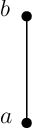
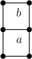
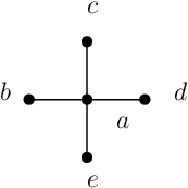
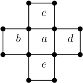
In this phase, we generate an orthogonal initial layout of $T$. For each node in $T$, we create a four-cycle. Figure 3(a) shows a tree $T$ with two nodes, $a$ and $b$. For node $a$ in the tree, we generate a four-cycle and for node $b$ we generate another four-cycle adjacent to the existing four-cycle because node $a$ is adjacent to node $b$ in the tree. The corresponding layout is shown in Figure 3(b). We define this as the initial layout. For the example tree of Figure 3(c), the corresponding initial layout is shown in Figure 3(d).

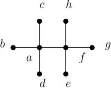
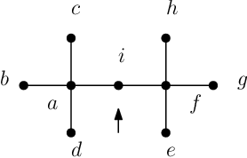
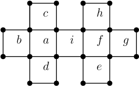
As explained in the first phase, after generating a tree, if two degree-$4$ nodes are adjacent, we insert a new node between them to separate them (see Figure 3(e), 3(f), and 3(g)). Since a four-cycle has only four sides, two degree-$4$ nodes cannot be adjacent. As we are interested in generating proper weakly chordal graphs (and not just chordal graphs), we want to have four-cycles in the initial layout. At this point, if the orthogonal layout has more than $n$ vertices, we delete vertices from four cycles to make it equal to $n$. To delete a vertex, we select vertices having degree at most two. If the number of edges in the initial layout is greater than or equal to the given $m$, the algorithm stops and returns the layout as a weakly chordal graph. Otherwise, it takes the difference of the number of edges and inserts that many edges in the initial layout to produce a weakly chordal graph. Now we denote the number of edges as $m^{\prime}$ in the initial orthogonal layout.

After generating an initial layout, we insert $(m-m^{\prime})$ edges to generate weakly chordal graphs. We divide the insertion of an edge $\{u,v\}$ into two cases. The first case considers when $I_{u,v}$ is non-empty and the second case is when $I_{u,v}$ is empty, where $I_{u,v}=N(u)\cap N(v)$, represents the set of common neighbors between $u$ and $v$. Let’s discuss the case first when $I_{u,v}$ is non-empty.

The tree generation is the first phase in the proposed approach and can be constructed in time $O(k)$ where $k$ is the number of nodes in a tree. For $k$ nodes in the tree, we insert $3k+1$ edges in the layout and each edge insertion can be done in constant time. So the initial layout can be generated in $O(k)$ time.

In the third phase, the pair of vertices $\{u,v\}$ is chosen at random to insert an edge between them. Two types of failures may arise. One is that the pair of vertices $\{u,v\}$ corresponds to an existent edge and the other is the addition of $\{u,v\}$ violates weak chordality property. To avoid the first type of failures either we can maintain a list of edges (those are present in the complement graph) not present in the current graph or we can check the existence of an edge in constant time by maintaining the adjacency matrix representation of the current graph.

Computing the neighborhood of a vertex takes linear time. Thus step 7 takes linear time. By amortizing over the edges we can see that step 8 takes linear time in the number of edges $m$ and the number of vertices $n$. Thus each of the neighborhood computations take linear time. The $AuxGraph$ can be created in linear time on the number of vertices in the $AuxNodes$. Using breadth-first search (BFS), we find whether there is a path exist between $u$ and $v$ in linear time. To find all $P_{3}$ shortest paths we also use BFS by keeping track of all predecessors between $u$ and $v$. All the operations including neighborhood computations, induced graph creations, and finding alternate longer paths take linear time (see step 23 and step 32).

For steps 25 and 34, the forbidden configuration checking is required when two or more shortest $P_{3}$ paths exist between $u$ and $v$ and the checking has to be done by considering all pairwise disjoint shortest paths. The checking is performed by the presence of one of the cross edges (an edge from one of the internal nodes from one shortest path to the alternate internal node of another shortest path) on the induced graph on a pair of disjoint shortest paths. There are at most $O(n^{3})$ pairs of mutually disjoint $P_{3}$ paths between $u$ and $v$ and thus the step takes $O(n^{3})$ time (see Appendix). We use BFS to find an alternate longer path between $u$ and $v$. Since there are at most $O(n^{2})$ multiple $P_{3}$ paths between $u$ and $v$ and thus in total we spend $O(n^{2})$ time. In the worst case, an insertion query runs in $O(n^{3})$ time.

The insertion of $\{u,v\}$ is performed in time $O(1)$ because we need to insert $u$ in the neighborhood of $v$ and $v$ in the neighborhood of $u$.

References

- [1] Srinivasa Rao Arikati and C. Pandu Rangan. An efficient algorithm for finding a two-pair, and its applications. Discrete Applied Mathematics, 31(1):71–74, 1991.
- [2] D. R. Fulkerson and O. A. Gross. Incidence matrices and interval graphs. Pacific J. Math., 15(3):835–855, 1965.
- [3] Ryan B. Hayward. Weakly triangulated graphs. J. Comb. Theory, Ser. B, 39(3):200–208, 1985.
- [4] Ryan B. Hayward. Generating weakly triangulated graphs. Journal of Graph Theory, 21(1):67–69, 1996.
- [5] Ryan B. Hayward, Chính T. Hoàng, and Frédéric Maffray. Optimizing weakly triangulated graphs. Graphs and Combinatorics, 5(1):339–349, 1989.
- [6] Lilian Markenzon, Oswaldo Vernet, and Luiz Henrique Araujo. Two methods for the generation of chordal graphs. Annals OR, 157(1):47–60, 2008.
- [7] Brendan D. McKay and Nicholas C. Wormald. Uniform generation of random regular graphs of moderate degree. J. Algorithms, 11(1):52–67, 1990.
- [8] Asish Mukhopadhyay, S. V. Rao, Sidharth Pardeshi, and Srinivas Gundlapalli. Linear layouts of weakly triangulated graphs. Discrete Math., Alg. and Appl., 8(3):1–21, 2016.
- [9] H. Prüfer. Neuer beweis eines satzes über permutationen. Arch. Math. Phys., 27:742–744, 1918.
- [10] Jeremy P. Spinrad and R. Sritharan. Algorithms for weakly triangulated graphs. Discrete Applied Mathematics, 59(2):181–191, 1995.
- [11] G. Tinhofer. Generating Graphs Uniformly at Random, pages 235–255. Springer Vienna, Vienna, 1990.
- [12] Nicholas C. Wormald. Generating random regular graphs. J. Algorithms, 5(2):247–280, 1984.
- [13] Nicholas C. Wormald. Generating random unlabelled graphs. SIAM J. Comput., 16(4):717–727, 1987.