A library to compute the density of the distance between a point and a random variable uniformly distributed in some sets
Abstract.
In [2], algorithms to compute the density of the
distance to a random variable uniformly distributed in (a) a ball, (b) a disk, (c) a line
segment, or (d) a polygone were introduced.
For case (d), the algorithm, based on Green’s theorem,
has complexity log() where is the number of
vertices of the polygone.
In this paper, we present for case (d) another algorithm with the same complexity, based on a triangulation
of the polygone. We also describe an open source library, available at https://github.com/vguigues/Areas_Library,
providing this algorithm as well as the
algorithms from [2].
Vincent Guigues
School of Applied Mathematics, FGV
Praia de Botafogo, Rio de Janeiro, Brazil
vguigues@fgv.br
Keywords: Computational Geometry, Geometric Probability, Distance to a random variable, Uniform distribution, Green’s theorem, PSHA.
MSC2010 subject classifications: 60D05, 65D99, 51N20, 65D30, 86A15.
1. Introduction
Let be a closed and bounded set and let be a random variable uniformly distributed in . Given , consider random variable given by the Euclidean distance between and , i.e., for any .
Denoting respectively the density and the cumulative distribution function (CDF) of by and , we have if while and if . For , we have
where is the Lebesgue measure of the set and is the ball of center and radius . As a result, the computation of the CDF of amounts to the problem of computing the Lebesgue measures of and of for any .
When is a disk, a ball, or a line segment, it is easy to derive analytic expressions for both the CDF and the density of , see [2] for details. When is a polygone, an algorithm based on Green’s theorem computing exactly the CDF of is described in [2].
The study of these four cases is useful for Probabilistic Seismic Hazard Analysis (PSHA) to obtain the distribution of the distance between a given location on earth and the epicenter of an earthquake which, in a given seismic zone, is usually assumed to have a uniform distribution in that zone modelled as a union of disks, a union of balls, a union of line segments, or the boundary of a polyhedron in . This application, which motivated this study, is described in Section 2 of [2], following the lines of the seminal papers [1], [3], which paved the way for PSHA.
In this paper, we describe in Section 2 an algorithm to compute the CDF of when is a polygone using a triangulation of the polygone. This amounts to computing the area of the intersection of a disk and a triangle. To solve this problem, we enumerate all possible shapes for this intersection, identify in which of these cases we are (using tests depending on the disk and triangle considered), and compute the area of this shape. This shape can be decomposed as a union of triangles and lenses and therefore its area can be easily computed analytically. Finally, in Section 3, we describe the main functions of an open source library, available at https://github.com/vguigues/Areas_Library, implementing the algorithms from [2] and Section 2.
Throughout the paper, we use the following notation. For a point in , we denote its coordinates with respect to a given Cartesian coordinate system by and . For two points , is the line segment joining points and , i.e., , is the line passing through and , and is the vector whose coordinates are . Given two vectors , we denote the usual scalar product of and in by . For , we denote the circle and the disk of center and radius by respectively and .
2. An algorithm based on a triangulation of the polygone
Let be a simple polygone contained in a plane given by its extremal points where the boundary of is where for and .
The computation, at a given value , of the CDF of the distance between a given point and requires computing the area of the intersection of and of the ball of center and radius . Without loss generality, we will assume that is in the plane containing (if this is not the case, we can project onto this plane and modify the value of the radius, see [2] for details). The area of the intersection can be obtained computing a triangulation of the polyhedron (with complexity ), then computing the area of intersection of disk with the triangles of the triangulation, and summing these areas. Therefore, we need to devise an algorithm to compute the area of the intersection of a disk and a triangle and we proceed as follows.
Consider a triangle with vertices and a disk of center and radius . We want to compute the area of the intesection of this triangle and this disk.
We first compute:
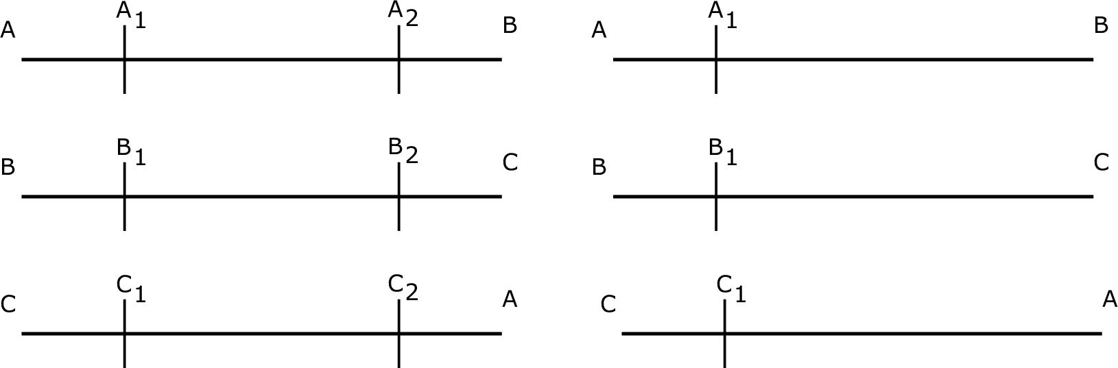
Each , can take 3 values (, or )
and therefore the triple can take
27 possible different values.
We associate to base 3 number its decimal
equivalent, denoted by Code in what follows,
and given by .
To identify the shape of the intersection between the triangle
and the disk, we branch according to the value of
variable Code and for a given value of Code,
we consider all possible shapes for the intersection of the triangle
and the disk. Obviously, for
all values of Code corresponding
to different permutations of the same triple
the different possible shapes for the intersection are the same.
We now discuss for every possible value of variable
Code how to compute the area of the intersection.
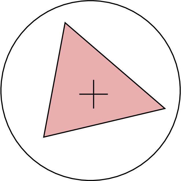
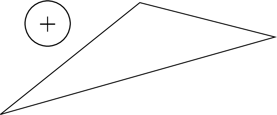
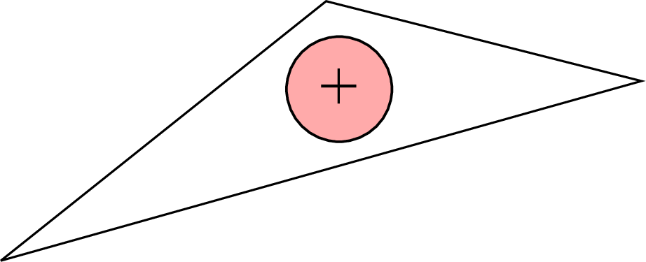
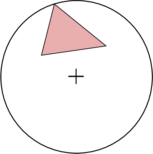
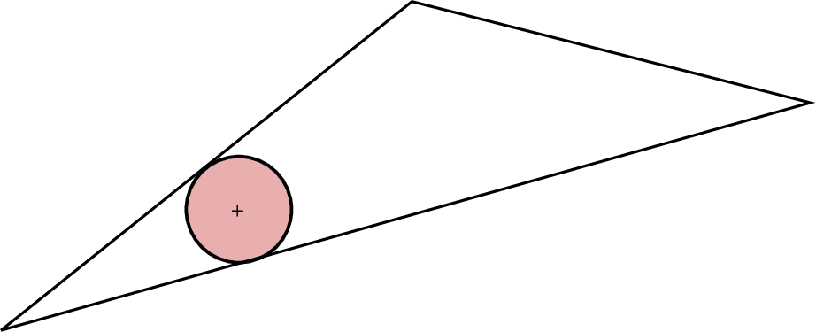
In this case, there is no intersection between the circle and the triangle. There are three possible shapes for the intersection represented in Figure 2: (a) the triangle is contained in the disk, (b) the disk is outside the triangle, and (c) the disk is inside the triangle.
 |
 |
 |
| (a) | (b) | (c) |
To know which of subcases (a), (b), or (c) we are in, we compute
| (2.1) |
In what follows, we denote by
| (2.2) |
the area of triangle .
If , and then
the area is . Otherwise
either is inside the triangle and the area
is or it is outside and the area is null.
To know if is inside or outside the triangle,
we compute the crossing number for and the triangle
(see [4] for the definition of the crossing number
and for instance [2, 4] for an algorithm to compute it) and the minimal distance from to the border
of the triangle.
Knowing that the crossing number is odd if and only if
belongs to the relative interior of the triangle,
is inside the triangle
if and only if or the crossing
number is odd.
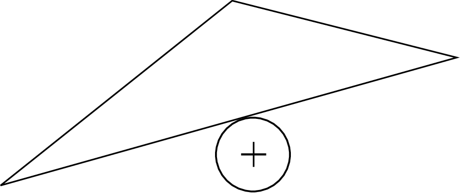
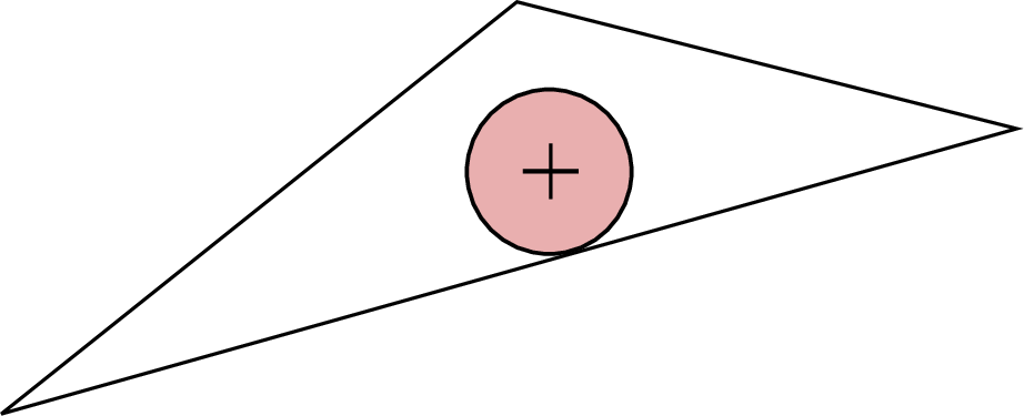
, corresponding
to , i.e., one side
of the triangle has a single intersection with the circle
and the remaining two have no intersection.
There are two possible shapes for the intersection represented in Figure 3-(a),(b).
 |
 |
| (a) | (b) |
In case (a), is outside the triangle and the area is null while in
case (b), is inside the triangle and the area is . We have already seen how
to differentiate these two cases on the basis of and of the
crossing number.
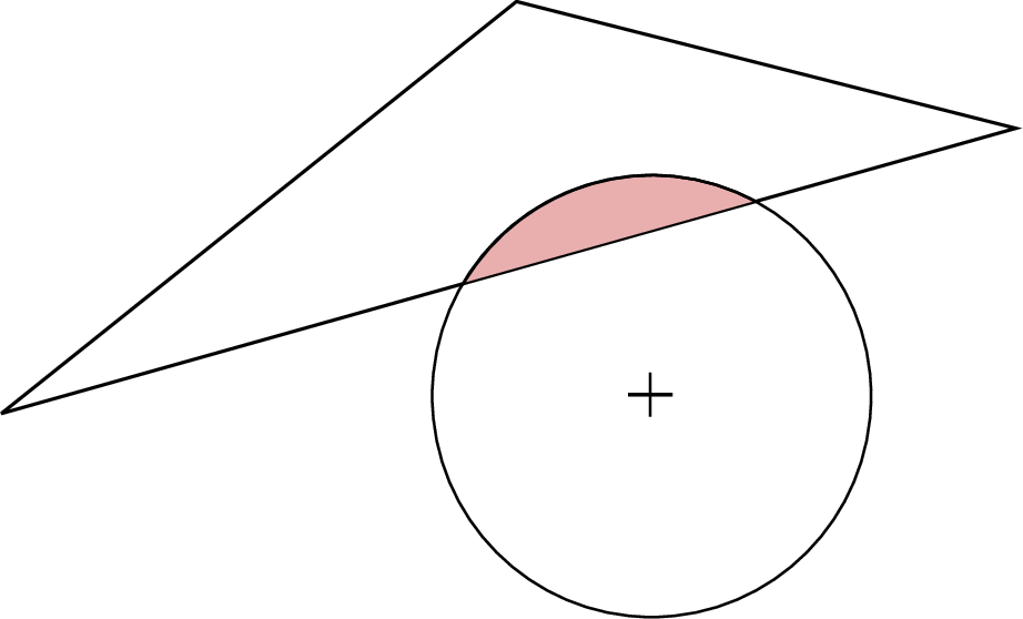
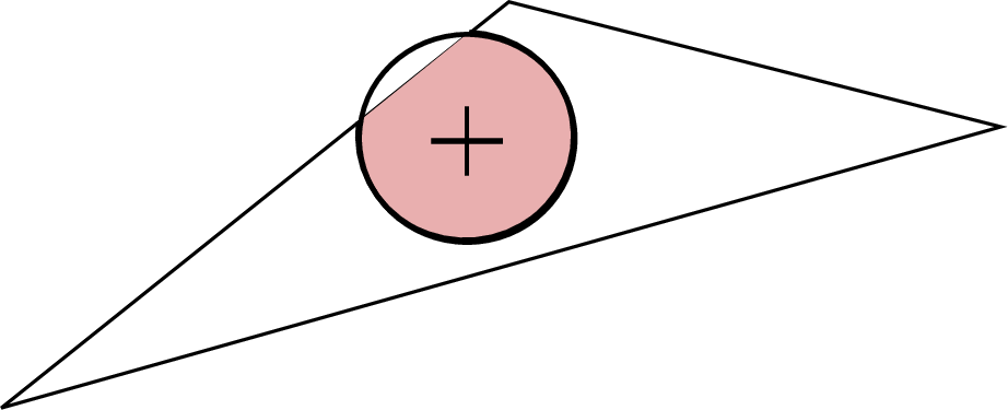
obtained when is
, respectively.
There are two possible shapes for the intersection represented in Figure 4-(a), (b).
 |
 |
| (a) | (b) |
In each case, the intersection is a lens, of area in case (a) and in case (b). Let us recall how to compute analytically these areas.
Consider a chord of circle . It defines two lenses represented in Figure 5-(a), (b).
 |
 | |
| (a) | (b) |
Let us recall the formula for the area of the lens in case (a) (in case (b), it is given by ). In case (a), let and let be the cosine of acute angle given by
Then
With this notation, when , i.e., when
, in case (a), the area of the intersection is
given by .
The cases where are dealt with by appropriate permutation
of the intersection points.
obtained when
is , , .
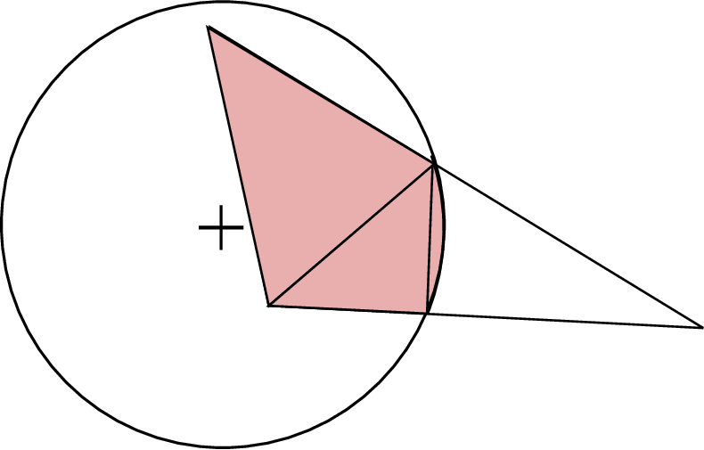
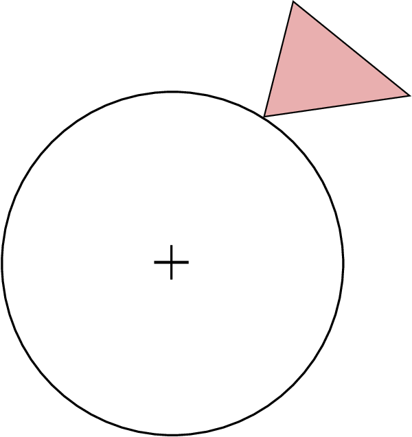
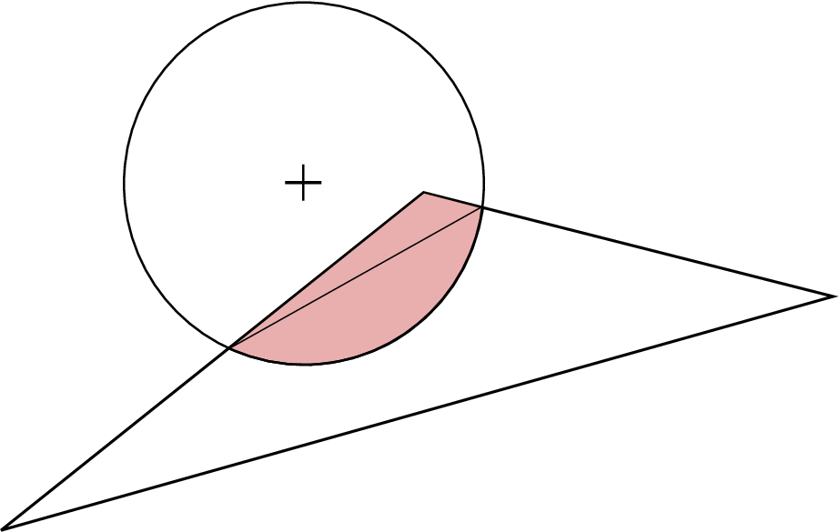
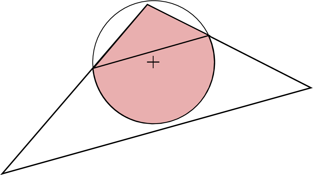
The possible shapes for the intersection between the triangle and disk are given in Figure 6.
 |
 |
| (a) | (b) |
 |
 |
| (c) | (d) |
 |
 |
| (e) | (f) |
We discuss how to compute the intersection area when , i.e., . The cases Code=4,10, are similar, obtained by appropriate permutation of and the intersection points.
Let us first discuss on how to distinguish between cases (e) and (f). In theses cases, the intersection is the union of a triangle and a lens. In case (e) the lens has area lower than or equal to while in case (f) the lens has area greater than . In case (f), and are in two different half-spaces separated by line . More precisely, let us introduce the function
[out]=Are_In_Same_Half_Space(C,P,A,B)
with inputs four points in which returns 0 if and are in two different half-spaces separated by line and 1 otherwise. Clearly, out is 1 if and only if ( and ) or ( and ) where
With this notation, the intersection area in cases (a)-(f) is
computed with the following pseudo-code where area
will store the intersection area:
area=0.
if and and then
else if and , and then
else if and and then
else if and and then
[out]=Are_In_Same_Half_Space,
if out=1 then area,
else area,
end if
end if
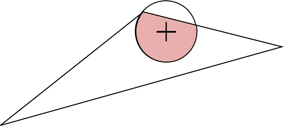
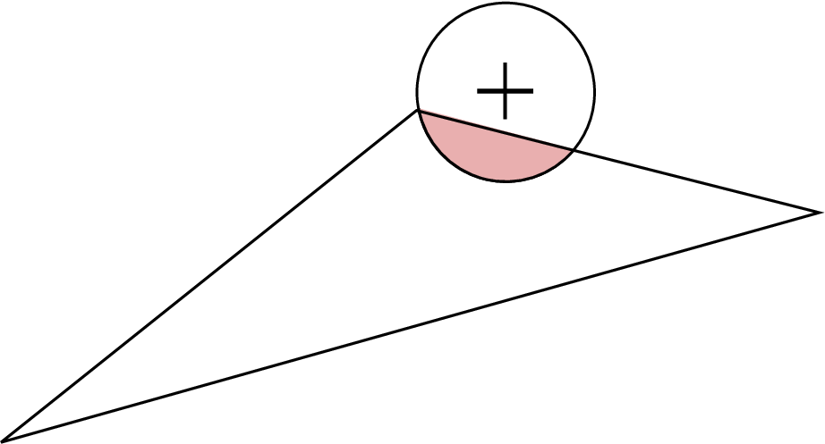
corresponding to ,
,, , ,
.
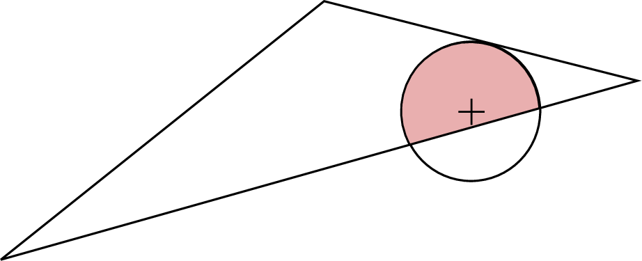
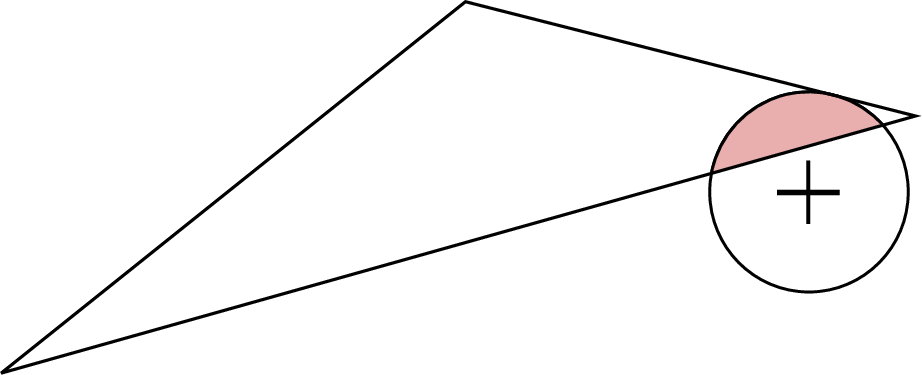
The possible shapes for the intersection are represented in Figure 7.
 |
 |
| (a) | (b) |
 |
 |
| (c) | (d) |
It follows that
when Code=5 or 11, i.e., when
is
or , the area of the intersection
is computed with the following pseudo-code (stored
in variable area):
if the crossing number for and the triangle is odd or then area
else area=.
end if
The pseudo-codes when Code=7,15,19,21,
are obtained by appropriate permutations of
the intersection points.
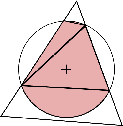
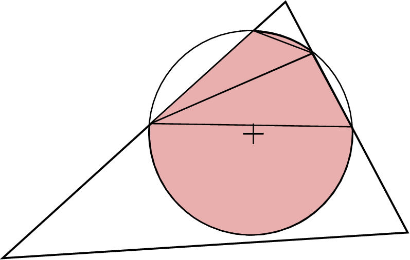
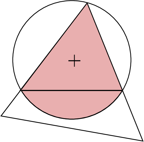
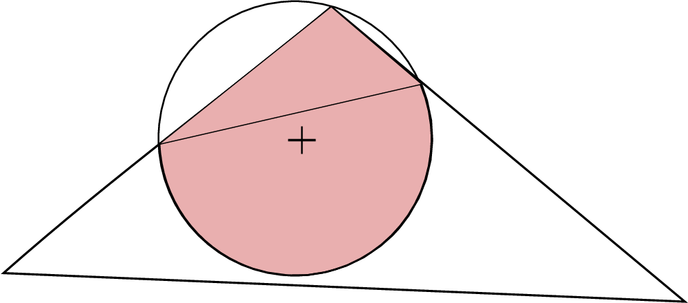
obtained when , , .
The possible shapes for the intersection are represented in Figure 8.
 |
 | |
| (a) | (b) | |
 |
 | |
| (c) | (d) |
It follows that when Code=8, i.e., when
the pseudo-code for computing the
area of the intersection (stored in variable area)
is the following:
area=0.
[out]=Are_In_Same_Half_Space
if
if out=1
area= ,
else
area= ,
end if
else
if out=1
area= ,
else
area= .
end if
end if
The pseudo-codes for
Code and
are obtained by appropriate permutations of
, and the intersection points.
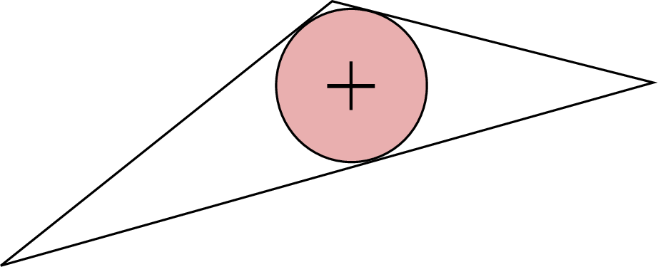
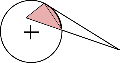
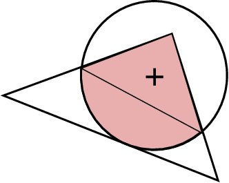
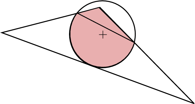
obtained when
.
The possible shapes for the intersection are represented in Figure 9.
 |
 | |
| (a) | (b) | |
 |
 | |
| (c) | (d) |
Therefore the pseudo-code for computing the intersection
area is the following (where
the area of the intersection is stored in variable area):
if and and then
else if and and then
else if and and then
else if and and then
else if and and then
else if and and then
else if and and then
else if and and then
[out]=Are_In_Same_Half_Space,
if out=1 then area,
else area
end if
else if and and then
[out]=Are_In_Same_Half_Space,
if out=1 then area,
else area
end if
else if and and then
[out]=Are_In_Same_Half_Space,
if out=1 then area,
else area,
end if
end if
obtained when . The possible shapes for the intersection are represented in Figure 10.
|
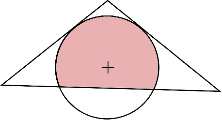
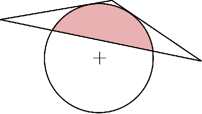
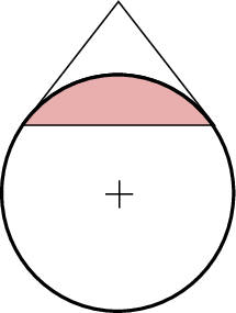
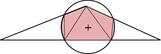
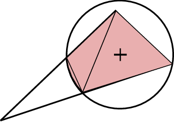
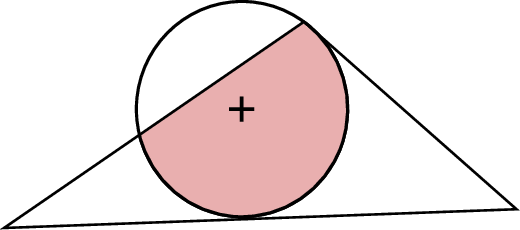
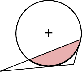
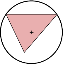
It follows that the pseudo-code for computing the area of the intersection
(stored in variable area) when Code
is the following:
area.
if and and then
[out]=Are_In_Same_Half_Space,
if out=1 then area,
else area,
end if
else if and and then
area,
else if and and then area,
else if and and then area,
else if
if then area,
else
[out]=Are_In_Same_Half_Space,
if out then area,
else area,
end if
end if
else if
if then area,
else
[out]=Are_In_Same_Half_Space,
if out then area,
else area,
end if
end if
end if
The pseudo-codes when
Code and are
obtained
by appropriate permutation of ,
and the intersection points.
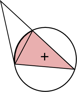
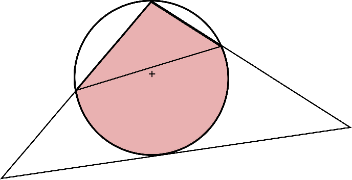
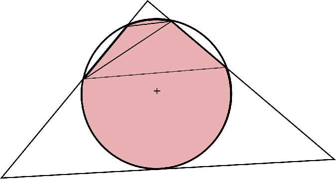
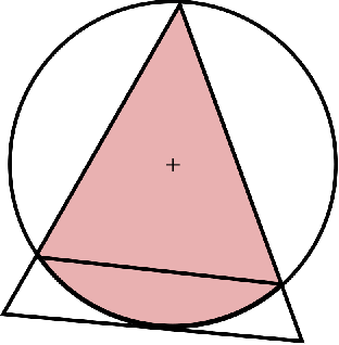
obtained when . The possible shapes for the intersection are represented in Figure 11.
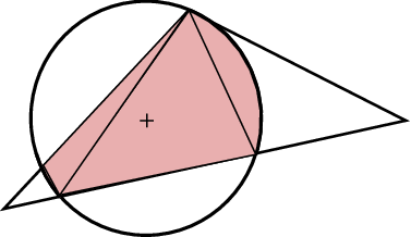 |
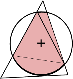 | |
| (a) | (b) | |
 |
 | |
| (c) | (d) | |
 |
 | |
| (e) | (f) |
It follows that when Code the pseudo-code
for computing the area of the intersection is the
following:
if and and then
[out]=Are_In_Same_Half_Space,
if out then area,
else area,
end if
else if and then area,
else if and then area,
else if then
[out]=Are_In_Same_Half_Space,
if out then area,
else area,
end if
else if then
else if then
end if.
The pseudo-codes when
Code and are
obtained
by appropriate permutation of ,
and the intersection points.
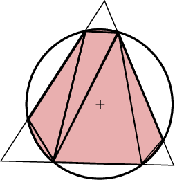
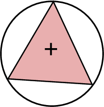
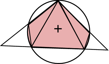
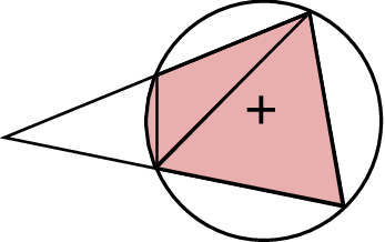
corresponding to . The possible shapes for the intersection are represented in Figure 12.
 |
 | |
| (a) | (b) | |
 |
 | |
| (c) | (d) |
From this figure we obtain the following pseudo-code to compute the intersection area:
if and and then
else if and and then area,
else if and and then
else if and and then
else if and and then
else if and and then
else if and and then
else if and and then
end if
3. The library: main functions and examples
The Matlab library, available at https://github.com/vguigues/Areas_Library, computes the density of the distance to a random variable uniformly distributed in some sets and the area of intersection of disks and balls with those sets.
All necessary files to run the functions of the library are in folders Areas_Library and its subfolder Examples which contains files to run the main functions on examples. No external library is needed. We implemented all functions of these folders except function polygon_triangulate which computes a triangulation of a polygone. This function, which can be found in folder Areas_Library, is the Matlab version by John Burkardt of the original C version by Joseph ORourke [4].
If the folder Areas_Libary is copied in folder
C:\Users\user_name, before using the library, update the path in Matlab with commands:
addpath ’C:\Users\user_name\Areas_Libary’
addpath ’C:\Users\user_name\Areas_Libary\Examples’
The next section shows how to use the main functions of the library using the files of examples that can be found in folder Areas_Libary\Examples.
3.1. Density of the distance to a random variable uniformly distributed in a polygone
The function to compute the density of the distance from a point
to a random variable uniformly distributed in a polygone is:
[d,time,dmin,dmax]=density_polyhedron(S,P,Np,algo)
where input variables are:
- •
- •
Np: the number of discretization points: the density is computed at Np equally spaced points from the support of the random variable distance.
- •
: point as explained above.
- •
: the polyhedron where is the number of vertices and are the successive vertices of the polyhedron. Observe that the first point is repeated. When algo=’g’, when travelling on the boundary of from to , then from to and so on until the last line segment , one always has the relative interior of to the left. When algo=’t1’ this restriction does not apply: if algo=’t1’, when travelling on of from to , then from to and so on until the last line segment , one can either have the relative interior of to the left or to the right.
Output variables of function density_polyhedron are:
- •
d: a vector of size Np where is the estimation of the density of the random variable at .
- •
time is the time required to compute .
- •
]dmin,dmax[ is the support of the random variable meaning that dmax is the maximal distance between and the boundary of the polygone. If is inside the polygone then dmin and if is outside the polygone then dmin is the minimal distance from to the boundary of the polygone.
We illustrate the use of this function on several examples written in folder ’Areas_Libary\Examples’.
We start with an example written in file drectex.m of folder Examples where is a rectangle with side lengths and with and is the center of the rectangle. For this example, the density of the distance from to a random variable uniformly distributed in is known in closed form and is given in [5]. Therefore, this example allows us to test the implementation of function density_polyhedron comparing output d of this function when algo=’g’, ’t1’ with the theoretical values given in [5].
The function corresponding to this example is
[dG,dT1,d,ErrG,ErrT1]=drectex(Np,,).
The input variables are parameters Np, , given above and the outputs are the following:
- •
dG and dT1 are vectors of size Np and dG (resp. dT1) is the value of the density at Np, computed calling function density_polyhedron with variable algo=’g’ (resp. calling function density_polyhedron with variable algo=’t1’). Recall that are Np equally spaced points in ]dmin,dmax[.
- •
d is a vector of size Np: d is the exact value of the density at computed using the analytic formulas given in [5].
- •
ErrG is the maximal error when algo=’g’, i.e., ErrG.
- •
ErrT1 is the maximal error when algo=’t1’, i.e., ErrT1.
On top of that, the function plots
vectors dG, dT1, and d.
For instance, running
[dG,dT1,d,ErrG,ErrT1]=drectex(1,0.8,1).
the plots of Figure 13 are displayed. On this Figure, from left to right, the first plot represents rectangle and , the second plot represents the density of obtained using the algorithm from [2], the third plot is the density of obtained using the algorithm from Section 2, while the last plot is the graph of the true density of .

In this example, the densities are computed with the following Matlab code:
P1=[0,0]; P2=[L,0]; P3=[L,alphaL]; P4=[0,alphaL];
P=[L/2,alphaL/2];
S=[P1;P2;P3;P4;P1];
[dG,timeg,dmin,dmax]=density_polyhedron(S,P,Nb,’g’);
[dT1,timet1,dmin,dmax]=density_polyhedron(S,P,Nb,’t1’);
ErrG=max(abs(d-dG)); ErrT1=max(abs(d-dT1)).
To check the implementations of the algorithm from [2] and the algorithm from Section 2, we now report in Table 1 the values of ErrG and ErrT1 for several values of the number Np of discretization points, namely when Np varies in the set .
| Np | ErrG | ErrT1 |
|---|---|---|
| 0.017 | 0.023 | |
| 0.010 | 0.020 | |
| 0.007 | 0.04 | |
| 0.004 | 0.03 |
In all cases the maximal error is very small which shows that
both algorithms correctly compute
the Np areas of intersection of the disks and polygone of this
example.11
1
To approximate the density at
Np points, we need to compute the cumulative distribution function
at Np points and therefore when
Np, the algorithms
are called times each to compute areas.
We also observe that the approximations are slightly better with
the algorithm from [2] and, as expected, the maximal error decreases with
Np for this algorithm. This is not the case for the other, probably
due to roundoff errors.
We now compare the algorithms
on other examples coded in Matlab file dpolyex.m.
More precisely, we consider three polyhedra
(a triangle, a rectangle, and an arbitrary polygone)
and in each case a point
inside the polygone and a point outside.
For these 6 examples the Matlab codes are the following.
is a triangle and is outside this triangle. In Figure 14, and are represented in the left plot while the corresponding density of is represented in the right plot.
This density is obtained with the following Matlab code:
P1=[1,1]; P2=[10,1]; P3=[3,4]; S=[P1;P2;P3;P1]; P=[5,0];
[dT1,timeT1,dminT1,dmaxT1]=density_polyhedron(S,P,Np,algo);
where algo=’g’ or ’t1’.
is a triangle and is inside this triangle. In Figure 15, and are represented in the left plot while the corresponding density of is represented in the right plot.
This density is obtained with the following Matlab code:
P1=[1,1]; P2=[10,1]; P3=[3,4]; S=[P1;P2;P3;P1];; P=[4,2];
[dT2,timeT2,dminT2,dmaxT2]=density_polyhedron(S,P,Np,algo);
where algo=’g’ or ’t1’.
is a rectangle and is outside this rectangle. In Figure 16, and are represented in the left plot while the corresponding density of is represented in the right plot.
This density is obtained with the following Matlab code:
P1=[3,3]; P2=[12,3]; P3=[12,7]; P4=[3,7]; S=[P1;P2;P3;P4;P1]; P=[1,1];
[dR1,timeR1,dminR1,dmaxR1]=density_polyhedron(S,P,Np,algo);
where algo=’g’ or ’t1’.
is a rectangle and is inside this rectangle. In Figure 17, and are represented in the left plot while the corresponding density of is represented in the right plot.
This density is obtained with the following Matlab code:
P1=[3,3]; P2=[12,3]; P3=[12,7]; P4=[3,7]; S=[P1;P2;P3;P4;P1]; P=[6,5];
[dR2,timeR2,dminR2,dmaxR2]=density_polyhedron(S,P,Np,algo);
where algo=’g’ or ’t1’.
is a polygone and is outside this polygone. In Figure 18, and are represented in the left plot while the corresponding density of is represented in the right plot.
This density is obtained with the following Matlab code:
P1=[1,1]; P2=[3,1]; P3=[5,2]; P4=[7,1]; P5=[8,3];
P6=[6,3]; P7=[7,6]; P8=[4,5]; P9=[1,3]; P10=[2,2];
S=[P1;P2;P3;P4;P5;P6;P7;P8;P9;P10;P1];
P=[4,0];
[dP1,timeP1,dminP1,dmaxP1]=density_polyhedron(S,P,Np,algo);
where algo=’g’ or ’t1’.
is a polygone and is inside this polygone. In Figure 19, and are represented in the left plot while the corresponding density of is represented in the right plot.
This density is obtained with the following Matlab code:
P1=[1,1]; P2=[3,1]; P3=[5,2]; P4=[7,1]; P5=[8,3];
P6=[6,3]; P7=[7,6]; P8=[4,5]; P9=[1,3]; P10=[2,2];
S=[P1;P2;P3;P4;P5;P6;P7;P8;P9;P10;P1];
P=[4,3];
[dP2,timeP2,dminP2,dmaxP2]=density_polyhedron(S,P,Np,algo);
where algo=’g’ or ’t1’.
Command
[dT1,dT2,dR1,dR2,dP1,dP2]=dpolyex(10 000,’g’)
will run the code above to compute dT1,dT2,dR1,dR2,dP1,dP2
with algo=’g’, Np, and will
produce Figure 20 which represents polygones
above and the corresponding densities of on their right.

Command
[dT1,dT2,dR1,dR2,dP1,dP2]=dpolyex(Np,’t1’)
does the same with algo=’t1’.
Let (resp. ) be the approximation of the density computed by the algorithm from [2] based on Green’s theorem (resp. the algorithm from Section 2, based on a triangulation of the polygone) at . The maximal errors were for given in Figure 14, for given in Figure 15, for given in Figure 16, for given in Figure 17, for given in Figure 18, and for given in Figure 19.
The fact that these errors are very small is an indication that both algorithms were correctly implemented.
3.2. Area of the intersection of a disk and a polygone
The area of the intersection of polygone
(in Matlab notation)
and the disk of center and radius is computed as follows
with the library:
[Crossing_Number,AreaP,dmin,dmax]=polyhedron(S,P,n)
[area]=area_intersection_disk_polygone(S,P,d,n,Crossing_Number,AreaP,algo)
where output area of function area_intersection_disk_polygone is the area of the intersection and the outputs of the first function polyhedron are:
- •
Crossing_Number: the crossing number for and ;
- •
AreaP: the area of polygone ;
- •
dmin (resp. dmax): the minimal (resp. maximal) distance from to the border of the polygone.
When algo=’g’ (resp. ’t1’) the area of the intersection is computed with the algorithm described in [2] (resp. the algorithm given in Section 2).
We test this function computing the
areas of intersection of 350 disks and polygones as well
as the mean and maximal time required to compute these areas.
The polygones are generated using function
[Polygone]=generate_polygone(n,)
of the library where parameters and are described below. This function generates randomly a polygone with vertices as follows. We sample points taking points in each orthant with polar angles generated randomly and independently in this orthant and radial coordinates generated randomly and independently in the interval [0,] (we take in our experiments). We then sort in ascending order the polar angles of these points. This list defines the successive vertices of a star-shaped (simple) polygone. The coordinates of the centers of the disks (resp. the radii) are obtained sampling independently from the uniform distribution on the interval (resp. ).
For each value of in the set
we generate 50 star-shaped polyhedra and disks as explained above and for each polygone
and disk, we compute the area of their intersection using
both algorithms.
The corresponding function of the library is
[Errmax,ErrMoy,TimeGreen,TimeTr1]=random_areas()
where is the number of Monte-Carlo simulations ( in our experiments) and where the outputs are the following:
- •
TimeGreen(k,j) (resp. TimeTr1(k,j) is the time required to compute the intersection area for -th instance and -th value of (for instance for we have , for , we have ) when area_intersection_disk_polygone is called with algo=’g’ (resp. algo=’t1’);
- •
Errmax and ErrMoy are vectors of size . ErrMoy and Errmax are defined respectively by and where and are the areas of the intersection for -th Monte-Carlo simulation and -th value of computed with respectively algo=’g’ and algo=’t1’.
For each value of , the mean and maximal time (over the 50 instances) required to compute these areas are reported in Table 2. We also report in this table the values of Errmax and ErrMoy.
|
|
|
|
ErrMoy | Errmax | |||||||||
|---|---|---|---|---|---|---|---|---|---|---|---|---|---|---|
| 40 | 0.30 | 0.004 | 0.34 | 0.008 | 9.5 | |||||||||
| 100 | 1.99 | 0.007 | 2.54 | 0.014 | 2.5 | 4.1 | ||||||||
| 200 | 8.09 | 0.012 | 8.96 | 0.018 | 3.8 | 3.6 | ||||||||
| 320 | 22.57 | 0.020 | 34.26 | 0.036 | 6.8 | 3.4 | ||||||||
| 400 | 45.21 | 0.021 | 669.76 | 0.039 | 1.1 | 1.7 | ||||||||
| 600 | 128.52 | 0.033 | 2 772.5 | 0.074 | 1.4 | 1.2 | ||||||||
| 800 | 369.80 | 0.043 | 9 661.8 | 0.076 | 1.7 | 9.7 |
We observe that errors are negligible which shows that both algorithms compute
the same areas. Moreover, on all instances
algorithm from [2] computes all areas
extremely quickly and much quicker than
the algorithm of Section 2.
For this latter algorithm, both the mean
and maximal time required to compute the intersection areas significantly increase
with the number of vertices of the polygone.
Acknowledgments The author’s research was partially supported by an FGV grant, CNPq grant 307287/2013-0, and FAPERJ grants E-26/110.313/2014 and E-26/201.599/2014.
References
- [1] C.A. Cornell. Engineering seismic risk analysis. Bull. Seism. Soc. Am., 58:1583–1606, 1968.
- [2] V. Guigues. Computation of the cumulative distribution function of the Euclidean distance between a point and a random variable uniformly distributed in disks, balls, or polyhedrons and application to Probabilistic Seismic Hazard Analysis. arXiv, 2015. https://arxiv.org/abs/1809.02007.
- [3] R.K. McGuire. Fortran computer program for seismic risk analysis. US Geological Survey Open-File Report, Series Number: 76-67, 1976.
- [4] J. O’Rourke. Computational Geometry in C. Cambridge University Press New York, NY, USA, 1998.
- [5] R. Stewart and H. Zhang. A note concerning the distances of uniformly distributed points from the centre of a rectangle. Bull. Aust. Math. Soc., 87:115–119, 2013.