Deep ReLU Networks Have
Surprisingly Few Activation Patterns
Abstract
The success of deep networks has been attributed in part to their expressivity: per parameter, deep networks can approximate a richer class of functions than shallow networks. In ReLU networks, the number of activation patterns is one measure of expressivity; and the maximum number of patterns grows exponentially with the depth. However, recent work has showed that the practical expressivity of deep networks – the functions they can learn rather than express – is often far from the theoretical maximum. In this paper, we show that the average number of activation patterns for ReLU networks at initialization is bounded by the total number of neurons raised to the input dimension. We show empirically that this bound, which is independent of the depth, is tight both at initialization and during training, even on memorization tasks that should maximize the number of activation patterns. Our work suggests that realizing the full expressivity of deep networks may not be possible in practice, at least with current methods.
1 Introduction
A fundamental question in the theory of deep learning is why deeper networks often work better in practice than shallow ones. One proposed explanation is that, while even shallow neural networks are universal approximators [3, 9, 12, 20, 27], there are functions for which increased depth allows exponentially more efficient representations. This phenomenon has been quantified for various complexity measures [6, 7, 8, 13, 24, 25, 28, 29, 30, 31]. However, authors such as Ba and Caruana have called into question this point of view [2], observing that shallow networks can often be trained to imitate deep networks and thus that functions learned in practice by deep networks may not achieve the full expressive power of depth.
In this article, we attempt to capture the difference between the maximum complexity of deep networks and the complexity of functions that are actually learned (see Figure 1). We provide theoretical and empirical analyses of the typical complexity of the function computed by a ReLU network . Given a vector of its trainable parameters, computes a continuous and piecewise linear function . Each thus is associated with a partition of input space into activation regions, polytopes on which computes a single linear function corresponding to a fixed activation pattern in the neurons of
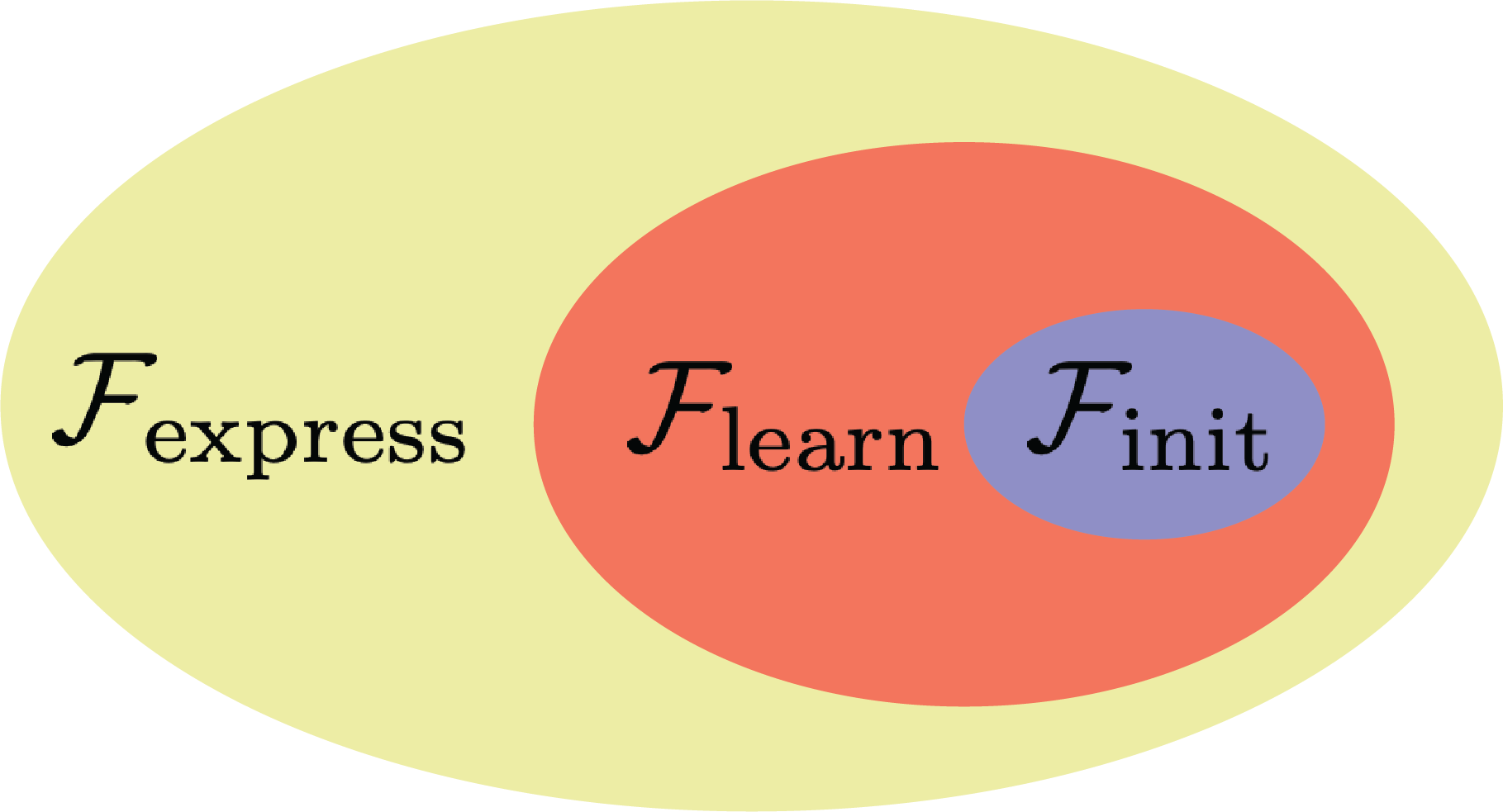
We aim to count the number of such activation regions. This number has been the subject of previous work (see §1.1), with the majority concerning large lower bounds on the maximum over all of the number of regions for a given network architecture. In contrast, we are interested in the typical behavior of ReLU nets as they are used in practice. We therefore focus on small upper bounds for the average number of activation regions present for a typical value of . Our main contributions are:
- •
We give precise definitions and prove several fundamental properties of both linear and activation regions, two concepts that are often conflated in the literature (see §2).
- •
We prove in Theorem 5 an upper bound for the expected number of activation regions in a ReLU net . Roughly, we show that if is the input dimension and is a cube in input space , then, under reasonable assumptions on network gradients and biases,
(1) - •
- •


Our results show both theoretically and empirically not only that the number of activation patterns can be small for a ReLU network but that it typically is small both at initialization and throughout training, effectively capped far below its theoretical maximum even for tasks where a higher number of regions would be advantageous (see §4). We provide in §3.2-3.3 two intuitive explanations for this phenomenon. The essence of both is that many activation patterns can be created only when a typical neuron in turns on/off repeatedly, forcing the value of its pre-activation to cross the level of its bias many times. This requires (i) significant overlap between the range of on the different activation regions of and (ii) the bias to be picked within this overlap. Intuitively, (i) and (ii) require either large or highly coordinated gradients. In the former case, oscillates over a large range of outputs and can be random, while in the latter may oscillate only over a small range of outputs and is carefully chosen. Neither is likely to happen with a proper initialization. Moreover, both appear to be difficult to learn with gradient-based optimization.
The rest of this article is structured as follows. Section 2 gives formal definitions and some important properties of both activation regions and the closely related notion of linear regions (see Definitions 1 and 2).Section 3 contains our main technical result, Theorem 5, stated in §3.1. Sections 3.2 and 3.3 provide heuristics for understanding Theorem 5 and its implications. Finally, §4 is devoted to experiments that push the limits of how many activation regions a ReLU network can learn in practice.
1.1 Relation to Prior Work
We consider the typical number of activation regions in ReLU nets. In contrast, interesting bounds on the maximum number of regions are given in [6, 8, 25, 28, 29, 31, 32, 34]. Such worst case bounds are used to control the VC-dimension of ReLU networks in [4, 5, 18] but differ dramatically from our average case analysis.
Our main theoretical result, Theorem 5, is related to [17], which conjectured that our Theorem 5 should hold and proved bounds for other notions of average complexity of activation regions. Theorem 5 is also related in spirit to [10], which uses a mean field analysis of wide ReLU nets to show that they are biased towards simple functions. Our empirical work (e.g. §4) is related both to the experiments of [26] and to those of [1, 36]. The last two observe that neural networks are capable of fitting noisy or completely random data. Theorem 5 and experiments in §4 give a counterpoint, suggesting limitations on the complexity of random functions that ReLU nets can fit in practice (see Figures 4-6).


2 How to Think about Activation Regions
Before stating our main results on counting activation regions in §3, we provide a formal definition and contrast them with linear regions in §2.1. We also note in §2.1 some simple properties of activation regions that are useful both for understanding how they are built up layer by layer in a deep ReLU net and for visualizing them. Then, in §2.2, we explain the relationship between activation regions and arrangements of bent hyperplanes (see Lemma 4).
2.1 Activation Regions vs. Linear Regions
Our main objects of study in this article are activation regions, which we now define.
Definition 1 (Activation Patterns/Regions).
Let be a ReLU net with input dimension . An activation pattern for is an assignment to each neuron of a sign:
Fix , a vector of trainable parameters in , and an activation pattern The activation region corresponding to is
where neuron has pre-activation , bias and post-activation We say the activation regions of at are the non-empty activation regions .
When specifying an activation pattern , the sign assigned to a neuron determines whether is on or off for inputs in the activation region since the pre-activation of neuron is positive (resp. negative) when (resp. ). Perhaps the most fundamental property of activation regions is their convexity.
Lemma 1 (Convexity of Activation Regions).
Let be a ReLU net. Then for every activation pattern and any vector of trainable parameters for each activation region is convex.
We note that Lemma 1 has been observed before (e.g. Theorem 2 in [29]), but in much of the literature the difference between linear regions (defined below), which are not necessarily convex, and activation regions, which are, is ignored. It turns out that Lemma 1 holds for any piecewise linear activation, such as leaky ReLU and hard hyperbolic tangent/sigmoid. This fact seems to be less well-known (see Appendix B.1 for a proof). To provide a useful alternative description of activation regions for a ReLU net a fixed vector of trainable parameters and neuron of , define
| (2) |
The sets can be thought of as “bent hyperplanes” (see Lemma 4). The non-empty activation regions of at are the connected components of with all the bent hyperplanes removed:
Lemma 2 (Activation Regions as Connected Components).
For any ReLU net and any vector of trainable parameters
| (3) |
We prove Lemma 2 in Appendix B.2. We may compare activation regions with linear regions, which are the regions of input space on which the network defines different linear functions.
Definition 2 (Linear Regions).
Let be a ReLU net with input dimension , and fix , a vector of trainable parameters for . Define
The linear regions of at are the connected components of input space with removed:
Linear regions have often been conflated with activation regions, but in some cases they are different. This can, for example, happen when an entire layer of the network is zeroed out by ReLUs, leading many distinct activation regions to coalesce into a single linear region. It can also occur for non-generic configurations of weights and biases where the linear functions computed in two neighboring activation regions happen to coincide. However, the number of activation regions is always at least as large as the number of linear regions.
Lemma 3 (More Activation Regions than Linear Regions).
Let be a ReLU net. For any parameter vector for the number of linear regions in at is always bounded above by the number of activation regions in at In fact, the closure of every linear region is the closure of the union of some number of activation regions.
Lemma 3 is proved in Appendix B.3. We prove moreover in Appendix B.4 that generically, the gradient of is different in the interior of most activation regions and hence that most activation regions lie in different linear regions. In particular, this means that the number of linear regions is generically very similar to the number of activation regions.
2.2 Activation Regions and Hyperplane Arrangements
Activation regions in depth ReLU nets are given by hyperplane arrangements in (see [33]). Indeed, if is a ReLU net with one hidden layer, then the sets from (2) are simply hyperplanes, giving the well-known observation that the activation regions in a depth ReLU net are the connected components of with the hyperplanes removed. The study of regions induced by hyperplane arrangements in is a classical subject in combinatorics [33]. A basic result is that for hyperplanes in general position (e.g. chosen at random), the total number of connected components coming from an arrangement of hyperplanes in is constant:
| (4) |
Hence, for random drawn from any reasonable distributions the number of activation regions in a ReLU net with input dimension and one hidden layer of size is given by (4). The situation is more subtle for deeper networks. By Lemma 2, activation regions are connected components for an arrangement of “bent” hyperplanes from (2), which are only locally described by hyperplanes. To understand their structure more carefully, fix a ReLU net with hidden layers and a vector of trainable parameters for Write for the network obtained by keeping only the first layers of and for the corresponding parameter vector. The following lemma makes precise the observation that the hyperplane can only bend only when it meets a bent hyperplane corresponding to some neuron in an earlier layer.
Lemma 4 ( as Bent Hyperplanes).
Except on a set of of measure with respect to Lebesgue measure, the sets corresponding to neurons from the first hidden layer are hyperplanes in . Moreover, fix Then, for each neuron in layer , the set coincides with a single hyperplane in the interior of each activation region of .
Lemma 4, which follows immediately from the proof of Lemma 7 in Appendix B.1, ensures that in a small ball near any point that does not belong to , the collection of bent hyperplanes look like an ordinary hyperplane arrangement. Globally, however, can define many more regions than ordinary hyperplane arrangements. This reflects the fact that deep ReLU nets may have many more activation regions than shallow networks with the same number of neurons.
Despite their different extremal behaviors, we show in Theorem 5 that the average number of activation regions in a random ReLU net enjoys depth-independent upper bounds at initialization. We show experimentally that this holds throughout training as well (see §4). On the other hand, although we do not prove this here, we believe that the effect of depth can be seen through the fluctuations (e.g. the variance), rather than the mean, of the number of activation regions. For instance, for depth ReLU nets, the variance is since for a generic configuration of weights/biases, the number of activation regions is constant (see (4)). The variance is strictly positive, however, for deeper networks.
3 Main Result
3.1 Formal Statement
Theorem 5 gives upper bounds on the average number of activation regions per unit volume of input space for a feed-forward ReLU net with random weights/biases. Note that it applies even to highly correlated weight/bias distributions and hence holds throughout training. Also note that although we require no tied weights, there are no further constraints on the connectivity between adjacent layers.
Theorem 5 (Counting Activation Regions).
Let be a feed-forward ReLU network with no tied weights, input dimension , output dimension and random weights/biases satisfying:
- 1.
The vector of weights is a continuous random variable (i.e. has a density).
- 2.
The conditional distribution of any collection of biases given all weights and other biases is a continuous random variable (for identically zero biases, see Appendix D).
- 3.
There exists so that for every neuron and each , we have
- 4.
There exists so that for any neurons , the conditional distribution of the biases of these neurons given all the other weights and biases in satisfies
Then, there exists depending on with the following property. Suppose that . Then, for all cubes with side length , we have
| (5) |
Here, the average is with respect to the distribution of weights and biases in
Remark 1.
Two constants and appear in Theorem 5. At initialization when all biases are independent, the constant can be taken simply to be the maximum of the density of the bias distribution. In sufficiently wide fully connected ReLU nets at initialization, is bounded. Indeed, by Theorem 1 (and Proposition 2) in [15], in a depth fully connected ReLU net with independent weights and biases whose marginals are symmetric around and satisfy , the constant has an upper bound depending only the sum of the reciprocals of the hidden layer widths of For example, if the layers of have constant width , then depends on the depth and width only via the aspect ratio of which is small for wide networks. Moreover, its has been shown that both the backward pass [14, 15] and the forward pass [16] in a fully connected ReLU net display significant numerical instability unless is small. Hence, at least in this simple setting, the constant is bounded as soon as the network is stable enough to begin training. However, there is no a priori reason that the constants and must remain bounded during training. Our numerical experiments (see §4 and Figures 4, 5, 2) indicate that even when training on corrupted or random data, however, the number of activation regions during and after training is typically comparable to its value at initialization. We believe, but have not verified all the details, that for very wide ReLU nets in which the neural tangent kernel governs the training dynamics [11, 21, 23, 35] the constant stays bounded throughout training.
Below we present two kinds of intuition motivating the Theorem. First, in §3.2 we derive the upper bound (5) via an intuitive geometric argument. Then in §3.3, we explain why, at initialization, we expect the upper bounds (5) to have matching, depth-independent, lower bounds (to leading order in the number of neurons). This suggests that the average total number of activation regions at initialization should be the same for any two ReLU nets with the same number of neurons (see (4) and Figure 3).
3.2 Geometric Intuition
We give an intuitive explanation for the upper bounds in Theorem 5, beginning with the simplest case of a ReLU net with . Activation regions for are intervals, and at an endpoint of such an interval the pre-activation of some neuron in equals its bias: i.e. . Thus,
Geometrically, the number of solutions to for inputs is the number of times the horizontal line intersects the graph over A large number of intersections at a given bias may only occur if the graph of has many oscillations around that level. Hence, since is random, the graph of must oscillate many times over a large range on the axis. This can happen only if the total variation of over is large. Thus, if is typically of moderate size, we expect only solutions to per unit input length, suggesting
in accordance with Theorem 5 (cf. Theorems 1,3 in [17]). When the preceding argument, shows that density of 1-dimensional regions per unit length along any 1-dimensional line segment in input space is bounded above by the number of neurons in A unit-counting argument therefore suggests that the density of -dimensional regions per unit -dimensional volume is bounded above by raised to the input dimension, which is precisely the upper bound in Theorem 5 in the non-trivial regime where
3.3 Is Theorem 5 Sharp?
Theorem 5 shows that, on average, depth does not increase the local density of activation regions. We give here an intuitive explanation of why this should be the case in wide networks on any fixed subset of input space Consider a ReLU net with random weights/biases, and fix a layer index Note that the map from inputs to the post-activations of layer is itself a ReLU net. Note also that in wide networks, the gradients for different neurons in the same layer are only weakly correlated (cf. e.g. [22]). Hence, for the purpose of this heuristic, we will assume that the bent hyperplanes for neurons in layer are independent. Consider an activation region for . By definition, in the interior of the gradient for neurons in layer are constant and hence the corresponding bent hyperplane from (2) inside is the hyperplane This in keeping with Lemma 4. The weight normalization ensures that for each
See, for example, equation (17) in [14]. Thus, the covariance matrix of the normal vectors of the hyperplanes for neurons in layer are independent of ! This suggests that, per neuron, the average contribution to the number of activation regions is the same in every layer. In particular, deep and shallow ReLU nets with the same number of neurons should have the same average number of activation regions (see (4), Remark 1, and Figures 3-6).
4 Maximizing the Number of Activation Regions


While we have seen in Figure 3 that the number of regions does not strongly increase during training on a simple task, such experiments leave open the possibility that the number of regions would go up markedly if the task were more complicated. Will the number of regions grow to achieve the theoretical upper bound (exponential in the depth) if the task is designed so that having more regions is advantageous? We now investigate this possibility. See Appendix A for experimental details.
4.1 Memorization
Memorization tasks on large datasets require learning highly oscillatory functions with large numbers of activation regions. Inspired by the work of Arpit et. al. in [1], we train on several tasks interpolating between memorization and generalization (see Figure 4) in a certain fraction of MNIST labels have been randomized. We find that the maximum number of activation regions learned does increase with the amount of noise to be memorized, but only slightly. In no case does the number of activation regions change by more than a small constant factor from its initial value. Next, we train a network to memorize binary labels for random 2D points (see Figure 5). Again, the number of activation regions after training increases slightly with increasing memorization, until the task becomes too hard for the network and training fails altogether. Varying the learning rate yields similar results (see Figure 6(a)), suggesting the small increase in activation regions is probably not a result of hyperparameter choice.


4.2 The Effect of Initialization
We explore here whether varying the scale of biases and weights at initialization affects the number of activation regions in a ReLU net. Note that scaling the biases changes the maximum density of the bias, and thus affects the upper bound on the density of activation regions given in Theorem 5 by increasing . Larger, more diffuse biases reduce the upper bound, while smaller, more tightly concentrated biases increase it. However, Theorem 5 counts only the local rather than global number of regions. The latter are independent of scaling the biases:
Lemma 6.
Let be a deep ReLU network, and for let be the network obtained by multiplying all biases in by . Then, . Rescaling all biases by the same constant therefore does not change the total number of activation regions.


In the extreme case of biases initialized to zero, Theorem 5 does not apply. However, as we explain in Appendix D, zero biases only create fewer activation regions (see Figure 7). We now consider changing the scale of weights at initialization. In [29], it was suggested that initializing the weights of a network with greater variance should increase the number of activation regions. Likewise, the upper bound in Theorem 5 on the density of activation regions increases as gradient norms increase, and it has been shown that increased weight variance increases gradient norms [15]. However, this is again a property of the local, rather than global, number of regions.
Indeed, for a network of depth , write for the network obtained from by multiplying all its weights by , and let be obtained from by dividing the biases in the th layer by . A scaling argument shows that . We therefore conclude that the activation regions of and are the same. Thus, scaling the weights uniformly is equivalent to scaling the biases differently for every layer. We have seen from Lemma 6 that scaling the biases uniformly by any amount does not affect the global number of activation regions. We conjecture that scaling the weights uniformly should approximately preserve the global number of activation regions. We test this intuition empirically by attempting to memorize points randomly drawn from a 2D input space with arbitrary binary labels for various initializations (see Figure 6). We find that neither at initialization nor during training is the number of activation regions strongly dependent on the weight scaling used for initialization.
5 Conclusion
We have presented theoretical and empirical evidence that the number of activation regions learned in practice by a ReLU network is far from the maximum possible and depends mainly on the number of neurons in the network, rather than its depth. This surprising result implies that, at least when network gradients and biases are well-behaved (see conditions 3,4 in the statement of Theorem 5), the partition of input space learned by a deep ReLU network is not significantly more complex than that of a shallow network with the same number of neurons. We found that this is true even after training on memorization-based tasks, in which we expect a large number of regions to be advantageous for fitting many randomly labeled inputs. Our results are stated for ReLU nets with no tied weights and biases (and arbitrary connectivity). We believe that analogous results and proofs hold for residual and convolutional networks but have not verified the technical details. While our results do not directly influence architecture selection for deep ReLU nets, they present the practical takeaway that the utility of depth may lie more in its effect on optimization than on expressivity.
References
- [1] Devansh Arpit, Stanislaw Jastrzebski, Nicolas Ballas, David Krueger, Emmanuel Bengio, Maxinder S Kanwal, Tegan Maharaj, Asja Fischer, Aaron Courville, Yoshua Bengio, et al. A closer look at memorization in deep networks. In ICML, 2017.
- [2] Jimmy Ba and Rich Caruana. Do deep nets really need to be deep? In NeurIPS, 2014.
- [3] Andrew R Barron. Approximation and estimation bounds for artificial neural networks. Machine learning, 14(1):115–133, 1994.
- [4] Peter L Bartlett, Nick Harvey, Christopher Liaw, and Abbas Mehrabian. Nearly-tight VC-dimension and pseudodimension bounds for piecewise linear neural networks. Journal of Machine Learning Research, 20(63):1–17, 2019.
- [5] Peter L Bartlett, Vitaly Maiorov, and Ron Meir. Almost linear VC dimension bounds for piecewise polynomial networks. In NeurIPS, 1999.
- [6] Monica Bianchini and Franco Scarselli. On the complexity of neural network classifiers: A comparison between shallow and deep architectures. IEEE Transactions on Neural Networks and Learning Systems, 25(8):1553–1565, 2014.
- [7] Nadav Cohen, Or Sharir, and Amnon Shashua. On the expressive power of deep learning: A tensor analysis. In COLT, pages 698–728, 2016.
- [8] Francesco Croce, Maksym Andriushchenko, and Matthias Hein. Provable robustness of ReLU networks via maximization of linear regions. In AISTATS, 2018.
- [9] George Cybenko. Approximation by superpositions of a sigmoidal function. Mathematics of control, signals and systems, 2(4):303–314, 1989.
- [10] Giacomo De Palma, Bobak Toussi Kiani, and Seth Lloyd. Deep neural networks are biased towards simple functions. Preprint arXiv:1812.10156, 2018.
- [11] Ethan Dyer and Guy Gur-Ari. Asymptotics of wide networks from Feynman diagrams. Preprint arXiv:1909.11304, 2019.
- [12] Ken-Ichi Funahashi. On the approximate realization of continuous mappings by neural networks. Neural networks, 2(3):183–192, 1989.
- [13] Boris Hanin. Universal function approximation by deep neural nets with bounded width and ReLU activations. Preprint arXiv:1708.02691, 2017.
- [14] Boris Hanin. Which neural net architectures give rise to exploding and vanishing gradients? In NeurIPS, 2018.
- [15] Boris Hanin and Mihai Nica. Products of many large random matrices and gradients in deep neural networks. Preprint arXiv:1812.05994, 2018.
- [16] Boris Hanin and David Rolnick. How to start training: The effect of initialization and architecture. In NeurIPS, 2018.
- [17] Boris Hanin and David Rolnick. Complexity of linear regions in deep networks. In ICML, 2019.
- [18] Nick Harvey, Christopher Liaw, and Abbas Mehrabian. Nearly-tight VC-dimension bounds for piecewise linear neural networks. In COLT, 2017.
- [19] Kaiming He, Xiangyu Zhang, Shaoqing Ren, and Jian Sun. Delving deep into rectifiers: Surpassing human-level performance on ImageNet classification. In ICCV, 2015.
- [20] Kurt Hornik, Maxwell Stinchcombe, and Halbert White. Multilayer feedforward networks are universal approximators. Neural networks, 2(5):359–366, 1989.
- [21] Arthur Jacot, Franck Gabriel, and Clément Hongler. Neural tangent kernel: Convergence and generalization in neural networks. In NeurIPS, 2018.
- [22] Jaehoon Lee, Yasaman Bahri, Roman Novak, Samuel S Schoenholz, Jeffrey Pennington, and Jascha Sohl-Dickstein. Deep neural networks as Gaussian processes. In ICLR, 2018.
- [23] Jaehoon Lee, Lechao Xiao, Samuel S Schoenholz, Yasaman Bahri, Jascha Sohl-Dickstein, and Jeffrey Pennington. Wide neural networks of any depth evolve as linear models under gradient descent. Preprint arXiv:1902.06720, 2019.
- [24] Henry W Lin, Max Tegmark, and David Rolnick. Why does deep and cheap learning work so well? Journal of Statistical Physics, 168(6):1223–1247, 2017.
- [25] Guido F Montufar, Razvan Pascanu, Kyunghyun Cho, and Yoshua Bengio. On the number of linear regions of deep neural networks. In NeurIPS, 2014.
- [26] Roman Novak, Yasaman Bahri, Daniel A Abolafia, Jeffrey Pennington, and Jascha Sohl-Dickstein. Sensitivity and generalization in neural networks: an empirical study. In ICLR, 2018.
- [27] Allan Pinkus. Approximation theory of the MLP model in neural networks. Acta numerica, 8:143–195, 1999.
- [28] Ben Poole, Subhaneil Lahiri, Maithra Raghu, Jascha Sohl-Dickstein, and Surya Ganguli. Exponential expressivity in deep neural networks through transient chaos. In NeurIPS, 2016.
- [29] Maithra Raghu, Ben Poole, Jon Kleinberg, Surya Ganguli, and Jascha Sohl-Dickstein. On the expressive power of deep neural networks. In ICML, pages 2847–2854, 2017.
- [30] David Rolnick and Max Tegmark. The power of deeper networks for expressing natural functions. In ICLR, 2018.
- [31] Thiago Serra and Srikumar Ramalingam. Empirical bounds on linear regions of deep rectifier networks. Preprint arXiv:1810.03370, 2018.
- [32] Thiago Serra, Christian Tjandraatmadja, and Srikumar Ramalingam. Bounding and counting linear regions of deep neural networks. In ICML, 2018.
- [33] Richard P Stanley et al. An introduction to hyperplane arrangements. Geometric combinatorics, 13:389–496, 2004.
- [34] Matus Telgarsky. Representation benefits of deep feedforward networks. Preprint arXiv:1509.08101, 2015.
- [35] Greg Yang. Scaling limits of wide neural networks with weight sharing: Gaussian process behavior, gradient independence, and neural tangent kernel derivation. Preprint arXiv:1902.04760, 2019.
- [36] Chiyuan Zhang, Samy Bengio, Moritz Hardt, Benjamin Recht, and Oriol Vinyals. Understanding deep learning requires rethinking generalization. In ICLR, 2017.
Appendix A Experimental Design
We run several experiments that involve calculating the activation regions intersecting a 1D or 2D subset of input space. In order to compute these regions, we add neurons of the network one by one from the first to last hidden layer, observing how each neuron cuts existing regions. Determining whether a region is cut by a neuron involves identifying whether the corresponding linear function on that region has zeros within the region. This can be solved easily by identifying whether all vertices of the region have the same sign (region is not cut) or some two of the vertices have different signs (region is cut). Thus, our procedure is to maintain a list of regions and the linear functions defined on them, then for each newly added neuron identify on which regions its preactivation vanishes and replace these regions by the resulting split regions. Note that this procedure also works in three dimensions and higher, but becomes slower as the number of regions in higher dimensions grows like the number of neurons to the dimension, as shown in Theorem 5.
Unless otherwise specified, all experiments involving training a network were performed using an Adam optimizer, with learning rate and batch size 128. Networks are, unless otherwise specified, initialized with i.i.d. normal weights with variance (for justification of this initialization with ReLU networks, see [16, 19]) and i.i.d. normal biases with variance .
Appendix B Proofs of Various Lemmas
B.1 Statement and Proof of Lemma 1 for General Piecewise Linear Activations
We begin by formulating Lemma 1 for a general continuous piecewise linear function . For such a there exists a non-negative integer , as well as
so that
Definition 3.
Let be a network with input dimension and non-linearity . An activation pattern for assigns to each neuron an element of the alphabet :
Fix , a vector of trainable parameters in , and an activation pattern The activation region corresponding to is
where the pre-activation of a neuron is , its bias is and its post-activation is therefore Finally, the activation regions of at is the collection of all non-empty activation regions .
We will prove the following generalization of Lemma 8.
Lemma 7 (Activation Regions are Convex).
Let be a network with non-linearity , and let
be any activation pattern. Then, for any vector of trainable parameters for the region is convex.
Proof.
Write for the depth of and note that, by definition,
We will show that is convex by induction on For the base case, note that given , for every
is convex. Hence, the intersection of any number of such sets is convex as well. Note that when is of this form every proves the base case. For the inductive case, suppose we have shown the claim for some . For inputs in the , there exists, for every neuron in layer a vector and a scalar so that
Therefore,
is the intersection of two convex sets and is therefore convex. Taking the intersection over all in layer completes the proof. ∎
B.2 Proof of Lemma 2
We claim the following general fact. Suppose is a topological space and are continuous, . Then, on every connected component of the sign of is constant. Indeed, consider a connected component Since are never on by construction, we have But the image under a continuous map of a connected set is connected. Hence, for each or and the claim follows.
Turning to Lemma 2, let be a ReLU net with input dimension , and fix a vector of trainable parameters for . The claim above shows that on every connected component of the functions have a definite sign for all neurons . Thus, every connected component is contained in some activation region Finally, by construction,
and, by Lemma 1, is convex and hence connected. Therefore it is equal to the connected component we started with.
B.3 Proof of Lemma 3
Let be a ReLU net, and fix a vector of its trainable parameters. Let us first check that
| (6) |
We will use the following simple fact: if are subsets of a topological space , then implies that every connected component of is the subset of some connected component of . Indeed, if is a connected component of , then it is a connected subjset of and hence is contained in a unique connected component of
This fact shows that the cardinality of the set of connected components of is bounded above by the cardinality of the set of connected components for Using Lemma 2, the inequality (6) therefore reduces to showing that
| (7) |
Fix any in the complement of the right hand side. By definition, we have
The functions are continuous. Hence, in a small neighborhood of , the estimate in the previous line holds in a small neighborhood of Thus, in an open neighborhood of , the collection of neurons that are on and off are constant. The inclusion (7) now follows by observing that if for all in an open neighborhood of , the sets
are constant and
then restricted to is given by a single linear function and hence has a continuous gradient on
It remains to check that the closure of every linear region of at is the closure of the union of some activation regions of at Note that, except on a set of with Lebesgue measure , both and are co-dimension piecewise linear submanifolds of with finitely many pieces. Thus, is open and dense in . And now we appeal to a general topological fact: if are subsets of a topological space and is open and dense in , then the closure in of every connected component of is the closure of the union of some connected components of . Indeed, consider a connected component of Then is open and dense in On the other hand, is the union of connected components of of Thus, the closure of this union is the closure of namely the closure of
B.4 Distinguishability of Activation Regions
In addition to being convex, activation regions for a ReLU net generically correspond to different linear functions:
Lemma 8 (Activation Regions are Distinguishable).
Let be a ReLU net, and let
be two activation patterns with Suppose also that, for every layer and each there exists a neuron with . Then, except on a measure zero set of with respect to Lebesgue measure in the parameter space , the gradient is different for in the interiors of .
Proof.
Fix an activation pattern for a depth ReLU network with . Fix We will use the following well-known formula:
where the sum is over all paths in the computational graph of a path is open at if every neuron in satisfies , and is the weight on the edge of between layers and If there exist two different, non-empty activation regions corresponding to activation patterns for which there is at least one open path through the network on which has the same value on , then there exists and a non-empty collection of paths so that
| (8) |
The zero set of any such polynomial (since ) is a co-dimension variety in . Since there are only finitely many (in fact ) such polynomials, the set of for which (8) can occur has measure with respect to the Lebesgue measure on as claimed. ∎
Appendix C Statement and Proof of a Generalization of Theorem 5
We begin by stating a generalization of Theorem 5 to what we term partial activation regions. Let us write
Definition 4 (Partial Activation Regions).
Let be a ReLU net with input dimension . Fix a non-negative integer A -partial activation pattern for is an assignment to each neuron of a sign of , with exactly neurons being assigned a :
Fix , a vector of trainable parameters in , and a -partial activation pattern The -partial activation region corresponding to is
where the pre-activation of a neuron is , its bias is its post-activation is therefore Finally, the activation regions of at is the collection of all non-empty activation regions .
The same argument as the proof of Lemma 7 yields the following result:
Lemma 9.
Let be a ReLU net. Fix a non-negative integer and let be a -partial activation pattern for For every vector of trainable parameters for , the -partial activation region is convex.
We will prove the following generalization of Theorem 5.
Theorem 10.
Let be a feed-forward ReLU network with no tied weights, input dimension and output dimension Suppose that the weights and biases is random and satisfies:
- 1.
The distribution of all weights has a density with respect to Lebesgue measure on .
- 2.
Every collection of biases has a density with respect to Lebesgue measure conditional on the values of all weights and other biases (for identically zero biases, see Appendix D).
- 3.
There exists so that for every neuron and each , we have
- 4.
There exists so that for any neurons , the conditional distribution of the biases of these neurons given all the other weights and biases in satisfies
Fix . Then, there exists depending on with the following property. Suppose that . Then, for all cubes with side length , we have
| (9) |
Here, the average is with respect to the distribution of weights and biases in
Proof.
Fix a ReLU net with input dimension and a non-negative integer Since the number of distinct -partial activation patterns in is at most Theorem 5 only requires proof when For this, for any vector of trainable parameters define
In words, is the collection of inputs for which there exist exactly neurons so that solves We record for later use the following fact.
Lemma 11.
With probability over the space of ’s, for any there exists (depending on and ) so that the set intersected with the ball coincides with a hyperplane of dimension
Proof.
We begin with the following observation. Let be a ReLU net, fix a vector of trainable parameters, and consider a neuron in The function is continuous and piecewise linear with a finite number of regions on which is some fixed linear function. On each such the gradient is constant. If that constant is non-zero, then is either empty if does not belong to the range of on or is a co-dimension hyperplane if it does. In contrast, if on , then is constant and is empty unless is precisely equal to the value of on Thus, given any choice of weights in and for all but a finite number of biases, the set coincides with co-dimension one hyperplane in each linear region for the function that it intersects.
Now let us fix all the weights (but not biases) in and a collection of distinct neurons in arranged so that where denotes the layer of to which belongs. Suppose belongs to for but not to for any neuron not in . By construction, the function is linear in a neighborhood of Therefore, by the observation above, near , for all but a finite collection of choices of bias for , coincides with a co-dimension hyperplane. Let us define a new network obtained by restricting to this hyperplane (and keeping all the weights from fixed). Repeating the preceding argument applied to the neuron in this new network, we find again that, except for a finite number of values for the bias , near the set is also a co-dimension hyperplane inside . Proceeding in this way shows that for any fixed collection of weights for , there are only finitely many choices of biases for which the conclusion the present Lemma fails to hold. Thus, in particular, the conclusion holds on a set of probability with respect to any distribution on that has a density relative to Lebesgue measure. ∎
Repeating the proof Theorem 6 in [17] with the sets replaced by (which only makes the proof simpler since Proposition 9 in [17] is not needed) shows that, under the assumptions of Theorem 5, there exists so that for any bounded
| (10) |
We will use the volume bounds in (10) to prove Theorem 5 by an essentially combinatorial argument, which we now explain. Fix a closed cube with sidelength and define
So for example, is the vertices of , is itself, and is the set of co-dimension faces of . In general, consists of linear pieces with dimension , each with volume . Hence,
| (11) |
For any vector of trainable parameters for define
The collections are useful for the following reason.
Lemma 12.
With probability with respect to , for every , the set has dimension (i.e. is a collection of discrete points) and
| (12) |
where is the number of points in .
Proof.
The statement that generically has dimension follows since, by construction, has dimension and, with probability , coincides locally with a co-dimension hyperplane (see Lemma 11) in general position. To prove (12) note that any non-empty, bounded, convex polytope has at least one vertex on its boundary. Thus, with probability
where is the boundary of the -partial activation region Indeed, if an -partial activation region intersects , then is a non-empty, bounded, convex polytope. It must therefore have a vertex on its boundary. This vertex is either in the interior of (and hence belongs to ) or is the intersection of some co-dimension part of the boundary of , which belongs with probability to , with some dimensional face of the boundary of (and hence belongs to ). Thus, with probability ,
where is the maximum over all of the number of -partial activation regions whose boundary contains To complete the proof, it remains to check that, with probability over ,
To see this, note that, by definition of , in a sufficiently small neighborhood of any , all but neurons have pre-activations satisfying either or for all Thus, there are at most different -partial activation patterns whose -partial activation region can intersect ∎
To proceed with the proof of Theorem 5, we need the following observation.
Lemma 13.
Fix For all but a measure set of vectors of trainable parameters for there exists (depending on ) so that the balls of radius centered at are disjoint and
where is the volume of unit ball in
Proof.
With probability over each , by Lemma 12, is a discrete collection of points. Hence, we may choose sufficiently small so that the balls are disjoint. Moreover, by Lemma 11, in a sufficiently small neighborhood of the set coincides with a -dimensional hyperplane passing through . The dimensional volume of this hyperplane in is the volume of an dimensional ball of radius which equals , completing the proof. ∎
For each , denote by
the - thickening of . Then Lemma 13 implies that for all but a measure set of there exists so that
Indeed, for any in a full measure set, Lemma 13 guarantees the existence of an so that the balls are contained in and are disjoint. Hence,
Note that
Thus, taking , we have
By Fatou’s Lemma and (10) there exists such that
Combining this with (11) and (12), we find
is bounded above by
where in the last line we’ve assumed and in the first inequality we used that
Observe that
Hence, using that
is bounded above by
∎
Appendix D Zero Bias
The reader may notice that, as stated, Theorem 5 does not apply for networks with zero biases, as is commonly the case at initialization. While zero biases clearly do not persist during normal training past initialization, it is interesting to consider how many activation regions occur in this case. No finite value of constant in Theorem 5 satisfies Condition 4; does this mean that the number of activation regions goes to infinity? The answer is no:
Proposition 14.
Suppose that is a deep ReLU net with any bias distribution, and let be the same network with all biases set to . Then, the total number of activation regions (over all of input space) for is no more than that for .
A key point in the proof is the scale equivariance of ReLU networks with zero bias.
Lemma 15.
Let be a ReLU network with biases set identically to zero. Then,
- (a)
is equivariant under positive constant multiplication: for each .
- (b)
For every activation region of , and every point in , all points are also in for (this implies that is a convex cone).
Proof.
Note that each neuron of the network computes a function of the form . Note that:
Thus, each neuron is equivariant under multiplication by positive constants , and thus the overall network must be as well, proving (a). Note also that the activation patterns of ReLUs for and must also be identical, implying that and lie in the same linear region. This proves (b).
Wee now turn to the proof of Proposition 14. We proceed by defining an injective mapping from regions of to regions of . For each linear region of , pick a point . By the Lemma, for each . Let be the network obtained from by dividing all biases by , and observe that , with the same activation pattern between the two networks. But by picking sufficiently large, becomes arbitrarily close to . We conclude that for some sufficiently large , and have the same pattern of activations, so the regions of in which lies must be distinct for all distinct . Thus, the number of regions of must be at least as large as the number of regions of , as desired. ∎
An informal argument suggests that Proposition 14 is relatively weak. As a consequence of Lemma 15(b), for any zero-bias net and any closed surface containing the origin, must intersect every linear region of (since such regions are convex cones with apices at the origin). Taking to be the unit hypercube in dimensions, the total number of activation regions of is no more than the sum of the numbers of activation regions intersecting each of its facets, each of dimension . We expect from Theorem 5 that the number of activation regions intersecting each facet is like . Thus, the total number of activation regions of should grow no faster than , instead of the directly implied by Proposition 14.
Lemma 15 implies that networks with small bias are almost scale equivariant. Figure 7 shows the activation regions for a network initialized with very small biases (i.i.d. normal with variance ). Part (a) displays regions intersecting a plane through the origin, indicating that, outside of a small radius around the origin, all regions are infinite and are approximated by cones. Thus, ReLU networks near initialization are almost scale equivariant except for sample points very close to the origin, a simple but potentially useful property that has not been widely recognized. During training, biases grow and the radius grows within which finite regions occur. Note that, as shown in part (b) of the figure, a plane not containing the origin does not reveal this structure, as such a plane can have finite intersection with many regions that are in fact infinite.