Standard Lattices of Compatibly Embedded Finite FieldsConference: International Symposium on Symbolic and Algebraic Computation; July 15–18, 2019; Beijing, ChinaInternational Symposium on Symbolic and Algebraic Computation (ISSAC ’19), July 15–18, 2019, Beijing, ChinaPrice: 15.00DOI: 10.1145/3326229.3326251ISBN: 978-1-4503-6084-5/19/07CCS: Mathematics of computing Mathematical softwareCCS: Computing methodologies Algebraic algorithms
Abstract.
Lattices of compatibly embedded finite fields are useful in computer algebra systems for managing many extensions of a finite field at once. They can also be used to represent the algebraic closure , and to represent all finite fields in a standard manner.
The most well known constructions are Conway polynomials, and the Bosma–Cannon–Steel framework used in Magma. In this work, leveraging the theory of the Lenstra-Allombert isomorphism algorithm, we generalize both at the same time.
Compared to Conway polynomials, our construction defines a much larger set of field extensions from a small pre-computed table; however it is provably as inefficient as Conway polynomials if one wants to represent all field extensions, and thus yields no asymptotic improvement for representing .
Compared to Bosma–Cannon–Steel lattices, it is considerably more efficient both in computation time and storage: all algorithms have at worst quadratic complexity, and storage is linear in the number of represented field extensions and their degrees.
Our implementation written in C/Flint/Julia/Nemo shows that our construction in indeed practical.
Keywords:
Finite fields; field extensions; Conway polynomials.1. Introduction
Computer algebra systems (CAS) are often faced with the problem of constructing several extensions of a finite field in a compatible way, i.e., such that the (subfield) inclusion lattice of the given extensions can be computed and evaluated efficiently.
Concretely, what is sought is a data structure to represent arbitrary collections of extensions of , in such a way that elements of are represented in optimal space (i.e., coefficients), and that arithmetic operations are performed efficiently (i.e., arithmetic operations to combine an element of and an element of , where and, possibly, ). To this end, it is useful to set several sub-goals:
- Effective embeddings::
-
For any pair of extensions in , there exists an efficiently computable embedding , and algorithms to evaluate on , and the section on .
- Compatibility::
-
The embeddings are compatible, i.e., for any triple in , and embeddings , , , one has .
- Incrementality::
-
The data associated with an extension (e.g., its irreducible polynomial, change-of-basis matrices, …) must be computable efficiently and incrementally, i.e., adding a new field extension to does not require recomputing data for all extensions already in .
- Uniqueness::
-
Any extension of is determined by an irreducible polynomial whose definition only depends on the characteristic and the degree of the extension.
- Generality::
-
Extensions of can be represented by arbitrary irreducible polynomials.
Some goals, such as incrementality, uniqueness and generality are optional, and it is obvious that uniqueness and generality are even in conflict with each other. An incremental data structure can be used to effectively represent an algebraic closure , with new finite extensions built on the fly as they are needed. Uniqueness is useful for defining field elements in a standard way, portable between different CAS, while generality is useful in a context where the user is left with the freedom of choosing the defining polynomials. Note that any solution can be made unique by replacing all random choices with pseudo-random ones, however one is usually interested in unique solutions that have a simple mathematical description. Also, any solution can be made general by means of an isomorphism algorithm (Lenstra 1991; Allombert 2002; Brieulle et al. 2019; Narayanan 2018). Other optional goals, such as computing normal bases or evaluating Frobenius morphisms, may be added to the list, however they are out of the scope of this work.
Previous work
The first and most well known solution is the family of Conway polynomials (Nickel 1988; Heath and Loehr 1999), first adopted in GAP (The GAP Group 2018), and then also by Magma (Bosma et al. 1997a) and Sage (The Sage Developers 2019). Conway polynomials yield uniqueness, however computing them requires exponential time using the best known algorithm, thus incrementality is only available at a prohibitive cost; for this reason, they are usually pre-computed and tabulated up to some bound.
Lenstra (Lenstra 1991) was the first to show the existence of a (incremental, general) data structure computable in deterministic polynomial time. He proved that, besides the problem of finding irreducible polynomials, any other question is amenable to linear algebra. Subsequent work of Lenstra and de Smit (Lenstra Jr. and de Smit 2013) tackled the uniqueness problem, albeit only from a theoretical point of view.
In practice, randomized algorithms are good enough for a CAS, then polynomial factorization and basic linear algebra provide an easy (incremental, general) solution, that was first analyzed by Bosma, Cannon and Steel (Bosma et al. 1997b), and is currently used in Magma.
All solutions presented so far have superquadratic complexity, i.e., . Recent work on embedding algorithms (Doliskani and Schost 2015; De Feo et al. 2013; De Feo et al. 2014) yields subquadratic (more precisely, ) solutions for specially constructed (non-unique, non-general) families of irreducible polynomials, and even quasi-optimal ones (i.e., ) if a quasi-linear modular composition algorithm is available. However these constructions involve counting points of random elliptic curves over finite fields, and have thus a rather high polynomial dependency in ; for this reason, they are usually considered practical only for relatively small characteristic.
Our contribution
In this work we present an incremental, general and/or unique solution for lattices of compatibly embedded finite fields, where all embeddings can be computed and evaluated in quasi-quadratic time. Our starting point is Allombert’s (Allombert 2002) and subsequent (Brieulle et al. 2019) improvements to Lenstra’s isomorphism algorithm (Lenstra 1991). Plugging them in the Bosma–Cannon–Steel framework immediately produces an incremental general solution with quasi-quadratic complexity; however we go much further. Indeed, we show that the compatibility requirement can be taken a step further by constructing a lattice of -algebras with a distinguished element, which is a byproduct of the Lenstra-Allombert algorithm.
The advantages of our construction over a naive combination of the Lenstra-Allombert algorithm and the Bosma–Cannon–Steel framework are multiple. Storage drops from quadratic to linear in the number of extensions stored in and in their degrees, and the cost of adding a new extension to drops similarly.
Our -algebras are constructed by tensoring an arbitrary lattice of extensions of with what we call a cyclotomic lattice (see next section). In this work we mostly abstract away from the concrete instantiation of the cyclotomic lattice, only fixing a choice in Section 6, where we use Conway polynomials to analyze the complexity and implement our algorithms. This choice allows us to uniquely represent finite fields of degree exponentially larger than with Conway polynomials alone; however it also has the serious drawback of being generically as hard to compute as Conway polynomials, and thus relatively unpractical. We leave the exploration of other, more practical, instantiations of cyclotomic lattices for future work.
Organization
The presentation is structured as follows. In Section 2 we review some basic algorithms and facts on roots of unity and Conway polynomials. In Section 3 we review the Lenstra-Allombert algorithm and we define and study Kummer algebras, the main ingredient to our construction. In Section 4 we introduce a notion of compatibility for solutions of Hilbert 90 in Kummer algebras, that provides standard defining polynomials for finite fields. Then in Section 5 we again use these compatible solutions to construct standard compatible embeddings between finite fields, from which a lattice can be incrementally constructed. Finally, in Section 6 we give the complexities of our algorithms, and present our implementation.
2. Preliminaries
Fundamental algorithms and complexities
Throughout this paper we let be a finite field. For simplicity, we shall assume that is prime, which is arguably the most useful case, however our results could easily be extend to non-prime fields. We measure time complexities as a number of arithmetic operations over , and storage as a number of elements of . We let denote the number of operations required to multiply two polynomials with coefficients in of degree at most , and adopt the usual super-linearity assumptions on the function (see (von zur Gathen and Gerhard 1999, Ch. 8.3)).
Any finite extension can be represented as the quotient of by an irreducible polynomial of degree . The algorithms we present in the next sections need not assume any particular representation for finite fields, however when analyzing their complexities we will assume this representation. Then, multiplications in can be carried out using operations, and inversions using . In this work we will also need to perform computations in algebras : representing them as quotients of a bivariate polynomial ring, we can multiply elements using operations.
We will extensively use a few standard routines, that we recall briefly. Brent and Kung’s algorithm (Brent and Kung 1978) computes the modular composition of three polynomials of degree at most using operations, where is the exponent of linear algebra over . The Kedlaya–Umans algorithm (Kedlaya and Umans 2011) solves the same problem, and has better complexity in the binary RAM model, however it is widely considered impractical, we shall thus not consider it in our complexity estimates.
By applying transposition techniques (Bürgisser et al. 1997; Bostan et al. 2003) to Brent and Kung’s algorithm, Shoup (Shoup 1994; Shoup 1999) derived an algorithm to compute minimal polynomials of arbitrary elements of , having the same complexity . Kedlaya and Umans’ improvements also apply to Shoup’s minimal polynomial algorithm, with the same practical limitations.
Shoup’s techniques can also be applied to evaluate embeddings of finite fields. Let be a pair of finite fields related by an embedding , and let a generator of and its image in be given. Given these data, for any element it is possible to compute its image using operations; similarly, given an element in , it is possible to recover in the same asymptotic number of operations. The relevant algorithms are summarized in (Brieulle et al. 2017, Sec. 6); note that, for specially constructed generators , more efficient algorithms may exist (De Feo and Schost 2012; Doliskani and Schost 2015; De Feo et al. 2013; De Feo et al. 2014).
The present work focuses on algorithms to compute embeddings of finite fields, i.e., algorithms that, given finite fields and with , find an embedding , a generator of , and its image . An extensive review of known algorithms is given in (Brieulle et al. 2019); here we shall only be interested in the Lenstra–Allombert isomorphism algorithm (Lenstra 1991; Allombert 2002), and its adaptation to compatible lattices of finite fields.
Conway polynomials and cyclotomic lattices
The algorithms of the next sections will be dependent on the availability of a cyclotomic lattice. By this we mean, formally, a collection
over some support set . Where is an explicitly represented finite extension of , and a generating element that is also a primitive -th root of unity, so
together with explicit embeddings
whenever .
If is a finite set of indices, there is an easy randomized algorithm to construct a cyclotomic lattice: compute , construct the smallest field such that divides , take a random and test that it has multiplicative order ; then all roots in the lattice are constructed as powers of this element, and we can set and let be natural inclusion.
Nevertheless, the most useful cyclotomic lattices are those where is the whole set . It may seem odd to ask for such data, which in the end provides a representation of , as a prerequisite for a construction whose goal is precisely to represent . However we shall see that a relatively small cyclotomic sub-lattice is enough to construct a much larger lattice of compatibly embedded finite fields; it thus makes sense to assume that a cyclotomic lattice is available, if it can be computed incrementally.
Conway polynomials (Nickel 1988) offer a classic example of cyclotomic lattice. The -th Conway polynomial is defined as the lexicographically smallest monic irreducible polynomial of degree that is also primitive (i.e., its roots generate ) and norm compatible (i.e,
whenever divides ). The cyclotomic lattice is defined first by letting be the image of in for any ; this is then extended to all by setting and where is the smallest extension containing -th roots of unity.
The best known algorithm to compute Conway polynomials has exponential complexity (Heath and Loehr 1999), hence they are usually precomputed and tabulated up to a certain bound. Most computer algebra systems switch to other ways of representing finite fields when the tables of Conway polynomials are not enough. A notable exception is SageMath (The Sage Developers 2019) (since version 5.13 (Roe et al. 2013)), that defines pseudo-Conway polynomials by relaxing the “lexicographically first” requirement; although easier to compute in practice, their computation still requires an exponential amount of work.
Other ways to construct cyclotomic lattices are possible. One may, for example, factor cyclotomic polynomials over , being careful to maintain compatibility. In the next sections we shall not suppose any cyclotomic lattice construction in particular, and simply assume that we are given a collection that satisfies the properties given at the beginning of this paragraph.
3. The Lenstra-Allombert algorithm
We now review the theory behind Allombert’s adaptation (Allombert 2002) of Lenstra’s isomorphism algorithm (Lenstra 1991). This will be our stepping stone towards the definition of some standard elements in field extensions of with an effective compatibility condition.
The main ingredient of the algorithm is an extension of Kummer theory. Because of this, the algorithm is limited to field extensions of degree prime to . The easier case of extensions of degree is covered in a similar way using Artin-Schreier theory, and the generic case is solved by separately computing isomorphisms for the power-of- and the prime-to- parts, and then tensoring the results together. Due to space constraints, we will not give details for the general case here; see (Lenstra 1991; Allombert 2002; Brieulle et al. 2019).
For any finite extension of , we denote by the Frobenius automorphism. Let be an integer not divisible by . Then is an -linear endomorphism of with minimal polynomial , separable but not necessarily split, i.e., is not necessarily a Kummer extension of . We extend scalars and work in the Kummer algebra of degree :
where is the tensor product over , and is a primitive -th root of unity, taken from the given cyclotomic lattice. We call the field of scalars of , and we define the level of as
that is, the degree of its field of scalars.
Now is a -linear endomorphism of with distinct eigenvalues, namely the powers of . Thus, if is any -th root of unity in , the corresponding eigenspace is defined by the Hilbert 90 equation for :
| (H90) |
which plays the role of in classical Kummer theory. The solutions of (H90) in form a -vector space of dimension , and if is such a solution for , then is a solution for .
In particular, let be a nonzero solution of (H90) for . Then are eigenvectors for distinct eigenvalues and thus form a basis of over . Likewise
for some scalar , that we shall call the Kummer constant of . This proves:
Proposition 1.
Any nonzero solution of (H90) for is a generating element for as an algebra over , inducing an isomorphism
Since is known to be an étale algebra, being nonzero implies that is nonzero, which in turn implies that is invertible in , indeed .
We will make frequent use of the following:
Lemma 2.
Let be two finite extensions of . Then, for any , we have .
Proof.
If is an elementary tensor we have . This then extends by linearity since we’re in characteristic . ∎
In this generality we also introduce the following notation: if has degree over , then any decomposes uniquely as , and we set
In particular, coming back to , if we write
where , it is shown in (Allombert 2002) that is a generating element for the extension . Moreover, (Allombert 2002) (see also (Brieulle et al. 2019)) provides the following equations that allow, in the opposite direction, to recover from :
| (1) |
where is the minimal equation for .
Proposition 3.
With the notations above, there are precisely elements that are solutions of (H90) for and satisfy , namely, these are the for . The corresponding generating elements for are the ; they all have the same minimal polynomial, which is a generating polynomial for depending only on .
Proof.
The solutions of (H90) for form a -vector space of dimension , thus they all are of the form . Adding the condition then forces , from which all assertions follow. ∎
Now we consider Kummer algebras of various degrees. Since we assumed that the fields of scalars are defined from a cyclotomic lattice , they are compatibly embedded: for prime to , we have the embedding
It is easily shown that, as an -algebra, is isomorphic to a product of copies of , and to a product of copies of . This allows us to describe all -algebra morphisms from to . However here we will focus only on a certain subclass of them:
Definition 4.
A Kummer embedding of into is an injective -algebra morphism such that:
- •
extends the scalar embedding
- •
commutes with .
Proposition 5.
Actually, Kummer embeddings are easily characterized:
Proposition 6.
There is a natural -to- correspondence between Kummer embeddings and embeddings of finite fields , given by:
- •
If is a Kummer embedding, then maps into . Thus the restriction of to is of the form for some .
- •
Conversely, if is an embedding of finite fields, then is a Kummer embedding.
Moreover, this correspondence commutes with composition of embeddings.
Proof.
Let be a Kummer embedding. Being a -algebra morphism, it satisfies for all . By Lemma 2, this means that commutes with , and thus, also with . This implies that maps into . The other assertions are clear. ∎
Corollary 7.
Proof.
We can now state Allombert’s algorithm and prove its correctness; we give below a minor variation on the original algorithm, better adapted to our more general setting.
Proposition 8.
Algorithm 1 is correct: it returns elements that define an embedding .
Proof.
From this proof and Proposition 3, it follows that another choice of the -th root only changes by a power of .
4. Standard solutions of (H90)
Plugging Algorithm 1 into the Bosma–Cannon–Steel framework immediately gives a way to compatibly embed arbitrary finite fields. However, there are two points in Allombert’s algorithm on which we would like to improve:
- Uniqueness::
-
As mentioned, the element is a generating element for , or equivalently, it provides a defining irreducible polynomial of degree . However this polynomial depends on the choice of (even though only through , cf. Proposition 3).
- Compatibility::
-
The embedding depends on a constant , which itself depends on the choice of (and of a -th root extraction). Thus, given a certain number of finite fields, in order to ensure compatibility of the various embeddings between them, one has to keep track of these constants for all pairs , which grow quadratically with the number of fields.
It would be useful if one could force , that is, if and could be chosen so that . From the description of Algorithm 1, this requires . Thus, necessarily lies in the subfield of . Possibly this condition could fail if and do not have the same field of scalars. This motivates:
Definition 1.
A Kummer algebra is complete if it is of the largest degree for a given level.
Thus, the complete Kummer algebra of level is
with field of scalars given by the corresponding in our cyclotomic lattice , e.g., defined by a (pseudo)-Conway polynomial of degree .
Lemma 2.
All nonzero solutions of (H90) for have the same Kummer constant .
Proof.
Definition 3.
Let be an integer prime to . We define the standard Kummer constant of order as
where is the level of .
We say a solution of (H90) for is standard if its Kummer constant is standard:
Then, by a decorated Kummer algebra we mean a pair
with such standard.
Observe that is an isomorphism when , so is well defined.
For complete algebras, Lemma 2 asserts that all nonzero are standard.
Proposition 4.
Let be an integer not divisible by . Then can be decorated, i.e., it admits a standard . Moreover, this is unique up to a -th root of unity.
Proof.
Let be any nonzero solution of (H90) for . Set , pick any standard (Lemma 2), and pick any Kummer embedding (Proposition 6). Then and are two nonzero solutions of (H90) for in , thus there is a scalar such that
where .
Setting for , we get , and thus the standard are the , for . ∎
Definition 5.
A generating element is called standard if it is of the form for a standard solution of (H90).
The standard defining polynomial for is then the minimal polynomial over of such a standard .
By Proposition 3, we note that is entirely determined by , and thus, by the given cyclotomic lattice , possibly up to order . As an example, we give in Table 1 the first ten standard polynomials induced by the system of Conway polynomials for (thus, in this example, only depends on the Conway polynomial of degree ).
We remark that it is easy to extend the definitions of decorated algebras and standard elements to any extension degree, similarly to the way this is done for the basic Lenstra–Allombert algorithm. Use any (standard) construction for Artin-Schreier towers over finite fields (e.g., (De Feo and Schost 2012)), define decorated algebras by tensoring together Kummer algebras and Artin-Schreier extensions of , and define standard elements as, e.g., the product of a solution of multiplicative H90 and one of additive H90. While this solution is simple and effective, it is rather orthogonal to our work, hence we omit the details here.
The decoration of an algebra , and the associated standard generating element and polynomial for , can be computed by the simple adaptation of Allombert’s algorithm presented below.
Algorithm 2 is correct, indeed Proposition 4 ensures that a standard exists, and thus for some , so is a -th power.
By design, decorated Kummer algebras of the same level admit standard Kummer embeddings, under which the corresponding standard solutions of (H90) are power-compatible:
Proposition 6.
Let be integers prime to and such that . Let , be decorated Kummer algebras of degree respectively (and of the same level ). Then, there is a unique Kummer embedding
such that .
Proof.
Proposition 5 with . ∎
Most often we will apply Proposition 6 with .
On the other hand, since power-compatibility implies , it cannot be satisfied for a Kummer embedding between decorated Kummer algebras of different levels. However, at least between complete decorated algebras, we can request some norm-compatibility instead.
Let be a Kummer algebra of level , so
where the isomorphism is given by . Then, for an integer , the subalgebra of invariant under is identified by this isomorphism with
where , and with the norm of the field extension .
Definition 7.
Given a Kummer algebra , and some integers , we define the scalar norm operator
This is well-defined, i.e., the image of is invariant under as specified. Often the ambient algebra will be implicit, and we will write instead of .
By construction, acts on as . Scalar norms are multiplicative:
transitive:
and they commute with .
Proposition 8.
Let be integers, and let , be decorated complete Kummer algebras of level respectively. Then there is a unique Kummer embedding
such that .
5. Standard embeddings
In Proposition 6, we saw how to construct a standard power-compatible embedding of a decorated Kummer algebra into its decorated complete algebra, and in Proposition 8, a standard norm-compatible embedding between decorated complete algebras of dividing levels.
Now, consider general not divisible by , set , , and consider the diagram
of standard embeddings of decorated algebras.
Lemma 1.
In this setting, there exists a unique Kummer embedding
that makes the diagram commute.
Proof.
Consider . Then is invariant under and under (because is), thus, a fortiori, invariant under and under , which means it lies in the image of . We can then set . If exists, then it necessarily maps to . However, chasing in the diagram, it is easily seen that is a solution of (H90) for that satisfies , and we conclude with Proposition 5. ∎
This existence result is “constructive”, but impractical, since it requires computations in the possibly very large algebra . However, as in Algorithm 1, one should be able to write for some . Moreover is uniquely determined by our data, thus, so should . Now our aim is to give an explicit expression for this . We start with the case of complete algebras.
Proposition 2.
In the complete algebra we have
Corollary 3.
Let and be decorated Kummer algebras, of respective degrees prime to . Then the standard Kummer embedding is defined by the assignation , where
Proof.
It suffices to check that and the image of the right-hand-side under coincide in . However, we have , while , and we conclude with Proposition 2 ∎
Proposition 4.
Standard Kummer embeddings are compatible with composition: if , , and are decorated Kummer algebras with , the corresponding standard embeddings satisfy .
Proof.
We have to show that ; nothing but a pleasant computation with the explicit constants given by Corollary 3.
Alternatively, set , and decorate . It suffices to show that the elements and have the same image under in . Chasing in the diagram
we see that this common image is . ∎
By a decorated finite field (of degree , an integer prime to , and relative to a given cyclotomic lattice ), we mean a pair , where is a finite field, and a standard generating element in the sense of Definition 5.
We can finally state:
Proposition 5.
Standard finite field embeddings are compatible with composition: if , , and are decorated finite fields with , the corresponding standard embeddings satisfy .
6. Implementation
In the previous sections we kept the description of Kummer embeddings abstract, leaving many computational details unspecified. There are various ways in which our algorithms can possibly be implemented, depending on how one chooses to represent finite fields and the cyclotomic lattice . A reasonable option is to use (pseudo)-Conway polynomials to represent the fields , and deduce from them the smallest possible representation for any other field . Assuming this technique, we can prove a bound on the complexity of our algorithms.
Proposition 1.
Given a collection of (pseudo)-Conway polynomials for , of degree up to , standard solutions of (H90) can be computed for any for any using operations. After that, Kummer embeddings can be computed using operations.
Proof.
Let be the level of . We take the -th polynomial from the collection of (pseudo)-Conway polynomials, and use it to define . Because , the cost of multiplications in will be bounded by .
From , we compute using operations, and its minimal polynomial in . Then, the Kummer constant is computed in negligible time, and its expression in the power basis of is computed in using the algorithms for evaluating embeddings mentioned in Section 2.
To construct the Kummer algebra we need an irreducible polynomial of degree , not necessarily related to the (pseudo)-Conway polynomials used to represent the fields of scalars. Very efficient, quasi-optimal algorithms for finding such a polynomial are given in (Bostan et al. 2006; Couveignes and Lercier 2013; De Feo et al. 2013), we can thus neglect this cost.
The cost of computing a solution to (H90) was extensively studied in (Brieulle et al. 2019), where it was found to be bounded by . Then, the constant is computed using operations, and the -th root is computed in according to (Brieulle et al. 2019). is then computed in a negligible number of operations.
Finally, the projection comes for free, and its minimal polynomial is computed again in operations.
Now, in order to compute a Kummer embedding of into , we compute the scalar in operations, and in .
We then need to convert in the power basis of . Applying a generic change of basis algorithm as before would be too expensive: indeed we have to convert coefficients from the field of scalars to , which would cost . Instead we notice that we are only interested in the value , therefore we proceed as follows.
Let denote the trace map from to , and let be such that . Then the map sends to , and is -linear, it thus agrees with the inverse map of on the image of .
We thus need to evaluate for many values in , but this is a -linear form, hence we can precompute its vector on the power basis of . Let be the minimal polynomials of , and let be their degrees. Let be the constant coefficient of , and let
direct calculation shows that
where by we mean seen as a polynomial in . Hence, we can compute the vector of the linear form using only basic polynomial arithmetic and modular composition, i.e., in operations.
Finally, we compute , we see it as a polynomial with coefficients in , and we apply the map to each coefficient. This costs operations. ∎
We remark that storing the decorated fields requires field elements, however, using the formulas in (Allombert 2002; Brieulle et al. 2019), it is possible to only store , and recover all other coefficients of in operations.
To demonstrate the feasibility of this approach, we implemented it in the Julia-based CAS Nemo (Fieker et al. 2017), with performance critical routines written in C/Flint (Hart et al. 2013). Our code is available as a Julia package at https://github.com/erou/LatticeGFH90.jl.
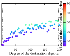
We tested Algorithms 2 and 3 for various small primes, using precomputed Conway polynomials available in Nemo. We do not see major differences between different primes. In Figure 1 we report timings obtained for the case , on an Intel Core i7-7500U CPU clocked at 2.70GHz, using Nemo 0.11.1 running on Julia 1.1.0, and Nemo’s current version of Flint. The plot on the left shows timings for Algorithm 2, for degrees growing from to , for every coprime to and such that the -th Conway polynomial is available in Nemo; the color scale shows the level of the associated algebra . The bottleneck of this algorithm appears to be the -th root extraction routine.
The plot on the right shows timings for Algorithm 3, measured by computing the standard embedding of in . As expected, computing the embeddings takes negligible time in comparison to the decoration of the finite fields. We also tested embedding fields larger than , and noticed that the running time mostly depends on the size of the larger field.

7. Conclusion and future work
We presented a new family of standard compatible polynomials for defining finite fields. Its construction being dependent on the availability of Conway polynomials, it has, at the present moment, very little practical impact; its existence is nevertheless remarkable in itself.
It is even evident that computing our standard polynomials is essentially equivalent to computing Conway polynomials; indeed from one can immediately deduce , and by taking an -th root (doable in polynomial time in ), deduce and the associated Conway polynomial. Hence, an efficient algorithm for computing our polynomials (for arbitrary degrees) would imply an efficient algorithm to compute Conway polynomials, which would be unexpected.
However, our proposed implementation is not the only possible way to exploit our definitions. It would be interesting, indeed, to find some middle ground between the flexibility of the Bosma–Steel–Cannon framework and the rigidity of Conway polynomials, for example by lazily enforcing the conditions required to have a standard solution of (H90), while incrementally constructing the lattice of roots of unity.
Another line of work would be to give a complete implementation of a lattice of finite fields, not limited to extensions of degree coprime to . We leave these questions for future work.
Acknowledgements.
We would like to thank the anonymous reviewers for their useful comments. We thank Éric Schost for fruitful discussions and for helping bootstrap this work during a visit by two of the authors to the University of Waterloo. We acknowledge financial support from the French ANR-15-CE39-0013 project Manta, the OpenDreamKit Horizon 2020 European Research Infrastructures project (#676541), and from the French Domaine d’Intérêt Majeur Math’Innov.References
- (1)
- Allombert (2002) Bill Allombert. 2002. Explicit Computation of Isomorphisms between Finite Fields. Finite Fields and Their Applications 8, 3 (2002), 332 – 342.
- Bosma et al. (1997a) Wieb Bosma, John Cannon, and Catherine Playoust. 1997a. The MAGMA algebra system I: the user language. Journal of Symbolic Computation 24, 3-4 (1997), 235–265. https://doi.org/10.1006/jsco.1996.0125
- Bosma et al. (1997b) Wieb Bosma, John Cannon, and Allan Steel. 1997b. Lattices of compatibly embedded finite fields. Journal of Symbolic Computation 24, 3-4 (1997), 351–369. https://doi.org/10.1006/jsco.1997.0138
- Bostan et al. (2006) Alin Bostan, Philippe Flajolet, Bruno Salvy, and Éric Schost. 2006. Fast computation of special resultants. Journal of Symbolic Computation 41, 1 (2006), 1–29.
- Bostan et al. (2003) Alin Bostan, Grégoire Lecerf, and Éric Schost. 2003. Tellegen’s principle into practice. In ISSAC’03. ACM, 37–44. https://doi.org/10.1145/860854.860870
- Brent and Kung (1978) Richard P. Brent and H.-T. Kung. 1978. Fast Algorithms for Manipulating Formal Power Series. J. ACM 25, 4 (1978), 581–595. https://doi.org/10.1145/322092.322099
- Brieulle et al. (2017) Ludovic Brieulle, Luca De Feo, Javad Doliskani, Jean-Pierre Flori, and Éric Schost. 2017. Computing isomorphisms and embeddings of finite fields (extended version). arXiv preprint arXiv:1705.01221 (2017). https://arxiv.org/abs/1705.01221
- Brieulle et al. (2019) Ludovic Brieulle, Luca De Feo, Javad Doliskani, Jean-Pierre Flori, and Éric Schost. 2019. Computing isomorphisms and embeddings of finite fields. Math. Comp. 88 (2019), 1391–1426. https://doi.org/10.1090/mcom/3363
- Bürgisser et al. (1997) P. Bürgisser, M. Clausen, and M. A. Shokrollahi. 1997. Algebraic Complexity Theory. Springer.
- Couveignes and Lercier (2013) Jean-Marc Couveignes and Reynald Lercier. 2013. Fast construction of irreducible polynomials over finite fields. Israel Journal of Mathematics 194, 1 (01 Mar 2013), 77–105. https://doi.org/10.1007/s11856-012-0070-8
- De Feo et al. (2013) Luca De Feo, Javad Doliskani, and Éric Schost. 2013. Fast algorithms for -adic towers over finite fields. In ISSAC’13. ACM, 165–172.
- De Feo et al. (2014) Luca De Feo, Javad Doliskani, and Éric Schost. 2014. Fast Arithmetic for the Algebraic Closure of Finite Fields. In ISSAC ’14. ACM, 122–129. https://doi.org/10.1145/2608628.2608672
- De Feo and Schost (2012) Luca De Feo and Éric Schost. 2012. Fast arithmetics in Artin-Schreier towers over finite fields. Journal of Symbolic Computation 47, 7 (2012), 771–792. https://doi.org/10.1016/j.jsc.2011.12.008
- Doliskani and Schost (2015) Javad Doliskani and Éric Schost. 2015. Computing in degree -extensions of finite fields of odd characteristic. Designs, Codes and Cryptography 74, 3 (01 Mar 2015), 559–569. https://doi.org/10.1007/s10623-013-9875-7
- Fieker et al. (2017) Claus Fieker, William Hart, Tommy Hofmann, and Fredrik Johansson. 2017. Nemo/Hecke: Computer Algebra and Number Theory Packages for the Julia Programming Language. In ISSAC ’17. ACM, 157–164. https://doi.org/10.1145/3087604.3087611
- Hart et al. (2013) William Hart, Fredrik Johansson, and Sebastian Pancratz. 2013. FLINT: Fast Library for Number Theory. http://flintlib.org Version 2.4.0.
- Heath and Loehr (1999) Lenwood S. Heath and Nicholas A. Loehr. 1999. New algorithms for generating Conway polynomials over finite fields. In SODA ’99. SIAM, 429–437.
- Kedlaya and Umans (2011) Kiran S. Kedlaya and Christopher Umans. 2011. Fast Polynomial Factorization and Modular Composition. SIAM J. Comput. 40, 6 (2011), 1767–1802. https://doi.org/10.1137/08073408X
- Lenstra (1991) Hendrik W. Lenstra. 1991. Finding isomorphisms between finite fields. Math. Comp. 56, 193 (1991), 329–347.
- Lenstra Jr. and de Smit (2013) Hendrick W. Lenstra Jr. and Bart de Smit. 2013. Standard models for finite fields. Chapman and Hall/CRC, Chapter 11.7 in Handbook of Finite Fields, 401–404. https://doi.org/10.1201/b15006
- Narayanan (2018) Anand Kumar Narayanan. 2018. Fast Computation of Isomorphisms Between Finite Fields Using Elliptic Curves. In WAIFI 2018 (LNCS), Vol. 11321. Springer.
- Nickel (1988) Werner Nickel. 1988. Endliche Körper in dem gruppentheoretischen Programmsystem GAP. (1988). https://www2.mathematik.tu-darmstadt.de/˜nickel/
- Roe et al. (2013) David Roe, Jean-Pierre Flori, and Peter Bruin. 2013. Implement pseudo-Conway polynomials. Trac ticket #14958. (Oct. 2013). https://trac.sagemath.org/ticket/14958
- Shoup (1994) Victor Shoup. 1994. Fast construction of irreducible polynomials over finite fields. Journal of Symbolic Computation 17, 5 (1994), 371–391. https://doi.org/10.1006/jsco.1994.1025
- Shoup (1999) Victor Shoup. 1999. Efficient computation of minimal polynomials in algebraic extensions of finite fields. In ISSAC’99. ACM, 53–58. https://doi.org/10.1145/309831.309859
- The GAP Group (2018) The GAP Group 2018. GAP – Groups, Algorithms, and Programming, Version 4.9.2. The GAP Group. https://www.gap-system.org
- The Sage Developers (2019) The Sage Developers 2019. SageMath, the Sage Mathematics Software System (Version 8.7). The Sage Developers. https://www.sagemath.org
- von zur Gathen and Gerhard (1999) Joachim von zur Gathen and Jurgen Gerhard. 1999. Modern Computer Algebra. Cambridge University Press, New York, NY, USA.