Lie symmetries and similarity solutions for rotating shallow water
Abstract
We study a nonlinear system of partial differential equations which describe rotating shallow water with an arbitrary constant polytropic index for the fluid. In our analysis we apply the theory of symmetries for differential equations and we determine that the system of our study is invariant under a five dimensional Lie algebra. The admitted Lie symmetries form the Lie algebra for and for . The application of the Lie symmetries is performed with the derivation of the corresponding zero-order Lie invariants which applied to reduce the system of partial differential equations into integrable systems of ordinary differential equations. For all the possible reductions the algebraic or closed-form solutions are presented. Travel-wave and scaling solutions are also determined.
Keywords: Lie symmetries; invariants; shallow water; similarity solutions
1 Introduction
Lie symmetries is an essential tool for the study of nonlinear differential equations. The main characteristic of the Lie symmetry analysis is that invariant surfaces, in the space where the parameters of the nonlinear differential equation evolve, are determined which can be used to performed an extended analysis of the nonlinear differential equation [1, 2, 3, 4, 5, 6, 7], construct conservation laws [8, 9, 10] and when it is feasible to determine solutions of the differential equation [11, 12, 13, 14]. In applied mathematics Lie symmetries cover a wide range of applications from physics, biology, financial mathematics and many others for instance see [15, 16, 17, 18, 19, 20, 21, 22, 23, 24, 25, 26, 27, 28] and references therein.
In this work, we interest on the application of Lie’s theory on an system of partial differential equations (PDEs) describe one-dimensional rotating shallow water phenomena. The system of our consideration expressed in Lagrangian coordinates is [29]
| (1) | |||||
| (2) | |||||
| (3) |
where denotes the height of the fluid surface, denotes the velocity component in the -direction and is the other horizontal velocity component that is in the direction orhtogonal to the direction [29]. Parameter is the polytropic parameter of the fluid, where in this work is assumed to be The system (1)-(3) is important for the study of atmospheric phenomena like geostrophic adjustment and zonal jets, for more details of the physical properties of the above system we refer the reader in [30, 31, 32] and references therein.
The application of Lie symmetries in shallow-water theory is not new. Indeed, there are various studies in the literature [33, 34, 35, 36, 37, 38] which has been provide important results with special physical interest. Recently, a detailed study of the nonlocal symmetries for a variable coefficient shallow water equation performed in [39]. However, the majority of these studies are for the case where the fluid has a specific polytropic exponent , or the shallow water equations describe non-rotating phenomena. The plan of the paper is as follows.
In Section 2 we present the basic properties and definitions of Lie symmetry analysis which is the main mathematical tool for our analysis. The main results of this work are presented in Section 3. More specifically, we reduce the system (1)-(3) into two equations for the variables and . We derive that the latter system of two PDEs admits five Lie point symmetries and we study all the possible reductions in ordinary differential equations (ODEs) with the use of zero-order Lie invariants. We find that the reduce systems can be solve explicitly and we derive the algebraic solution or closed-form solutions for every possible reduction and every value of the parameter . The latter result is important because it shows how powerful is the method of Lie symmetry analysis for the study of shallow-water phenomena to prove the existence of solutions for the model of our study. Emphasis is given on the travel-wave and scaling solutions. Finally our discussion and conclusions are presented in Section 4.
2 Preliminaries
In this Section we briefly discuss the basic definitions and main steps for the determination of Lie point symmetries for differential equations.
Consider a system of PDEs
| (4) |
where denotes the dependent variables, are the indepedent variables and .
We assume the one-parameter point transformation (1PPT) in the space of the independent and dependent variables
| (5) | |||||
| (6) |
in which is an infinitesimal parameter, the differential equation (4) remain invariant if and only if
| (7) |
or equivalently [12]
| (8) |
The latter conditions is expressed
| (9) |
where denotes the Lie derivative with respect the vector field which is the th-extension of generator of the infinitesimal transformation (5), (6) in the jet space
| (10) |
with generator
| (11) |
and
| (12) |
When condition (9) is satisfied for a specific 1PPT, the vector field is called a Lie point symmetry for the system of PDEs (4). For an unknown 1PPT, in order to specify the generators which are Lie point symmetries for a given differential equation, from the symmetry condition (9) we specify a system of PDEs with dependent variables the components of the generator . The solution of the latter system provides the generic symmetry vector and the number of independent solutions give the number of indepedent vector field and the dimension of the admitted Lie algebra.
3 Lie symmetry analysis
We write the system (1)-(3) as two second-order PDEs
| (13) | |||||
| (14) |
while the application of Lie’s theory provides a five dimensional Lie algebra consists by the following vector fields
In table 1 the commutators of the Lie symmetries are presented. Consequently, from table 1 we can refer that the admitted Lie algebra is the in the Morozov-Mubarakzyanov Classification Scheme [40, 41, 42, 43]. However, in the limit where , the admitted Lie algebra is the .
In order to continue with the application of the Lie point symmetries it is important to determine the one-dimensional optimal system and invariants [44]. In order to do that the adjoint representations should be calculated. By definition, for every basis of the Lie symmetries , the adjoint representation is given by the following expression
| (15) |
For the admitted Lie point symmetries of the system (13), (14) the adjoint representation are given in 2. In order to find the optimal system we consider the generic symmetry vector
| (16) |
and we find the equivalent vectors by considering the adjoint representation. At this point it is important to mention that the adjoint action admits two invariant functions, the and [45]. The invariants can be used to simplify the calculations on the derivation of the optimal system. Indeed we have to consider the cases and .
Case 1: For , we have that
becomes
for specific values of the parameters and .
Case 2: For , there are three subcases, (a) , ; (b) , and (c) .
Case 2a: For and , and following the steps as before we find the optimal system where . In the limit , the generic optimal system is .
Case 2b: For and the optimal system is derived
which for specific values of and is simplified as
Parameter is not an invariant hence, it can be zero too. Hence, the two optimal systems are and .
Case 2c: For , we calculate the generic optimal systems .
Hence, the one-dimensional optimal systems for
and for
There is a difference in the number of one-dimensional optimal systems which depends on the parameter , that is expected because the structure of the Lie algebra changes.
We proceed our analysis by applying the Lie symmetries to reduce the system of PDEs into a system of ODEs and solve the resulting ODEs by applying the method of Lie symmetries.
3.1 Static solution
3.2 Point solution
The application of the symmetry vector provides with the time-dependent solution in a specific point, i.e. and . The resulting system provides and the second-order ODE
| (18) |
The later equation is nothing else than the oscillator which admits eight Lie point symmetries and it is maximally symmetric. The Lie symmetries and are inherit symmetries, while the rest five Lie point symmetries are Type II symmetries. The exact solution of equation (18) is
| (19) |
3.3 Travel-wave solution
The linear combination of provides travel-wave solutions where parameter describes the the wave speed. The reduced system is
| (20) | |||||
| (21) |
in which the new independent parameter is defined as .
The latter equation admits only one Lie point symmetry for , the autonomous symmetry Recall that for equation (23) becomes a maximally symmetric equation but such value for parameter is not physical accepted.
Application of the differential invariants of the autonomous symmetry vector in (23) lead to the nonlinear first-order ODE
| (24) |
with solution
| (25) |
where the new variables are defined as and .
In the simplest case where the integration constant vanishes, and , the generic solution is given in terms of the Lambert function
| (26) |
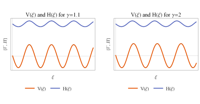
In Fig. 1 we present a numerical simulation of the and as they provided by the differential equation (23). The plots which are presented are for and . From the figure we observe a travelling-wave solution for , and for the variable .
3.4 Scaling solution
The Lie invariants of the scaling symmetry vector are
| (27) |
Hence, the reduced system consists by two second-order ODEs
| (28) | |||||
| (29) |
From (28) and for we find
| (30) |
and replacing in (29) we end up with one second-order ODE with dependent variable the , i.e.,
| (31) |
where we have replaced in order to simplify the form of the differential equation.
For arbitrary parameter , equation (31) admits only the autonomous symmetry vector . In the special case where and equation (31) is invariant under the Lie algebra and reduce to the Ermakov-Pinney equation [46, 47]. We proceed with the application of the autonomous vector field.
The Lie invariants of the autonomous symmetry are and , hence, equation (31) reduces to the first-order ODE
| (32) |
with solution
| (33) |
For , the Lie invariants of the scaling symmetry are , where the reduced system gives, , i.e. and .
3.5 Reduction with the vector fields
The existence of the two symmetry vectors , or of the more general symmetry , indicates that the system of our consideration (13)-(14) is invariant under the point transformation
| (34) |
Consequently, by taking any linear combination of the other symmetries with the vector field we determine the same reduced equations, where the invariants have been transformed according to the rule (34), except to the case of point reduction, i.e. and scaling solution for , which are the two cases we present in the following lines.
3.5.1 Reduction with
By considering the Lie invariants in (13)-(14) of the symmetry vector we find and where
| (35) | |||||
| (36) |
Therefore, the main difference with the point reduction solution is that the height is not a constant anymore, and it is given by
| (37) |
while now
| (38) |
It is important here to mention that in order to avoid singular behaviour in finite time, then the integration constants while . The latter solution provide a linear spread of the velocities in the space.
3.5.2 Reduction with for
The case of scaling solutions with when we consider the symmetry vector in the reduction is totally different from the case before. Indeed, the Lie invariants are
| (39) |
where and satisfy the reduced equations
| (40) | |||||
| (41) |
From (40) it follows
| (42) |
where by replacing in (41) gives a maximally symmetric second-order ODE with generic solution
| (43) | |||||
while the conditions follows in order to avoid singularities at finite time.
In contrary with the previous reduction where the evolution of the speeds in the space is linear, in this case, the speed evolve with a logarithmic expansion which provide an initial singularity at .
3.6 Reduction with the vector fields
For the vector field , where is nonzero constant the Lie invariants are derived to be
| (44) |
from where by replacing in (13)-(14) we find the reduced system
| (45) |
| (46) |
An exact solution for the later system can be calculated by assuming a power-law behaviour for the functions and . Indeed we find the special solution
| (47) |
with constraint equation
| (48) |
4 Conclusions
In this work we studied a system of nonlinear PDEs which describe rotating shallow-water with the method of Lie symmetries. More specifically, we determine the Lie symmetries for the system (13)-(14) and we found that the system of PDEs is invariant under a five dimensional Lie algebra. The admitted Lie symmetries form the Lie algebra in the Morozov-Mubarakzyanov Classification Scheme for the parameter or the Lie algebra when . That difference in the admitted Lie algebra between the two cases and are observable in the application of Lie symmetries and more specifically in the reduction process.
Indeed for any symmetry vector we considered the application of the zero-order Lie invariants and we rewrote the system of PDEs into a system ODEs which we were able to solve them explicitly in all cases by using the Lie symmetry analysis. Another important feature of the Lie symmetries is that we can transform solutions into solutions after the application of the invariant 1PPT.
It is important to mention that someone could started the present analysis by studying the original three-dimensional first-order differential equations (1)-(3). Either in that approach the results of the analysis will not change, except from that the point transformation is defined in the space of variables . In our analysis we consider to study the point transformations defined in the space of variable . Now by extending the symmetry vectors obtained in the space in the (partial-) extension space , the symmetry vectors become
where by replacing . are the Lie point symmetries of the original system (1)-(3).
We conclude that with the application of Lie symmetries we were able to prove the existence of solutions for the rotating shallow wave system (13)-(14). Another important observation is that the reduced differential equations were reduced into well-known first-order ODEs. Finally, we proved the existence of travel-wave and scaling solutions.
Acknowledgements
The author acknowledges the partial financial support of FONDECYT grant no. 3160121 and thanks the University of Athens for the hospitality provided.
Appendix A Lie symmetry analysis in the Euler coordinates
The symmetry analysis provide the same results in the Euler coordinates. The applications of the symmetry condition (9) gives the symmetry vector fields
The latter symmetry vectors form the same Lie algebras with that of system (1)-(3). Because they are in a different representation with the vector fields , the invariant functions are different. Vector fields and provide static and stationary solutions while the linear combination gives the similarity solution which describe traveling waves. For the vector field provide the scaling invariants
| (56) |
where functions and satisfy the following system of first-order ODEs
| (57) | |||||
| (58) | |||||
| (59) |
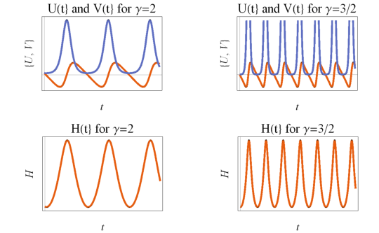
The latter system can be easily integrated, however its general solution it is not given by a closed-form expression. Numerical simulations of the latter system are presented in Fig. 2 for two values of the parameter More specifically for and . From the figures we observe periodic behaviour for the dynamical parameters of the dynamical system.
Finally, the symmetry vector provide the generic solution
| (60) |
where
| (61) |
References
- [1] L. V. Ovsiannikov, Group analysis of differential equations, Academic Press, New York, (1982)
- [2] B.K. Harrison, Sigma 1, 001 (2005)
- [3] V.A. Baikov, A.V. Gladkov and R.J. Wiltshire, J. Phys. A: Math. Gen. 31, 7483 (1998)
- [4] T.G. Mkhize, K. Govinder, S. Moyo and S.V. Meleshko, Appl. Math. Comput. 301, 25 (2017)
- [5] A. Paliathanasis and P.G.L. Leach, Int. J. Geom. Meth. Mod. Phys. 13, 1630009 (2016)
- [6] M.C. Nucci and P.G.L. Leach, J. Math. Anal. Appl. 406, 219 (2013)
- [7] M.C. Nucci, J. Nonl. Math. Phys. 20, 451 (2013)
- [8] E. Noether, Nachr. d. König. Gesellsch. d. Wiss. zu Göttingen, Math-phys. Klasse, 235, (1918) (translated in English by M.A. Tavel [physics/0503066])
- [9] N.H. Ibragimov, J. Math. Anal. Appl. 333, 311 (2007)
- [10] W. Sarlet and F. Cantrijin, SIAM Review, 23, 467 (1981)
- [11] P.J. Olver, Applications of Lie Groups to Differential Equations, Springer-Verlag, New York, (1993)
- [12] G.W. Bluman and S. Kumei, Symmetries and Differential Equations, Springer-Verlag, New York, (1989)
- [13] N.H. Ibragimov, CRC Handbook of Lie Group Analysis of Differential Equations, Volume I: Symmetries, Exact Solutions, and Conservation Laws, CRS Press LLC, Florida (2000)
- [14] S.V. Meleshko, Methods for Constructing Exact Solutions of Partial Differential Equations, Springer Science, New York (2005)
- [15] S.V. Meleshko and V.P. Shapeev, J. Nonl. Math. Phys. 18, 195 (2011)
- [16] G.M. Webb and G.P. Zank, J. Math. Phys. A: Math. Theor. 40, 545 (2007)
- [17] M.C. Nucci and G. Sanchini, Symmetry 7, 1613 (2015)
- [18] A. Paliathanasis, K. Krishnakumar, K.M. Tamizhmani and P.G.L. Leach, Mathematics 4, 28 (2016)
- [19] X. Xin, Appl. Math. Lett. 55, 63 (2016)
- [20] X. Xin, Acta Phys. Sin. 65, 240202 (2016)
- [21] N. Kallinikos and E. Meletlidou, J. Phys. A: Math. Theor. 46, 305202 (2013)
- [22] S. Jamal and A. Paliathanasis, J. Geom. Phys. 117, 50 (2017)
- [23] G.M. Webb, J. Phys A: Math. Gen. 23, 3885 (1990)
- [24] P.G.L. Leach, J. Math. Anal. Appl. 348, 487 (2008)
- [25] M. Tsamparlis and A. Paliathanasis, J. Phys. A: Math. Theor. 44, 175202 (2011)
- [26] M. Tsamparlis and A. Paliathanasis, Symmetry (MDPI) 10, 233 (2018)
- [27] X. Xin, Commun. Theor. Phys. 66, 479 (2016)
- [28] X. Xin, H. Liu, L. Zhang and Z. Wang, Appl. Math. Lett. 88, 132 (2019)
- [29] B. Cheng, P. Qu and C. Xe, SIAM J. Math. Anal. 50, 2486 (2018)
- [30] B. Galperin, H. Nakano, H.-P. Huang, and S. Sukoriansky, Geoph. Res. Let. 31, L13303 (2004)
- [31] V. Zeitlin, S. B. Medvedev, and R. Plougonven, J. Fluid. Mech. 481, 269 (2003)
- [32] D.A. Randall, Monthly Weather Review 122, 1371 (1994)
- [33] M. Senthilvelan and M. Lakshmanan, Int. J. Nonl. Mech. 31, 339 (1996)
- [34] S. Szatmari and A. Bihlo, Comm. Nonl. Sci. Num. Sim. 19, 530 (2014)
- [35] A.A. Chesnokov, J. Appl. Mech. Techn. Phys. 49, 737 (2008)
- [36] J.-G. Liu, Z.-F. Zeng, Y. He and G.-P. Ai, Int. J. Nonl. Sci. Num. Sim. 16, 114 (2013)
- [37] A.A. Chesnokov, Eur. J. Appl. Math. 20, 461 (2009)
- [38] M. Pandey, Int. J. Nonl. Sci. Num. Sim. 16, 93 (2015)
- [39] X. Xin, L. Zhang, Y. Xia and H. Liu, Appl. Math. Lett. 94, 112 (2019)
- [40] Morozov VV (1958), Izvestia Vysshikh Uchebn Zavendeniĭ Matematika, 5 161-171
- [41] Mubarakzyanov GM (1963), Izvestia Vysshikh Uchebn Zavendeniĭ Matematika, 32 114-123
- [42] Mubarakzyanov GM (1963), Izvestia Vysshikh Uchebn Zavendeniĭ Matematika, 34 99-106
- [43] Mubarakzyanov GM (1963), Izvestia Vysshikh Uchebn Zavendeniĭ Matematika, 35 104-116
- [44] P.J. Olver, Applications of Lie Groups to Differential Equations, second edition, Springer-Verlag, New York (1993)
- [45] X. Hu, Y. Li and Y. Chen, J. Math. Phys. 56, 053504 (2015)
- [46] V. Ermakov, Universita Izvestia Kiev Series III 9 1-25 (1880) (The English version, translated by AO Harin, can be found in Applicable analysis and Discrete Mathematics)
- [47] E. Pinney, Proceedings of the American Mathematical Society 1, 681 (1950)