Decentralized Deep Reinforcement Learning for Delay-Power Tradeoff in Vehicular CommunicationsX. Chen and H. Vuojala are with the VTT Technical Research Centre of Finland, Finland (email: {xianfu.chen, heli.vuojala}@vtt.fi). C. Wu is with the Graduate School of Informatics and Engineering, University of Electro-Communications, Japan (email: clmg@is.uec.ac.jp). H. Zhang is with the College of Information Science and Electronic Engineering, Zhejiang University, China (e-mail: honggangzhang@zju.edu.cn). Y. Zhang is with the Department of Informatics, University of Oslo, Norway (e-mail: yanzhang@ieee.org). M. Bennis is with the Centre for Wireless Communications, University of Oulu, Finland (email: mehdi.bennis@oulu.fi).
Abstract
This paper targets at the problem of radio resource management for expected long-term delay-power tradeoff in vehicular communications. At each decision epoch, the road side unit observes the global network state, allocates channels and schedules data packets for all vehicle user equipment-pairs (VUE-pairs). The decision-making procedure is modelled as a discrete-time Markov decision process (MDP). The technical challenges in solving an optimal control policy originate from highly spatial mobility of vehicles and temporal variations in data traffic. To simplify the decision-making process, we first decompose the MDP into a series of per-VUE-pair MDPs. We then propose an online long short-term memory based deep reinforcement learning algorithm to break the curse of high dimensionality in state space faced by each per-VUE-pair MDP. With the proposed algorithm, the optimal channel allocation and packet scheduling decision at each epoch can be made in a decentralized way in accordance with the partial observations of the global network state at the VUE-pairs. Numerical simulations validate the theoretical analysis and show the effectiveness of the proposed online learning algorithm.
I Introduction
The vehicle-to-vehicle (V2V) communication technologies have been gaining increasing popularity for the feasibility of enabling emerging vehicle-related services [1, 2, 3]. However, this ad hoc type of vehicular communications requires intense coordinations among the vehicles in close proximity [4]. Without the support of an infrastructure, the high vehicle mobility makes the design of efficient radio resource management (RRM) techniques extremely challenging [5]. There are a large body of literatures on RRM in V2V communications. In [6], Sun et al. proposed a separate resource block and power allocation algorithm for the RRM in device-to-device based V2V communications. In [7], Yao et al. derived a loss differentiation rate adaptation scheme to meet the stringent delay and reliability requirements for V2V safety communications. In [8], Egea-Lopez et al. designed a fair adaptive beaconing rate algorithm for the problem of beaconing rate control in inter-vehicular communications. Most of these efforts have not taken into account the network dynamics, such as the temporal and spatial variations in transmission quality as well as data traffic, and hence fail to optimize the expected long-term RRM performance.
A Markov decision process (MDP) has been successfully applied to model RRM in vehicular communications with time-varying nature. In [9], Liu and Bennis formulated a latency and reliability [10] constrained transmit power minimization problem, for which the Lyapunov stochastic optimization was leveraged to handle the network dynamics. The problem with the Lyapunov stochastic optimization is that only an approximately optimal solution can be constructed. In [11], Chen et al. studied the non-cooperative RRM in vehicular communications from an oblivious game-theoretic perspective and put forward an online algorithm based on reinforcement learning to approach the optimal solution. Consider a more practical scenario, where the channel qualities are affected by the vehicle mobility, the explosion in the state space makes the technique developed in our priori work [11] infeasible.
In this paper, we investigate a Manhattan grid V2V network, where the data traffic changes across the time horizon and the channel quality state depends on the locations of vehicle user equipment (VUE)-transmitter (vTx) and VUE-receiver (vRx) of a VUE-pair. The primary goal of this paper is to design an optimal RRM algorithm for each VUE-pair to strike a tradeoff between the queuing delay and the transmit power consumption over the long run. We formulate the RRM problem as a MDP and resort to a deep neural network based function approximator to deal with the curse of state space explosion [12]. In [13], Ye and Li devised a decentralized RRM mechanism based on deep reinforcement learning (DRL) for V2V communication systems. However, the mechanism does not account for the vehicle mobility, which helps facilitate frequency resource sharing among different groups of VUE-pairs. As the major contribution from this paper, we propose an online decentralized learning algorithm by exploring the recent advances in both long short-term memory (LSTM) [14] and DRL [15], with which each VUE-pair with partially local network state observations is hence able to realize a significant performance improvement.
II System Model
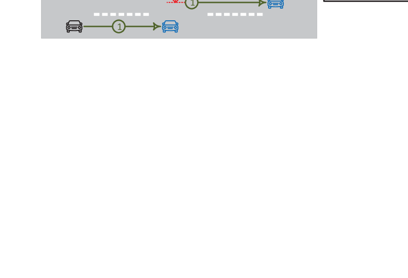
As in Fig. 1, we consider a Manhattan grid V2V communication scenario. A set 11 1 For a well defined road segment, the VUE density tends to be steady [16]. of VUE-pairs share a set of orthogonal channels within the coverage of a road side unit (RSU), where represents a two-dimensional Euclidean space. The time horizon is discretized into decision epochs, each of which is of duration and is indexed by an integer . Each vTx always follows the corresponding vRx with a fixed distance of and the vRx moves in according to a Manhattan mobility model [11]. Denote by and , respectively, the Euclidean coordinates of the vTx and the vRx of a VUE-pair during each epoch . Depending on whether the vTx and the vRx are in the same lane or in perpendicular lanes, the channel model during each decision epoch belongs to: 1) line-of-sight (LOS) – both the vTx and the vRx are in the same lane; 2) weak-line-of-sight (WLOS) – the vTx and the vRx are in perpendicular lanes and at least one of them is near the intersection within a distance of ; and otherwise, 3) none-line-of-sight (NLOS). More specifically, the channel quality state experienced by VUE-pair over channel during epoch includes a fast fading component of a Rayleigh distribution with a unit scale parameter and a path loss that applies the model in (II) for urban areas using 5.9 GHz carrier frequency [9],
where is the path loss coefficient while and are the path loss exponents with .
In order to mitigate the interference during wireless transmissions and maximize the channel utilization, the RSU clusters22 2 Considering the vehicle mobility, clustering is done every epochs [9]. the VUE-pairs into a set of disjoint groups based on their geographical locations, where . The RSU allocates channels to the groups, while in each group, we assume that a VUE-pair can be assigned at most one channel and a channel can be assigned to at most one VUE-pair. Let denote the channel allocation for a VUE-pair during decision epoch , where is the set of VUE-pairs in a group and
Thus we have
| (7) | ||||
| (8) |
At the vTx of each VUE-pair , a data queue is maintained to buffer the arriving packets. Let be the random new packet arrivals at epoch with average arrival rate . The queue evolution for VUE-pair can be expressed as
| (9) |
where and are, respectively, the queue length and the number of packets to depart during decision epoch , while is an indicator function that equals if the condition is satisfied and otherwise. In this paper, we assume a large enough buffer size to neglect the probability of packet drops. The required transmit power for delivering packets can be computed as
| (10) |
where is the received interference due to inter-group channel reuse, is the frequency bandwidth of the channels, is the power spectral density of additive background noise, and is the constant size of a data packet.
III Problem Description
This section formulates the problem of RRM in the considered V2V network as a discrete-time MDP with a discounted criterion and discusses the general solution.
III-A MDP Formulation
During each decision epoch , the local state of a VUE-pair can be described by , which includes the information of channel quality , geographical location and queue state . We use to represent the global network state, where denotes all the other VUE-pairs in without the presence of VUE-pair . The RSU aims to design a stationary control policy , where and are, respectively, the channel allocation policy and the packet scheduling policy. Specifically, the RSU observes at the beginning of epoch and accordingly, makes channel allocation and packet scheduling decisions for the VUE-pairs, that is, , where and . From the assumptions on the mobility of a VUE-pair, the packet arrivals and the queue evolution, the randomness lying in is Markovian with the following controlled state transition probability
| (11) |
where denotes the probability of an event.
We need a cost function to tradeoff the queuing delay and the consumed transmit power for each VUE-pair during each decision epoch , which can be chosen as
| (12) |
where , while and are two positive weights. Given a control policy and an initial global network state , we express the expected long-term cost function for VUE-pair as
| (13) |
where is the discount factor. As a result, the delay-power tradeoff problem, which the RSU aims to solve, can be formally formulated as a MDP, namely, ,
| (14) | ||||
where is the immediate cost accumulated across all the VUE-pairs in the network at a decision epoch . is also named as the state value function in state under a policy .
III-B Optimal Solution
The problem formulated as in (14) is a typical infinite-horizon discrete-time MDP with a discounted criterion. Denote by the optimal control policy, which can be obtained from solving the Bellman’s equation: ,
| (15) | ||||
where is the optimal state value function and is the resulting global network state at a subsequent epoch. The conventional solutions to (15) based on the value or policy iteration [17] require the complete knowledge of network dynamics (III-A), which is challenging in practice. Let us define the right-hand side of (15) by
| (16) |
the -function, where and are the decision makings under with . can then be directly obtained from
| (17) |
By substituting (17) back into (III-B), we have
| (18) |
where and denote the decision makings under with .
Using a state-action-reward-state-action (SARSA) algorithm [18, 17], the RSU tries to learn in a recursive way with observations of the global network state , the decision making , the realized cost at a current decision epoch and the resulting global network state , the decision making at the next epoch . The updating rule is given by
| (19) | ||||
where is the learning rate. It has been proven that if 1) the network state transition probability under the optimal stationary control policy is stationary, 2) is infinite and is finite, and 3) all state-action pairs are visited infinitely often (which can be satisfied by a -greedy strategy [17]), the SARSA learning process converges and finds [19]. However, two challenges remain as follows:
- 1.
from the channel model applied in this work, the global network state space is semi-continuous; and
- 2.
the number of decision makings at the RSU grows exponentially as increases, where is the maximum number of packet departures at a vTx, i.e., , and .
IV A Deep Reinforcement Learning Approach
We shall address in this section the technical challenges in solving an optimal control policy and derive a deep reinforcement learning algorithm.
IV-A Linear -function Decomposition
The centralized decisions made by the RSU are performed by the VUE-pairs in a decentralized way. We hence propose to linearly decompose the -function, that is,
| (20) |
where is the per-VUE-pair -function for each VUE-pair that satisfies
| (21) | ||||
where the optimal decision making from a VUE-pair across the time horizon should reflect the optimal control policy implemented by the RSU. In other words, in (21) under the network state follows , i.e.,
| (22) |
which minimizes the sum of per-VUE-pair -function values from all VUE-pairs in the network. Two key advantages of the decomposition approach in (20) are highlighted.
- 1.
Simplified decision makings: The linear decomposition motivates the RSU to let the VUE-pairs submit the local per-VUE-pair -functions of the channel allocation and packet scheduling decisions with the global network state observations, based on which the RSU allocates channels and the VUE-pairs then schedule packet transmissions. This reduces centralized decision makings at the RSU to decentralized decisions for all VUE-pairs.
- 2.
IV-B Learning the Optimal Control Policy
In spite of the advantages brought by the linear decomposition approach as in (20), a new challenge, however, arises. That is, each VUE-pair can only obtain a partial observation of the global network state at each decision epoch . In this work, we assume that when VUE-pair was in a group (i.e., ) during the previous decision epoch , includes the group index and the number of VUE-pairs as well as the channel utilization state in group , where equals if channel is utilized in group at epoch and otherwise, . Note that is restricted to local group information since the decision makings across different groups are independent.
With the local observation at a current decision epoch, we abstract the per-VUE-pair -function (21) of each VUE-pair as [20]
| (23) |
The semi-continuity in and the high dimensionality in make it infeasible for the conventional SARSA algorithm (19) to learn the per-VUE-pair -function , . Moreover, from the assumptions made in this paper and the definition of a cost function (12), there exists homogeneity in the VUE-pair behaviours. Inspired by the success of modelling the -function with a deep neural network (DNN) [12], we adopt a common double deep -network (DQN) to approximate [15, 21]. On the other hand, the accuracy of (23) from the observations can be, in general, arbitrarily bad. As in [22], we propose to add a LSTM layer [14] to the DQN and obtain a hybrid DNN to learn a better control policy in a partially observable V2V network. Specifically, let , , where denotes a set of most recent local observations up to a current decision epoch (which will be specified later in this subsection) and is taken as an input to the LSTM layer for a more accurate prediction of , while denotes a vector of parameters associated with the hybrid DNN. Our proposed novel LSTM based deep reinforcement learning (LSTM-DRL) algorithm for long-term delay-power tradeoff in the considered V2V network is illustrated in Fig. 2, during which instead of finding the per-VUE-pair -function, the parameters of the hybrid DNN can be trained centrally at the RSU.

For online training of the LSTM-DRL algorithm, at each decision epoch , the RSU updates the replay memory with the most recent experiences with each experience () being given by
| (24) |
Meanwhile, an observation pool , the information of which is collected from all VUE-pairs, is kept to predict the global network state at epoch for control policy evaluation, where . To train the hybrid DNN parameters, the RSU first randomly samples a mini-batch of size from , where ,
| (25) |
with . Then the set of parameters at epoch is updated by minimizing the accumulative loss function, which is defined as in (IV-B),
where is the set of parameters of the target hybrid DNN at a certain previous decision epoch before epoch . The gradient is calculated as (IV-B).
We summarize in Algorithm 1 the online training of the proposed LSTM-DRL algorithm.
V Simulation Results
This section evaluates the performance from our proposed studies through numerical simulations based on TensorFlow [23]. We simulate a m2 Manhattan mobility model with nine intersections [9, 11]. In the model, a road consists of two lanes, each of which is in one direction and is of width m. The average vehicle speed is set to be km/h, and the vehicle grouping is performed by means of spectral clustering [11]. We list other parameter values used in simulations in Table I. For performance comparison purpose, the following three baseline algorithms are simulated as well.
- 1.
Channel-Aware: At each decision epoch, the RSU allocates the channels to VUE-pairs in each group based on the channel quality states.
- 2.
Queue-Aware: Different from the Channel-Aware algorithm, the RSU allocates at each decision epoch the channels to VUE-pairs in each group according to the queue lengths.
- 3.
Random: Across the decision epochs, the RSU randomly allocates the channels to a set of randomly picked VUE-pairs in each group.
Implementing these baselines, the RSU schedules packets to minimize the immediate cost for each VUE-pair.
| Parameter | Value |
|---|---|
| Replay memory capacity | |
| Mini-batch size | |
| Observation pool size | |
| Path loss exponent , | dB, dB |
| Path loss coefficient | |
| Distance | m |
| Number of VUE-pair group | |
| Clustering interval | epochs |
| Frequency bandwidth | kHz |
| Aggregate interference | W |
| Noise power spectral density | W/Hz |
| Scheduling epoch duration | ms |
| Weights , | , |
| Data packet size | kb |
| Discount factor | |
| Exploration probability |
V-A Convergence Property of the Proposed Algorithm
This simulation examines the convergence property of online training of our LSTM-DRL algorithm. We select VUE-pairs with an average packet arrival rate , and the distance between the VTx and the vRx of each VUE-pair is fixed to be . Fig. 3 plots the loss function defined by (IV-B) over the learning time horizon, which validates that the convergence needs around decision epochs. Since the training is performed centrally at the RSU, each VUE-pair only needs to periodically update the set of parameters of the LSTM-DRL algorithm with a new one from the RSU.


V-B Performance under Various Simulation Settings
We further verify the average cost performance per VUE-pair across the time horizon under different simulation settings. First, we configure a networking environment as: and . In Fig. 4(a), we depict the realized average cost performance versus , which shows the average cost per VUE-pair from all four algorithms increases as the number of VUE-pairs increases. It is obvious that a larger number of VUE-pairs leads to less chance of being allocated one channel. Next, we assume there are VUE-pairs in the network and . By increasing the value of , the average cost performance per VUE-pair is shown in Fig. 4(b) With more packets arriving into the queues, more power is consumed for the packet transmissions in order to maintain the queue stability. Hence all four algorithms exhibit worse performance. Finally, we illustrate in Fig. 4(c) the average cost performance per VUE-pair when the value of varies. As the distance between the vTx and the vRx of a VUE-pair increases, the channel quality drops. This indicates more transmit power for transmitting the same number of packets, which conforms what we see from the curves in Fig. 4(c). Interestingly and importantly, in all above three simulations, our proposed algorithm achieves the best performance, demonstrating the feasibility of a better delay-power tradeoff, compared with the other three baselines.
VI Conclusions
In this paper, we put our emphasis on investigating the RRM for an expected long-term delay-power tradeoff in a V2V communication network. The RSU allocates channels and schedules packet transmissions for all VUE-pairs according to the observations of global network states over the discrete time horizon. This kind of decision-making process straightforwardly falls into the realm of a MDP. The technical challenges in solving an optimal control policy for the MDP motivates us to first decompose the MDP into a series of per-VUE-pair MDPs with much simplified decision makings. To overcome the curse of high dimensionality in state space of a per-VUE-pair MDP, we resort to the DQN technique and propose an online LSTM-DRL algorithm. The LSTM-DRL algorithm enables decentralized channel allocation and packet scheduling decisions with only partially local network state observations from the VUE-pairs but without a priori statistics knowledge of network dynamics. From numerical simulations, significant gains in average cost performance from the proposed learning algorithm can be expected.
References
- [1] S. Kuutti et al., “A survey of the state-of-the-art localization techniques and their potentials for autonomous vehicle applications,” IEEE Internet Things J., vol. 5, no. 2, pp. 829–846, Mar. 2018.
- [2] Y. Dai, D. Xu, S. Maharjan, G. Qiao, and Y. Zhang, “Artificial intelligence empowered edge computing and caching for internet of vehicles,” IEEE Wireless Commun. Mag., accepted, 2019.
- [3] K. Zhang, S. Leng, X. Peng, P. Li, S. Maharjan, and Y. Zhang, “Artificial intelligence inspired transmission scheduling in cognitive vehicular communications and networks,” IEEE Internet Things J., Early Access Article, 2018.
- [4] M. Amadeo, C. Campolo, and A. Molinaro, “Information-centric networking for connected vehicles: A survey and future perspectives,” IEEE Commun. Mag., vol. 54, no. 2, pp. 98–104, Feb. 2016.
- [5] K. Zheng, Q. Zheng, P. Chatzimisios, W. Xiang, and Y. Zhou, “Heterogeneous vehicular networking: A survey on architecture, challenges, and solutions,” IEEE Commun. Surveys Tuts, vol. 17, no. 4, pp. 2377–2396, Q4 2015.
- [6] W. Sun, E. G. Ström, F. Brännström, K. C. Sou, and Y. Sui, “Radio resource management for D2D-based V2V communication,” IEEE Trans. Veh. Technol., vol. 65, no. 8, pp. 6636–6650, Aug. 2016.
- [7] Y. Yao, X. Chen, L. Rao, X. Liu, and X. Zhou, “LORA: Loss differentiation rate adaptation scheme for vehicle-to-vehicle safety communications,” IEEE Trans. Veh. Technol., vol. 66, no. 3, pp. 2499–2512, Mar. 2017.
- [8] E. Egea-Lopez and P. Pavon-Mariño, “Distributed and fair beaconing rate adaptation for congestion control in vehicle network,” IEEE Trans. Mobile Comput., vol. 15, no. 12, pp. 3028–3041, Dec. 2016.
- [9] C.-F. Liu and M. Bennis, “Ultra-reliability and low-latency vehicular transmissions: An extreme value theory approach,” IEEE Commun. Lett., vol. 22, no. 6, pp. 1292–1295, May 2018.
- [10] M. Bennis, M. Debbah, and H. V. Poor, “Ultrareliable and Low-Latency Wireless Communication: Tail, Risk, and Scale,” Proc. of the IEEE, vol. 106, no. 10, pp. 1834–1853, Oct. 2018.
- [11] X. Chen, C. Wu, M. Bennis, Z. Zhao, and Z. Han, “Learning to entangle radio resources in vehicular communications: An oblivious game-theoretic perspective,” IEEE Trans. Veh. Technol., vol. 68, no. 5, pp. 4262–4274, May 2019.
- [12] V. Mnih et al., “Human-level control through deep reinforcement learning,” Nature, vol. 518, no. 7540, pp. 529–533, Feb. 2015.
- [13] H. Ye and G. Y. Li, “Deep reinforcement learning for resource allocation in V2V communications,” in Proc. IEEE ICC, Kansas City, MO, May 2018.
- [14] S. Hochreiter and J. Schmidhuber, “Long short-term memory,” Neural Comput., vol. 9, no. 9, pp. 1735–1780, Nov. 1997.
- [15] H. van Hasselt, A. Guez, and D. Silver, “Deep reinforcement learning with double Q-learning,” in Proc. AAAI, Phoenix, AZ, Feb. 2016.
- [16] Y. Zhuang, J. Pan, V. Viswanathan, and L. Cai, “On the uplink MAC performance of a drive-thru internet,” IEEE Trans. Veh. Technol., vol. 61, no. 4, pp. 1925–1935, May 2012.
- [17] R. S. Sutton and A. G. Barto, Reinforcement Learning: An Introduction. Cambridge, MA: MIT Press, 1998.
- [18] G. A. Rummery and M. Niranjan. Online Q-learning using connectionist systems, Tech. Rep. CUED/F-INFENG/TR 166, Cambridge University Engineering Department, Sep. 1994.
- [19] S. Singh, T. Jaakkola, M. L. Littman, and C. Szepesvári, “Convergence results for single-step on-policy reinforcement-learning algorithms,” Mach. Learn., vol. 38, no. 3, pp. 287–308, Mar. 2000.
- [20] X. Chen et al., “Wireless resource scheduling in virtualized radio access networks using stochastic learning,” IEEE Trans. Mobile Comput., vol. 17, no. 4, pp. 961–974, Apr. 2018.
- [21] Y. Dai, D. Xu, S. Maharjan, Z. Chen, Q. He, and Y. Zhang, “Blockchain and deep reinforcement learning empowered intelligent 5G beyond,” IEEE Netw., accepted, 2019.
- [22] M. Hausknecht and P. Stone, “Deep recurrent Q-learning for partially observable MDPs,” in Proc. AAAI, Austin, TX, Jan. 2015.
- [23] M. Abadi et al., “Tensorflow: A system for large-scale machine learning,” in Proc. OSDI, Savannah, GA, Nov. 2016.