eurm10 \checkfontmsam10
Shear induced migration of microswimmers in pressure-driven channel flow
Abstract
We study the shear induced migration of microswimmers (primarily, active Brownian particles or ABP’s) in plane Poiseuille flow. For wide channels characterized by , the separation between time scales characterizing the swimmer orientation dynamics (of O()) and those that characterize migration across the channel (of O()), allows for use of the method of multiple scales to derive a drift-diffusion equation for the swimmer concentration profile; here, is the swimming speed, is the channel half-width, and is the swimmer rotary diffusivity. The steady state concentration profile is a function of the Péclet number, ( being the channel centerline velocity), and the swimmer aspect ratio . Swimmers with (with O(1)), in the regime ( O(1)), migrate towards the channel walls, corresponding to a high-shear trapping behavior. For ( 1 for O(1)), however, swimmers migrate towards the centerline, corresponding to a low-shear trapping behavior. Interestingly, within the low-shear trapping regime, swimmers with asymptote to a -independent concentration profile for large , while those with exhibit a ‘centerline-collapse’ for . The prediction of low-shear-trapping, validated by Langevin simulations, is the first explanation of recent experimental observations [Barry et al. 2015]. We organize the high-shear and low-shear trapping regimes on a plane, thereby highlighting the singular behavior of infinite-aspect-ratio swimmers.
1 Introduction
Biologically active microswimmers, a subset of the low-Reynolds-number dwellers, have motivated research spanning over several decades [Hancock 1953; Gray & Hancock 1955; Brennen & Winet 1977; Pedley & Kessler 1992; Koch & Subramanian 2011; Guasto et al. 2012; Marchetti et al. 2013]. Owing to their intrinsic activity, suspensions of such microswimmers exhibit a host of interesting phenomena such as enhanced tracer diffusion [Wu & Libchaber 2000; Underhill et al. 2008; Leptos et al. 2009; Krishnamurthy & Subramanian 2015; Patteson et al. 2016; Stenhammar et al. 2017], long-ranged orientational order [Saintillan & Shelley 2007; Saintillan & Shelley 2008; Underhill & Graham 2011; Stenhammar et al. 2017; Nambiar et al. 2019a], negative viscosities [López et al. 2015; Bechtel & Khair 2017; Nambiar et al. 2017; Nambiar et al. 2019b; Takatori et al. 2014a; Takatori et al. 2014b; Takatori & Brady 2015], collective motion/bacterial turbulence [Dombrowski et al. 2004; Underhill et al. 2008; Subramanian & Koch 2009; Subramanian et al. 2011; Wensink et al. 2012; Marchetti et al. 2013], among others. The underlying mechanisms driving most of these phenomena may be understood from studying quiescent swimmer suspensions, or those subjected to homogeneous shear flows. However, nearly all biologically relevant problems involve motile microorganisms in complex flow environments [Guasto et al. 2012; Rusconi et al. 2014a]. Complex flows, with or without boundaries, are known to alter the nutrient landscape [Taylor & Stocker 2012] influence swimmer rheotaxis [Stocker et al. 2006; Fu et al. 2012], result in shear induced migration [Rusconi et al. 2014b; Bearon & Hazel 2015; Barry et al. 2015], in turn leading to shear-banding instabilities [Guo et al. 2018; Laxminarsimharao et al. 2018], and possibly, influencing biofilm formation [Rusconi et al. 2010; Rusconi et al. 2014a; Kim et al. 2014]. The study in this paper examines the orientation dynamics and transport of microorganisms in one of the simplest inhomogeneous shearing flows - the pressure-driven flow between a pair of parallel plates.
Microorganisms, bacteria such as E. coli and B. subtilis, algae such as C. reinhardtii [Berg 2008; Elgeti et al. 2015; Guasto et al. 2012], and even artificial swimmers, exhibit an intrinsic stochasticity in their swimming motion owing to a tendency to reorient as they swim. The intrinsic stochasticity may be biologically motivated [Berg 2008; Elgeti et al. 2015; Guasto et al. 2012], or a consequence of reaction with the solvent [Ebbens et al. 2014; Moran & Posner 2017] or driven by an external field [Chaturvedi et al. 2010; Fischer & Ghosh 2011; Peyer et al. 2013]. The reorientations occur either as discrete finite-amplitude events leading to run-and-tumble dynamics, or as continuous small-amplitude events leading to active Brownian dynamics. Regardless of its origin or detailed nature, the interplay between the stochastic dynamics of the swimmer and an imposed inhomogeneous shearing flow has been shown to result in migration patterns [Chilukuri et al. 2014; Rusconi et al. 2014b; Chilukuri et al. 2015; Barry et al. 2015; Ezhilan & Saintillan 2015; Bearon & Hazel 2015; Sokolov & Aranson 2016; Sokolov et al. 2018] that stand in sharp contrast to those known for suspensions of passive particles [Gadala-Maria & Acrivos 1980; Leighton & Acrivos 1987; Koh et al. 1994; Nott & Brady 1994; Nitsche & Hinch 1997; Strednak et al. 2018]. Experiments and simulations on suspensions of passive particles in pressure-driven channel flow reveal, irrespective of particle geometry (rigid spheres and/or slender fibers), migration towards the channel center [Koh et al. 1994; Strednak et al. 2018; Nott & Brady 1994]. Microswimmers on the other hand, depending on swimmer geometry and flow characteristics, exhibit migration both towards the wall (high-shear trapping) and channel center (low-shear trapping) [Rusconi et al. 2014b; Barry et al. 2015; Bearon & Hazel 2015]. Recent experiments in a pressure-driven microchannel flow have found slender bacteria to migrate towards the walls [Rusconi et al. 2014b], whereas relatively round algae have been found to migrate towards the wall or the centerline depending on the particular species and the prevailing shear rate [Barry et al. 2015]. Earlier computations by Ezhilan & Saintillan 2015, for infinitely slender swimmers have only confirmed the existence of high-shear trapping over a range of . Here, is the rotary Péclet number, the shear rate () measured in units of the inverse rotary diffusivity (); and are, respectively, the centerline velocity and channel half-width, and the swimmer diffusivity. An independent computational investigation by Bearon & Hazel 2015 revealed regimes of both high and low-shear trapping, but this was in contrast to the authors’ analysis which, similar to Ezhilan & Saintillan 2015, predicted high-shear trapping regardless of swimmer aspect ratio (); this apparent discrepancy remains unexplained. There have been additional simulations [Chilukuri et al. 2014; Chilukuri et al. 2015] examining the spatial distribution, and the dispersion in the flow direction, of microswimmers (modeled as dumbbells), in pressure driven channel flow. The channel in these cases was, however, quite narrow, and as a result, confinement effects, together with wall-mediated hydrodynamic interactions were dominant. In contrast, the experiments mentioned above used channels much wider than the single swimmer dimension.
From the above summary, it is clear that a comprehensive understanding of the interplay between swimmer shape and shear induced migration in a channel flow is lacking. In particular, there has been no attempt to interpret and explain the observations of Rusconi et al. 2014b and Barry et al. 2015 based on a common theoretical frame work. In this work, we use both theory and Langevin simulations, to comprehensively characterize shear induced migration of microswimmers in the plane, rationalizing the aforementioned observations in the process. Two distinct classes of swimmer concentration profiles are identified in this parameter plane, corresponding to high-shear and low-shear trapping behavior. In §2, the theoretical framework and the simulation protocol adopted are described. In §2.1, beginning with the equation governing the swimmer probability density in position-orientation space, and using the separation of the fast (O) reorientation time scale and the much slower (O) time scale for migration across the channel ( here being the swimming speed), we derive a drift-diffusion equation for the cross-stream swimmer concentration profile with the aid of the method of multiple scales. This is followed by the description of the simulation scheme in §2.2; the scheme obtains the concentration profile by numerically integrating the Langevin equations of motion for the individual swimmers with periodic boundary conditions. The steady state swimmer concentration profiles obtained from the multiple scales analysis are presented in §3; high-shear trapping is discussed in §3.1 and low-shear trapping in §3.2. In each case comparisons are drawn with both experiments [Rusconi et al. 2014b; Barry et al. 2015], and the Langevin simulations described in §2.2. In §3.3, the swimmer depletion index, a measure of the spatial inhomogeneity of the swimmer concentration, is plotted as a function of Pe for swimmers of different aspect ratios, highlighting both the singular behavior of infinitely slender swimmers, and the centerline-collapse that occurs for swimmers with finite but greater than (approximately) 2, for , in the low-shear trapping regime. Next, the shear induced migration behavior is organized on the plane, demarcating the low and high-shear trapping regimes. Finally, in §4, we present concluding remarks, that include scaling arguments for the threshold governing the transition from active to passive shear induced migration patterns, and directions for future work.
2 Theoretical framework and the Langevin simulation protocol
In §2.1, we use the method of multiple scales to derive the swimmer concentration profiles as a function of the transverse coordinate in plane Poiseuille flow. Next, in §2.2, we describe the scheme adopted to simulate a discrete system of swimmers in the same flow.

2.1 Theoretical framework: the method of multiple scales
The time evolution of the probability density for a dilute swimmer suspension subject to a shearing flow (see figure 1), is given by [Subramanian & Koch 2009]:
| (1) |
where and denote the swimmer position and orientation. The second term on the left hand side of (1) denotes spatial convection of the probability density owing to swimming with speed , and the term involving denotes swimmer rotation by the ambient shear. The terms within brackets model a run-and-tumble process [Berg 1993; Subramanian & Koch 2009; Nambiar et al. 2017], obeying Poission statistics with a mean run duration ; the kernel characterizes correlation between the pre ()- and post ()-tumble orientations, with for random tumbles. The last term on the left side of (1) models the stochastic orientation change due to rotary diffusion, being the rotary diffusivity.
In the experiments of Rusconi et al. 2014b and Barry et al. 2015, the ratio of the channel width () to the swimmer size () is approximately . Thus, it is reasonable to assume that the swimmer senses a local linear flow, with its rotation governed by the Jeffery equation; therefore, . Here, is the Bretherton constant, and are the strain rate and vorticity tensors, with being the shear rate at , and for the plane Poiseuille flow under consideration. In the above, is the Kronecker delta, and the coordinate system used appears in figure 1. In using Jeffery’s equation above, we model the swimmers as equivalent spheroids with an aspect ratio [Leal & Hinch 1971], and it is via that the swimmer geometry enters the analysis, determining the nature of the shear induced migration. This implicitly assumes an axisymmetric cross-section, which is a reasonable assumption, at least for bacteria [Darnton et al. 2007; Das & Lauga 2018], on account of the rapid (counter)-rotation on time scales much shorter than those characterizing shear induced migration.
Non-dimensionalizing (1) using , , and as scales for time, velocity and length, respectively, yields:
| (2) |
where is a non-dimensional rotation rate. In (2), , Pe and are dimensionless parameters that primarily determine the different regimes of shear induced migration. The parameter , defined as the ratio of the swimmer mean free path to , may be regarded as a swimmer Knudsen number. Note that in earlier efforts [Takatori et al. 2014b; Takatori & Brady 2017], , which may be written as , with being the translational diffusivity, has been interpreted as the swim Péclet number. The parameter determines the roles of tumbling vis-a-vis rotary diffusion in the swimmer orientation dynamics. Active Brownian particles (ABP’s) correspond to , and run-and-tumble particles (RTP’s) to [Tailleur & Cates 2009; Saintillan 2010b]; in the latter case, the swimmer Knudsen number is defined as instead. Regardless of the particular value of , swimmers sample the channel cross-section diffusively for long times, the translational diffusivity being given by [Berg 1993; Koch & Subramanian 2011; Subramanian & Nott 2012] in the general case; for , as above. In the experiments of Rusconi et al. 2014b, for the bacterium B. subtilis, and in Barry et al. 2015, and 0.15 for the algal species Heterosigma and Dunaliella, respectively. For these small values of , the time scales characterizing the swimmer orientation dynamics (of O() or O()) and the diffusive sampling of the channel cross-section (of O() or O()) are well separated, their ratio being of O(). Further, since the experimental range of flow rates correspond to , we use the method of multiple scales to analyze the swimmer concentration profiles [Subramanian & Brady 2004; Nitsche & Hinch 1997; Kasyap & Koch 2014; Kasyap & Koch 2012; Laxminarsimharao et al. 2018] for small , but with and being arbitrary.
As a first step, we split the time derivative in (2) in terms of the fast intrinsic time scale and the slow diffusive time scale , resulting in :
| (3) |
where is the local Péclet number. Now, expanding as , yields the following set of equations at successive orders in :
| (4) | |||||
| (5) | |||||
Here, we have written as: , with denoting the -dependent (normalized) swimmer concentration profile. The aforementioned ansatz assumes a quasi-steady response (), with the swimmer orientation distribution having relaxed to a -dependent local equilibrium; accordingly, the fast time derivative () has been omitted in (4-2.1) . Writing in (5) as on account of linearity, and using this form in (2.1) and integrating over orientation space, leads to a drift-diffusion equation for :
| (7) |
where the diffusivity and drift . At steady state, for impermeable walls:
| (8) |
where
is determined from the normalization condition . Determining and requires knowledge of the orientation distribution as a function of and . For arbitrary , the orientation distributions, at different orders in , are written as a truncated series in spherical harmonics, with the resulting coefficients being obtained numerically [Nambiar et al. 2019a] (see appendix A), while for small , the orientation distribution is determined analytically via a perturbation expansion (see appendix B).
2.2 Langevin simulation scheme
The objective is to simulate a population of swimmers subject to a parabolic flow profile, with the purpose of determining the cross-stream swimmer concentration profile. Thus, there are three degrees of freedom per swimmer: two orientation degrees of freedom and one spatial (the swimmer coordinate). In other words, while we keep track of the swimmer orientation in three dimensions, only the cross-stream location of each swimmer is recorded. Following the experimental protocol of Rusconi et al. 2014b, the swimmers are uniformly distributed along at the initial time, with their orientations following an isotropic distribution. Thereafter, at each time step , the swimmer orientation changes on account of either rotary diffusion or run-and-tumble motion, and due to the rotation by the flow. Here, the rotary diffusion process is modeled using the method outlined in Ghosh et al. 2012, whereas, run-and-tumble motion is implemented in accordance with Poisson statistics [Berg 1993; Krishnamurthy & Subramanian 2015]. The flow-induced rotation at any is determined using (2). Following the update in the swimmer orientations, their positions are updated using an order scheme, while also accounting for periodic boundary conditions in the -direction. To avoid artefacts arising from a jump in shear rate which the swimmer encounters while swimming across the cross-stream (periodic) boundaries, the flow profile is chosen to be a double Poiseuille flow, which implies that the spatial extent of the simulation domain is . Nevertheless, we have verified that both single and double Poiseuille flow profiles yield the same steady state concentration profiles. Every result reported here is obtained from simulating a set of ten independent initial conditions, with a given run having 18000 swimmers; every run has been averaged over each of the four half-widths () of the double Poiseuille flow profile. For most runs, we fix , and find this to be sufficient to capture the regime that pertains to the multiple scales analysis.
3 Results and Discussion
Herein, the results for the steady state cross-stream swimmer concentration profiles are presented primarily for ABP’s. While RTP’s exhibit analogous behavior for small to O(1) ’s, the location of the boundary separating the high-shear and low-shear trapping regimes differs. The resulting implications, and the associated sensitivity of this boundary to the precise swimming mechanism, will be reported in a later communication. We first discuss swimmer migration towards walls leading to high-shear trapping, highlighting the ranges of and that correspond to this behavior (§3.1), before moving on to examining migration towards the centerline leading to low-shear trapping (§3.2).
3.1 Swimmer migration towards walls - High-shear trapping

In figure 2, we plot the normalized steady state concentration profile [], using (8) with and determined numerically as mentioned in §2.1, for infinitely slender swimmers (), and for , over a range of . Also shown are the profiles obtained from Langevin simulations, for , for and 40, which are in good agreement with the predictions of the multiple scales analysis. All profiles exhibit near-center depletion caused by wallward migration of swimmers. For small , a power series expansion of the swimmer probability density in , of the form , yields a parabolic depletion profile at O(), the quadratic scaling being consistent with invariance to flow reversal (see appendix B). As shown in the inset of figure 2b, for and , the numerical profile for agrees well with the small- analytical solution. With increasing , there is a qualitative change in the shape of the concentration profiles (the profile curvature changing sign as one moves from the centerline towards the walls), and for , the profiles appear to asymptote to a singular cusped profile in the limit (see figure 2a). The mechanism underlying near-center depletion is readily explained. For small , the swimmer orientation distribution rapidly attains a -dependent equilibrium at each , with the peak of this distribution aligning with the flow direction with increasing . Since the local Péclet number, , increases away from the centerline (where ) as shown in figures 3a and b, swimmers are, on average, more flow-aligned near the walls. The resulting reduction in the gradient component of the swimming velocity leads to a net wallward migration, eventually leading to an inhomogeneous steady state where this migration is balanced by an opposing diffusive flux.


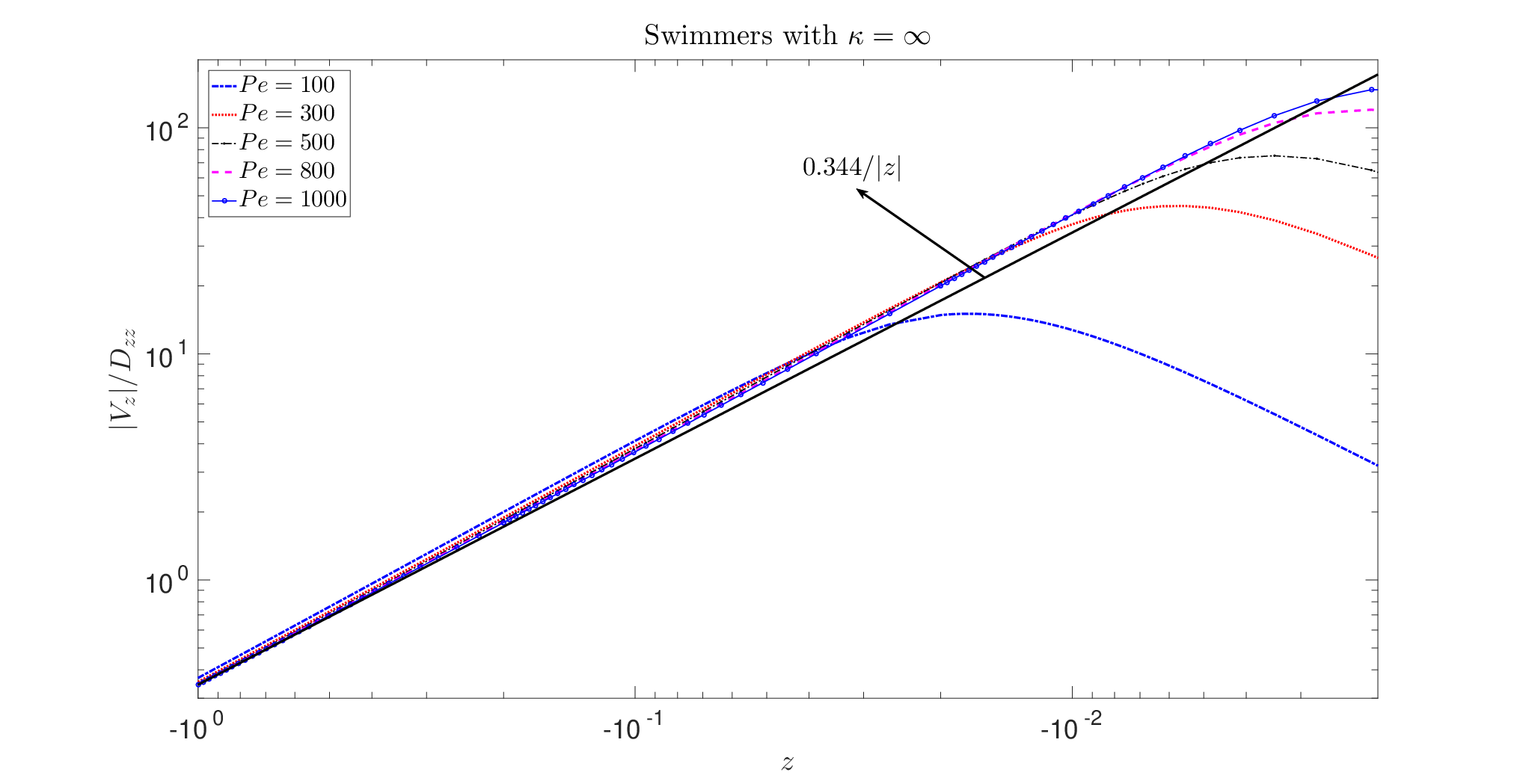
To further investigate the nature of the wallward migration, we plot, in figure 4, and at the channel wall as a function of Pe for and 15. For , both and , for any non-zero scale as for ; being determined by , the onset of this asymptotic scaling regime is postponed to a progressively larger with decreasing (not shown). For too, there is an intermediate range of ’s ( 3 to a little greater than 10) where the aforementioned scaling holds, but there is a deviation at larger ’s. As will be seen in §3.2, this deviation is a signature of the impending low-shear trapping regime. The observed scalings may be rationalized by noting that , where O is the swimming speed, projected along the gradient direction, of a swimmer in the large- orientation boundary layer, with an angular extent of O(), that forms around the flow direction [Hinch & Leal 1972a; Brenner 1974]; is the time over which rotary diffusion causes the swimmer orientation to fluctuate across the flow axis, leading to a de-correlation in its gradient-directed motion. The scaling for may be obtained by from arguments based on a gradient-directed biased random walk. One may write , where , represent the random walk jumps with frequencies , along the positive and negative gradient directions, respectively. Expressing the random walk jumps as the ratio of swimming velocity in that direction to the associated frequency, one has , where is the (dimensionless) gradient-projection of the swimmer mean free path. With a swimming velocity of O() and a decorrelation time of O(), one obtains . Using this leads to O.
The identical drift and diffusivity scalings above imply that the ratio is independent of for large , and hence, so is the concentration profile. We find , consistent with the scaling arguments above, with a constant of proportionality () of order unity. This leads to a large- functional form of the concentration profile given by . In figure 5, for , we compare the variation of against , for different . A fit to the large- variation away from the centerline leads to . From figure 2a, the swimmer concentration profiles are seen to approach the above -independent limiting form for . Although, the steady state profile is -independent, the time taken to attain steady state is of O() and diverges for . The limiting concentration profile is singular with a cusp at the centerline (). The cusp is, of course, an artefact of the limit. For any finite , the multiple scales analysis breaks down in an asymptotically small interval of O() in the vicinity of the centerline (keeping in mind our interpretation of as a swimmer Knudsen number, this layer in the vicinity of the centerline, where ballistic swimmer trajectories play an important role, may be termed a Knudsen layer in traditional kinetic theory parlance). Note that both the swimmer orientation distribution and concentration in this Knudsen layer may be influenced by the bound trajectories observed for deterministic swimmers observed in Zöttl & Stark 2013.
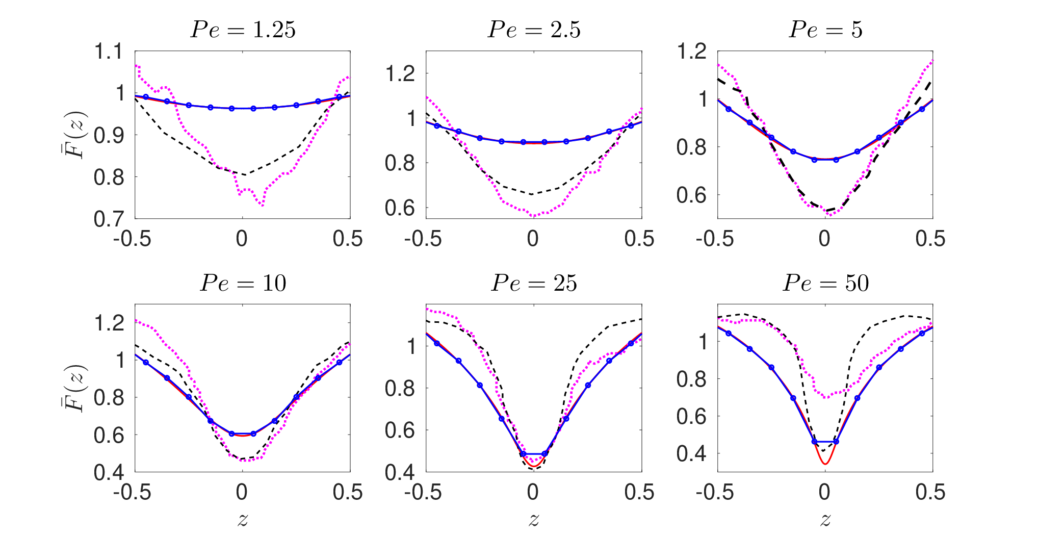
In figure 6, we compare our theoretical and simulation results (which are in mutual agreement regardless of ) with those reported in Rusconi et al. 2014b for . For the three smallest ’s (1.25, 2.5 and 5), our theory under predicts the inhomogeneity compared to the experiments. There is improved agreement at , and again, at the highest ’s (25 and 50), the disagreement with the experiments widens. The disagreement at the two highest ’s, we believe, is because the experiments [Rusconi et al. 2014b] sampled under-developed concentration profiles. The channel length available for development of the concentration profile corresponds to a single arm of the serpentine tube used in the experiments, and is approximately 5 cm (note that, in light of the later experiments by Aronson and co-workers [Sokolov & Aranson 2016; Sokolov et al. 2018, in a curvilinear geometry, it is likely that the bends of the serpentine tube significantly disrupt the concentration profile developed in the straight sections). At large , the entrance length may be estimated based on the time scale for attainment of steady state mentioned above, and is O(). Here, is the average suspension velocity and is the the mean shear rate; the numerical pre-factor (0.06) in the above estimate is determined from the Langevin simulations. Based on this estimate, and using m, m , [Rusconi et al. 2014b], the entrance length at is 1.4m! For , the entrance length is about 3 cm, which is smaller than the aforementioned length of a straight section. This would suggest that the measured profile at is indeed fully developed. The fact that our simulation results at intermediate times closely match shapes of the experimental profiles at two largest ’s (not shown here), reinforces the above assertion of the latter profiles not being fully developed ones. A second reason for deviation from theory could be the role of wall interactions, which are not included in the present analysis, the focus here being on bulk mechanisms for migration. Theory and simulations based on image induced interactions of pusher-type swimmers, and experiments on smooth swimming bacterial strains have shown swimmer accumulation at the boundaries in the absence of an imposed flow [Berke et al. 2008; Lauga & Powers 2009; Chilukuri et al. 2014]. However, in the present context we expect this effect to only have a minor influence for two reasons. First, the time scale O(), over which the wall interaction is significant, is comparable to the time scale for orientation decorrelation of O for wild-type swimmers under consideration, and the latter acts to disrupt any hydrodynamically induced accumulation for small ; in contrast, for the smooth swimmers used in Berke et al. 2008, the decorrelation time scale given by O(), was greater by at least two orders of magnitude. At large , rotary diffusion induced decorrelation is weak, and one then has a sustained image-induced interaction between nearly flow-aligned swimmers. Wall interactions, even in this case, are expected to only induce a concentration enhancement within a region of O() from the walls. Using Brownian dynamics simulations for a confined channel geometry, with hydrodynamic interactions between the swimmers and wall included, Chilukuri et al. 2014 showed that wall accumulation is indeed localized to the immediate vicinity of boundaries, consistent with the above arguments, and that this accumulation is further suppressed when the swimmers are subject to a pressure driven channel flow. Given that the observations of Rusconi et al. 2014b and Barry et al. 2015 were in the central portion of the channel, one expects the swimmer concentration to remain largely unaffected by wall interactions.
The disparity at the smallest ’s, pointed out above, could be due to multiple reasons. First is the possibility of the assumption , underlying the multiple scales analysis, breaking down. Based on the microchannel geometry and the known mean free path for B. subtilis (estimated from the decorrelation time that is in turn inferred from the measured translational diffusivities), in the experiments of Rusconi et al. 2014b. Our simulations, which are not limited by the small assumption, agree well with theory even for , ruling out the lack of smallness of the swimmer Knudsen number as a cause of theory-experiment incongruity. Note that the issue of not being small enough is not relevant to the largest ’s since the stronger flow alignment of the swimmers with the unaltered decorrelation time implies that the projection of the mean free path in the cross-stream direction shrinks with increasing , increasing the range of validity of the multiple scales analysis. For the high-shear trapping regime considered in this section, the effective Knudsen number is , the exponent reflecting the degree of swimmer alignment in the orientation boundary layer; for low-shear trapping examined next, for large . Next, it is also possible that the particular choice of the swimming mechanism determines the detailed concentration profile; for instance, there might be a significant difference between the degree of inhomogeneity in the swimmer concentration between RTP’s and ABP’s. As explained in the introduction, the former involves the swimmer undergoing a sudden large change in its orientation during tumbles [Berg 1993; Berg 2008], while the latter involves continuous small amplitude fluctuations in their orientation. Our Langevin simulations do suggest a greater inhomogeneity for RTP’s than ABP’s at the smallest ’s, with this difference diminishing in magnitude with increasing . Thus, the difference between the swimming mechanism of B. subtilis, relative to the pure ABP-dynamics assumed in the theoretical framework here, may cause the discrepancy between experiment and theory at the smallest ’s (the Rusconi et al. 2014b experiments only measured the translation diffusivities, and do not therefore have detailed information with regard to the relative importance of tumbling vis-a-vis rotary diffusion). The sensitivity of the shear induced migration pattern to the swimming mechanism does deserve a more detailed study, and this will be reported in a future effort.
3.2 Swimmer migration towards the channel centerline - Low-shear trapping
Figure 7 shows the -dependent swimmer concentration profiles for a range of swimmer aspect ratios, including the case examined earlier (now over a larger range in extending upto 2500). For small to intermediate , one observes high-shear trapping regardless of , consistent with the results of the small- analysis, and as seen before, the corresponding concentration profiles exhibit a single minimum at the centerline. At large , however, there is a qualitative change with the concentration profiles now exhibiting a pair of maxima symmetrically disposed about the centerline; the maxima increase in amplitude, while converging towards the centerline with increasing (consistent with the earlier finite element computations of Bearon & Hazel 2015). The aforementioned transition occurs across a -dependent threshold . The Langevin simulations reinforce the existence of the transition in the concentration profiles; as shown in figure 7a, the profile at 4 exhibits a depletion of swimmers near the centerline, and the one at 40 exhibits a near-center excess.
To understand the transition from high-shear to low-shear trapping with increasing , in figure 8, we plot and , appropriately scaled, against for and for the ’s in figure 7. From figures 8c and d, is seen to undergo a change in sign with increasing (the associated zero-crossing appears as a sharp dip in the log-log plots), which is responsible for the reversal in migration. For ’s smaller than that corresponding to the zero-crossing (of ), swimmers migrate towards the walls; for larger ’s, swimmers migrate towards the centerline, leading to a low-shear trapping behavior. It is important to note that the reversal in migration is actually a function of , occurring for exceeding a -dependent threshold. This is confirmed in figure 9, where the plots of the diffusivity and drift against for , at different transverse locations (), confirm the onset of the asymptotic O() scaling regime at progressively larger for approaching the centerline (figures 9a and b). The reversal in drift is also delayed at locations closer to the channel centerline, with the earliest reversal occurring at the walls (the one shown in figure 9b). To further confirm the role of (rather than ), in figures 9c and d, and are plotted as a function of . This collapses the different curves into a single one, and also collapses the zero-crossings of the different curves onto a single location corresponding to a critical . Since always becomes arbitrarily small close enough to the centerline, there is always a region close to the centerline, regardless of , where swimmers continue to exhibit a wallward migration. This leads to the non-monotonicity, with a pair of maxima bracketing a central dip in the concentration profiles shown in figure 7; thus, the central portions of all the profiles in figure 7, corresponding to low-shear trapping, still resemble the depletion profiles seen earlier is §3.1. It is only the limiting excess profile, for , where swimmers migrate towards the centerline regardless of (this singular profile is subject to the limitations of the multiple scales analysis mentioned earlier in §3.1). As evident from figure 8, for any finite , both and exhibit an O() scaling in the low-shear trapping regime that emerges for sufficiently large , although for the larger values of (10 and 15), there is the emergence of an intermediate scaling regime (evident from figures 8a and c) where , already seen in §3.1. Thus, is the only case where the O() scaling regime persists in the limit , as indicated by the black-dashed lines in figure 8. Infinitely slender swimmers therefore represent a singular limit with regard to shear induced migration behavior. Of course, for large enough ’s, the corresponding to the transition to low-shear trapping may be large enough as to be numerically inaccessible. This is seen to be the case in figure 8b for =15, and in figure 8d for both and ; owing to the zero-crossing, it takes a larger for the drift to conform to the eventual O() scaling behavior.
From the results presented thus far, it is seen that the transition from high to low-shear trapping occurs at a threshold of order unity for ’s of order unity. For large , the cross-over is asymptotically large, and marks a transition from O() to an O() scaling regime for the drift and diffusivity coefficients (see figure 9). From classical work on the orientation dynamics of passive anisotropic Brownian particles in a simple shear flow [ Leal & Hinch 1971; Hinch & Leal 1972a; Brenner 1974], the former scaling regime implies the localization of the swimmer orientation distribution in an O() boundary layer around the flow direction where there is a balance between the rotary diffusion and flow-induced rotation. In contrast, when flow-induced rotation along Jeffery orbits occurs on a time scale much shorter than rotary diffusion, the latter acts as a regular perturbation; there is no orientational boundary layer, and one expects a scaling regime involving an integral powers of . Thus, the aforementioned cross-over must correspond to the point where the flow-induced (Jeffery) rotation, on a time scale of O() is comparable to that characterizing rotary diffusion of O(); this leads to O() for (this scaling is confirmed in §3.3.2, where we demarcate high and low-shear trapping on the plane). Now, at leading order, one has purely flow induced Jeffery rotations of the swimmer, with an orbital time period . The Jeffery rotations coupled with swimming lead to a swimmer trajectory, that along the cross-stream direction, has a bounded but oscillatory character with an amplitude of O(). Rotary diffusion disrupts the exact periodicity of the leading order trajectory, causing an occasional slip of O(). These random displacements in the -direction, occurring over a time scale of O(), leads to a which may be written as O(), confirming the scaling behavior observed in the low-shear trapping regime; here, is the mean square displacement of the swimmer in the gradient direction. Note that, for large , swimmers spend an O time remaining nearly aligned with the flow axis at an angle of O(). This leads to the same estimate for as above, but a faster decorrelation rate of O() (since rotary diffusion only has to induce an angular displacement of O()), leading to a scaling for of O(). Based on the biased random walk argument as mentioned in §3.1, we can express . Now, for swimmers with of O(1), using , we obtain O(). The drift and diffusivity scalings above are broadly consistent with those obtained in figure 8b.


For large , similar to the high-shear trapping case, and exhibit the same O() scaling, their ratio being independent of and of the form , where is now a function of . One therefore expects a limiting -independent profile of the form ; note that, for any finite , this profile breaks down in the vicinity of the centerline, where the actual finite- profiles exhibit a dip, corresponding to the onset of depletion (wallward migration) at small . Since for low-shear trapping (owing to the sign-reversal of the drift), this limiting profile has a diverging concentration at the centerline. For , , and the associated limiting profile compares well to the numerically computed ones in figure 7a. An interesting consequence of the change in sign of , leading to low-shear trapping, is that the aforementioned limiting profile fails to be integrable for (this wasn’t an issue in the high-shear trapping case, since the swimmer concentration in all profiles, including the one corresponding to , is bounded below by zero). We find to equal this threshold value (-1) for , and decrease further for larger . The implication of the non-integrability above is that, for , the swimmer concentration profiles must exhibit a ‘centerline collapse’ in the limit ; in other words, . Figure 10 shows the variation of swimmer concentration at the wall against for the aspect ratios considered in figure 7. For 1.25, the near-wall swimmer concentration approaches a finite limiting value . For , however, the near-wall swimmer concentration decreases monotonically to zero for , in accordance with the centerline-collapse hypothesized above. The slope characterizing this decrease appears to increase with increasing , implying that the collapse increases in intensity for larger (for 15, the numerics have not accessed the asymptotic regime yet). The -dependence of the collapse does suggest that the drift and diffusivity coefficients must scale differently with for . Scaling arguments presented above suggested that O in the low-shear trapping regime, and the large scaling of the drift must therefore differ from O() that would emerge from the biased-random-walk scaling above modified for . The large- scaling of the drift in this regime will be analyzed in detail in a future effort.
Unlike the rather intuitive picture underlying high-shear trapping (see figure 3 in §3.1), the physical mechanism underlying low-shear trapping is more subtle. Here, we present arguments that support migration of swimmers towards the centerline at large , beginning from the orientation dynamics of swimmers in a local linear flow description, as shown in figure 11a. For the parabolic flow under consideration, the local linear approximation yields a simple shear flow with a shear rate that decreases from a maximum at the wall to zero at the centerline. For any finite , and sufficiently large ( for of O(1); for ), swimmers at any non-zero execute Jeffery rotations at leading order, with a time period commensurate with the -dependent shear rate of the simple shear flow above. The resulting distribution of azimuthal angles within any Jeffery orbit is symmetrical about the flow direction (as first shown by Leal & Hinch 1971, the distribution across the orbits is still controlled by asymptotically weak rotary diffusion, although this doesn’t affect the argument for the direction of drift given below). At the next order, O(), rotary diffusion breaks the aforementioned symmetry, leading to an excess of orientations in the extensional quadrants, and an equal and opposite deficit in the compressional ones (this antisymmetry is a consequence of Brownian motion being a weak but regular perturbation; in the singular case, relevant to the high-shear trapping regime, almost the entire swimmer probability is confined to the extensional quadrants). The aforementioned distributions at O(1) and O() are sketched in figure 11a. Owing to the decrease of , the amplitudes of the excess and deficit above increase as one moves away from the wall. The lower figure in 11b contains sketches of the local simple shear flows at three different -locations, with the local excess and deficit in orientations in accordance with the arguments above (the swimmer lengths shown denote the amplitude of the excess or deficit). This picture may now be used to argue, in a quadrant-wise manner, for the swimming-induced changes the orientation distribution. At any , in quadrant I, lesser excess swims in from the stronger shear flow below, and a greater excess exits into the weaker shear flow above; in quadrant III, the exact opposite occurs. Similarly, in quadrant II (IV), a greater (lesser) deficit exits into the weaker (stronger) shear flow above (below), with a lesser (greater) deficit swimming in from the stronger (weaker) shear flow below (above), leading to a net excess (deficit) of swimmers. As a result, there is a swimming-induced source of probability in quadrants II and III, and a sink in quadrants I and IV. In turn, this implies that the azimuthal flux of probability will, on a clockwise traversal, increase through quadrants II and III, and then decrease through IV and I. Accounting for the depleted orientation probability in the compressional quadrants (II and IV), this flux-profile leads to an excess of swimmers in quadrants I and II, implying a net drift towards low-shear regions. This migration towards the low-shear regions continues till the swimmers reach sufficiently close to the channel center where eventually falls below . From this location onward, and up until the centerline, the swimmers revert to a wallward migration. Therefore, the steady state concentration profile is such that it exhibits a maximum at a location intermediate between the centerline and the wall, with this location shifting towards the centerline with increasing .

3.3 Depletion index and the migration portrait
Having discussed the two kinds of migration patterns mentioned above, in §3.3.1, we quantify the same in terms of the depletion index , a non-dimensional measure of the inhomogeneity of the swimmer concentration field: corresponds to high-shear (low-shear) trapping. Next, in §3.3.2, we organize the migration behavior on a plane (for small ), thereby delineating the regimes of high-shear and low-shear trapping across a numerically determined phase boundary.
3.3.1 The depletion index (DI)

We define , where represents the area under the initial uniform distribution from the wall up to its intersection with the steady state swimmer concentration profile (), denotes the analogously defined area under the steady state profile from the channel wall to and is the total area under either profile. For depletion profiles, conservation of swimmer number does imply that equality of areas between the wall and , and between and centerline. To analyze swimmer migration at large , is plotted against for swimmers of different aspect ratios in figure 12. The plot discriminates between high () and low-shear trapping behavior (), and in addition, helps differentiate between centerline-collapse ( for for ) and non-collapse ( approaches a finite value as for for ) behavior within the low-shear trapping regime. Figure 12 clearly illustrates the singular nature of infinitely slender swimmers. For , plateaus at a finite value () for . In contrast, for any finite approaches zero in the same limit, and the rate of approach, rather counter intuitively, increases with increasing . For large ’s, this accelerated approach towards the origin begins after an intermediate extended plateau with (the same plateau value as for ). Note that Rusconi et al. 2014b, likely motivated by experimental considerations, had defined depletion index () based on the area between the actual and uniform profile in the central half width of the channel. The general character of figure 12 is, however, unchanged regardless of the definition.
It is worth reiterating the behavior of the depletion index, , as a function of the swimmer aspect ratio starting from infinitely slender swimmers. Regardless of , starts from 100 for . For , increases with increasing , approaching a constant () for . For large but finite , again increases with increasing , asymptoting to the aforementioned plateau value in the range , and thereafter, decreases rapidly with further increase in . This behavior continues with decreasing , with the -interval corresponding to the intermediate plateau above progressively shrinking in extent, and the eventual rate of approach to zero at large also decreasing with decreasing . For the ABP’s examined here, this trend continues until a critical aspect ratio of approximately 2, when approaches zero only at a logarithmic rate for large ; that is, for , is O() for . For , approaches a finite positive plateau (less than 100) for , with this plateau value approaching 100 as approaches unity (spherical swimmers). It is worth noting that the infinite-aspect-ratio assumption is used routinely in the rheological context, when analyzing swimmers suspensions, and generally yields good agreement in between experiments and theory [Saintillan 2010a; Saintillan 2010b; López et al. 2015; Nambiar et al. 2017; Nambiar et al. 2019b]. In the present context, however, even for moderately large aspect ratios, (relevant in the biological context), at large enough , the swimmers can, in fact, end up being trapped in the low-shear regions. Thus, the effective aspect ratio parameter appears to be of considerable importance in the context of shear-induced migration.
Although our theoretical predictions and simulations are in mutual agreement, there is nevertheless a disagreement with the experiments of Rusconi et al. 2014b; aspects of this disagreement were already elaborated on in §3.1. In order to illustrate the discrepancy, we have plotted , against , as an inset in figure 12 for . While the disagreement appears a matter of detail, in the sense that the in the experiments peaks at a smaller ( 10), and starts decreasing earlier, it is not! The interpretation in the original experiments was that the would asymptote to zero for larger . As discussed earlier, this decay of the to zero, implying the approach of the swimmer concentration profile towards homogeneity, is a consequence of the experimental profiles not being fully developed on account of the limited residence time (ironically enough, the apparent peaking of the at a finite shear rate in these experiments was motivation for subsequent experiments by Aronson and co-workers [Sokolov & Aranson 2016; Sokolov et al. 2018], in a curvilinear geometry, where the inhomogeneity in swimmer concentration was argued to persist at infinite , albeit for entirely different reasons). As argued above, the does not approach zero, for any aspect ratio, in the limit of large . Thus, the apparent decay of the theoretical is a signature of the transition to a low-shear trapping regime, and the theoretical will eventually asymptote to -1, for the aspect ratio of 10 considered (which allows for a centerline collapse as ).
3.3.2 The migration portrait

Figure 13 organizes the high-shear and low-shear trapping regimes on the plane, with an approximate boundary separating the two. We differentiate the high-shear trapping from the low-shear trapping, based on the slope of the swimmer concentration profile at the channel wall. Across the phase boundary, there is a change in sign of this slope, arising from the reversal in the drift; see figure 8 in §3.2 (note that this criterion suffices in the present context where the focus is on shear induced migration in the bulk; inclusion of wall interactions, would require a modification of this criterion. This is not an issue for comparison with the experiments, however, since the swimmer concentrations were monitored well away from the boundaries). The large aspect ratio asymptote for the aforementioned boundary between the two trapping regimes has already been determined based on the scaling arguments given in §3.2, and is of the form ; the pre-factor 0.07 given in figure 13 is determined from a best fit for the curve separating the numerically determined depletion and excess profiles. Now, due to the absence of any preferential alignment under shear, spherical-swimmer concentration profiles are homogeneous regardless of , in the dilute non-interacting regime under consideration. Nevertheless, the small but finite inhomogeneity that arises in the limit can transform from a near-center depletion to a near-center excess at a finite . This is indeed the case, and based on an expansion of the swimmer probability density in the small Bretherton constant , as , one finds (see appendix C). Therefore, as , ABP’s exhibit high and low-shear trapping profiles across , with the analytical forms for the latter profiles also exhibiting the characteristic pair of maxima on either side of the centerline, already seen in the numerical profiles. This transition for near-spherical swimmers has again been validated using numerical predictions based on the multiple scales analysis, and Langevin simulations.
Also shown in figure 13 are the results from the experiments of Barry et al. 2015 corresponding to both high-shear and low-shear trapping of the phytoplankton algae Heterosigma and Dunaliella. The effective swimmer aspect ratios () in the experiments were determined from a best fit of the theoretical orientation distribution, obtained by solving the Fokker-Planck equation with as a fitting parameter, with the experimentally determined one. Note that the ’s determined in the manner above were functions of , implying that the swimmer shape changed on account of the shear induced deformation. Based on the concentration profiles and depletion index plots () reported in Barry et al. 2015, for , Heterosigma exhibit high-shear trapping, whereas, Dunaliella, show high-shear trapping till but transition to low-shear trapping at at . Similar to the observation of Barry et al. 2015, for the algae Dunaliella, we too observed the transition from the high-shear to low-shear trapping with increase in . The experimental data points are thus consistent with the trapping regimes identified in figure 13, and this consistency serves as an important validation of the analysis and arguments presented here.
4 Conclusions
Motivated by recent microfluidic experiments [Rusconi et al. 2014b; Barry et al. 2015], in this work we have used both theory and simulations to systematically study shear induced migration in a dilute suspension of microswimmers subject to a plane Poiseuille flow in a wide channel. On the theoretical front, we have used the method of multiple time scales to derive a drift-diffusion equation governing the steady state cross-stream swimmer concentration profile. Based on the swimmer geometry, as characterized by its equivalent aspect ratio , and a rotary Péclet number that characterizes the relative efficiency of stochastic reorientation and flow-induced rotation, we delineate high-shear and low-shear trapping regimes. Our theoretical predictions are reinforced by the results of Langevin simulations, and establish for the first time, the existence of a low-shear trapping regime at sufficient large for any finite . The transition from high-shear to low-shear trapping appears consistent with the experimental data available from Barry et al. 2015; the biflagellated algal species, Chlamydomonas and Dunaliella, used in the experiments exhibit a low-shear trapping regime at high shear rates, with the latter species going through a high-shear trapping regime at lower shear rates. The approach of microswimmers to any surface is the first step towards colonization and biofilm formation. The existence of both high- and low-shear trapping regimes points to the possibility of manipulating fluid shear to possibly reinforce or retard biofilm formation; thus, the high and low-shear trapping regimes in figure 13 may perhaps be equivalently interpreted as regimes where hydrodynamics favors and opposes biofilm formation. A richer range of concentration patterns and dynamical regimes, relative to those identified earlier in Rusconi et al. 2014b and Bearon & Hazel 2015, is expected in the presence of an ambient chemical gradient that causes chemotactic swimmers to drift towards a boundary (as a possible precursor for biofilm formation), while a high- shear drives migration in the opposite direction. This particular aspect will be pursued in the near future.
The organization of shear induced migration of active swimmers as a phase portrait has important implications. The fact that swimmers on either side of the phase boundary in figure 13 migrate in opposite directions allows, in principle, for a microfluidic shape sorter ( being a surrogate for the swimmer shape). A shape-based sorting might be feasible in the low-shear trapping regime alone by exploiting the centerline collapse (for ) that occurs for , (application of the multiple scales analysis shows that results for the plane Poiseuille flow derived herein, including the threshold aspect ratio for centerline collapse, directly carry over to the pipe Poiseuille case). A second interesting implication of the centerline collapse is for the dispersion of microswimmers in the flow direction (this has been examined, in the limit of confined channels, by Chilukuri et al. 2015). It is known from classical Taylor-dispersion theory that, in the limit where the microswimmers uniformly sample the channel cross-section, the mean square displacement in the flow direction scales as O(), and therefore, increases with increasing ; here, , is the Péclet number based on the swimmer translational diffusivity. For large-aspect-ratio microswimmers in the low-shear trapping regime identified here, the extent of the channel cross-section sampled decreases sharply with increasing (or increasing with fixed), pointing to a possible non-trivial scaling of the flow-induced dispersion in the limit of large .
An interesting consequence of the detailed analysis here is the remarkable sensitivity of the shear induced migration to subtle changes in the orientation dynamics. These differences in orientation dynamics were originally identified in the context of passive anisotropic particles, in a series of studies by Hinch and Leal [Leal & Hinch 1971; Hinch & Leal 1972a; Leal & Hinch 1972; Hinch & Leal 1972b; Leal & Hinch 1973; Hinch & Leal 1973], who were motivated by the need to understand the subtle role of weak Brownian motion in strong shearing flows, and its implications for suspension rheology. In fact, they turn out to much more crucial for active particles, being responsible for the onset of a low-shear trapping regime! Indeed, Nitsche & Hinch 1997 have previously used the method of multiple scales to examine shear induced migration in a dilute suspension of passive anisotropic particles. Such particles do exhibit a high-shear trapping on account of the anisotropy of the mobility, and thence, the Brownian diffusivity. The trapping arises because of the lower transverse diffusivity(mobility) of flow-aligned particles close to the walls, but it is a relatively weak effect owing to the mobility anisotropy (defined as the ratio of the longitudinal to the transverse mobility coefficients) saturating at 2 even for infinitely slender particles; experiments on fiber suspensions have failed to observe the predicted high-shear trapping [Nitsche & Hinch 1997] at lower volume fractions [Strednak et al. 2018]. Since the Brownian mobility, and therefore, the diffusivity at any non-zero , asymptotes to a finite value for , the concentration profile must become spatially homogeneous in this limit; in sharp contrast to the active case examined here.
Assuming an independent source of translational diffusion (thermal or otherwise), with components and along and transverse to the flow direction, in addition to the translational diffusion arising from swimming activity considered here, one may use scaling arguments to predict the transition from the active shear induced migration analyzed here to the migration behavior of passive anisotropic particles analyzed by Nitsche & Hinch 1997. This transition is most relevant to large aspect ratio swimmers, since swimmers with moderate would have transitioned to their asymptotic low-shear trapping regime (collapse or non-collapse) at fairly moderate values of . To estimate the threshold for the active-passive transition, we balance with the high- asymptote for the translational diffusivity in the high-shear trapping regime, given by (see figure 9); we consider the diffusivity at the wall, which gives an upper bound for the threshold. The balance yields . Equating this threshold to , one obtains a threshold aspect ratio (as must be the case, the same expressions for and result on using corresponding to the low-shear trapping regime). The significance of above is that the concentration profiles for swimmers with would transition to homogeneity (for ) directly from the high-shear trapping regime, while the concentration profiles for swimmers with will asymptote to homogeneity from the low-shear trapping regime. When has a thermal origin, using the familiar Stokes-Einstein expression with the translational mobility for a slender body, one has [Dhont 1996] with being the Boltzmann constant, being the temperature, and being the suspension viscosity. This yields O(10) for m, m, , and for the aqueous medium used to suspend the microorganisms [Rusconi et al. 2014b; López et al. 2015]. Thus, the B. subtilis in Rusconi et al. 2014b experiments are expected to transition to a passive-migration behavior at a that is about two orders of magnitude higher than the highest sampled in the experiments. The larger algae used in Barry et al. 2015 should yield much larger values.
Finally, it must be noted that figure 13 depicts migration behavior specifically for ABP’s. One expects a similar phase portrait for other swimmer types (RTP’s, for instance), although the aforementioned sensitivity to the orientation dynamics obviously points to different scalings for the phase boundary (and a different threshold aspect ratio for a possible centerline collapse). Such an analysis, and its implications towards flow-based separation of microswimmers, with different swimming characteristics, will be reported separately.
Acknowledgements
L.N.Rao would like to thank Science and Engineering Research Board, India (Grant No. PDF/2017/002050) for the financial support.
Appendix A Numerical scheme for the swimmer probability densities and concentration profile.
In the following, we describe the numerical scheme adopted to evaluate the swimmer orientation probability densities and , at O(1) and O(), respectively, and thence the steady state swimmer concentration profile of (7), mentioned in §2.1. To solve (4), for , we use a spherical coordinate system with its polar axis aligned with the -axis (see figure 1). As a result, the components of the swimmer orientation vector are given by , , . The flow-induced rotation term in (4), , may now be written as:
Expressing () in terms of spherical harmonics, we have:
| (11) | |||||
Now, expanding
| (12) |
and substituting in (11), one may write:
| (13) |
where , represent the spherical harmonics and are the associated Legendre functions [Abramowitz & Stegun 1965] and .
Next, we substitute the expansion for above in the remaining terms of (4), with the tumbling kernel being given by [Subramanian & Koch 2009; Nambiar et al. 2017]; here, is the correlation parameter characterizing the tumbles, and represent the Legendre polynomial of the th degree, with argument being the cosine of the angles between the pre- and post-tumble operations. Further, employing the addition theorem of spherical harmonics and that [Abramowitz & Stegun 1965], (4) may finally be written as the following summation over the spherical harmonics:
| (14) | ||||
| (15) |
In the above equation, (from the conservation of swimmers during tumble events: ) and
| (16) |
Using the following identities in (15) [Doi & Edwards 1978; Messiah 1962]
and after simplification, we get:
| (17) |
where and .
Now, multiplying the above equation with the conjugate spherical harmonic , then integrating it over the unit sphere, and using the orthogonality of spherical harmonics, we obtain the following infinite sequence of linear equations for the ’s:
| (18) |
In the above equation, the Clebsch-Gordan coefficients
will be evaluated using the Racah formula [Arfken & Weber 1999; Doi & Edwards 1978; Messiah 1962].
Using and (12) in the following normalization condition (see §2.1)
| (19) |
we get
| (20) |
Substituting (20), in (18), we have:
| (21) |
An appropriately truncated version of (21) is solved numerically to obtain the ’s, subject to convergence of the orientation distribution.
Now substituting in the right hand side of (5), after simplification, we obtain:
| (22) |
To evaluate in the equation above, we first differentiate (4) with respect to :
| (23) |
Substituting for on the right hand side, using (12), and using the expansion
| (24) |
in (23), we get:
| (25) |
Differentiating (19) with respect to , using (24) and using the orthogonality of spherical harmonics, we get
| (26) |
Now, following a procedure analogous to that leading to (21), the sequence of linear equations governing the ’s in (25) may be written as:
| (27) |
where, and . One can solve the system of linear equations (27) to determine as a truncated version of (24).
To solve for in (5), on account of linearity, we first write:
| (28) |
and equating the coefficients of and on both sides, we get the following equations governing and :
| (29) | ||||
| (30) |
Expanding
| (31) |
| (32) |
using (28) in (19) and using the orthogonality of spherical harmonics, we get
| (33) |
From (12), (24), (19), (27), (31), (32), and following the numerical scheme adopted for solving (23), we obtain the unknown coefficients and .
Using (28), (31), (32) in (2.1), integrating over the orientation degrees of freedom and using (from (19)), we get the drift-diffusion equation describing the evolution of swimmer concentration profile
| (34) |
in terms of the slow time variable , and with the drift and diffusivity coefficients being defined by:
| (35) |
and
| (36) |
The drift-diffusion equation (34) appears as (7) in §2.1. The truncation in the above sequences of equations is such as to ensure converged values for the and . The truncated system has . For , and 4, reported in the manuscript, we chose ; for the other aspect ratios, we chose and 80 for and , respectively.
We calculate the steady state swimmer concentration profile satisfying (34), while imposing the zero-flux condition at boundaries, which leads to
| (37) |
at .
Appendix B Small- expansion for the swimmer concentration profile
Herein, we obtain closed form analytical expression for the swimmer concentration, to O(). The orientation probability density at each order (in ) in the multiple scales analysis (see §2.1) is further expanded in powers of to O(). Thus, the probability densities of O(1) ( in (4)), and at O() ( in (5)) are expanded to O(), with the imposition of the normalization condition: . Here and in §C, we choose a coordinate system different from the one used in §2.1 (figure 1), such that the polar () and azimuthal () angles are measured from the negative vorticity and flow axes, respectively. We first consider the probability density at leading order in the multiple scales analysis, and expand it about the isotropic orientation distribution, for , as:
| (40) |
with .
At successive orders in , we obtain:
| (41) | |||||
| (42) |
We solve (41) for , by using the modified Green’s function [Subramanian & Koch 2009] which satisfies:
| (43) |
where denotes the Dirac delta function in orientation space, with the forcing in (43) being a localized source at an orientation , together with a compensating uniformly distributed sink over the remainder of the unit sphere. The modified Green’s function result given in Subramanian & Koch 2009, derived for the rotary diffusion of swimmers can be easily generalized to the case of run-and-tumble plus rotary diffusion, so as to arrive at the following expression for as:
| (44) |
where
Using the expression for in (44), the orientation probability density , at O(), may be written as:
| (45) |
Similarly, using the modified Green’s function, the solution of (42) may also be expressed as:
| (46) |
Again, using (44), (45) in the above equation, expressing in terms of spherical harmonics, and using the orthogonality of the latter, we get:
| (47) |
From (40), (45) and (47), we obtain the small of the leading order orientation probability density, , to O() as:
| (48) |
Now, considering the equation at O(), given by (5), and expanding the unknown probability density as:
| (49) |
leads to the following three equations at successive orders in :
| (50) | |||||
| (52) |
The solutions of (50) and (B) may again be expressed as a convolution involving the modified Greens function. Using the modified Green’s function (44) and in (50), we have:
| (53) |
Using (45) for , (53) for , and the modified Green’s function (44), the unknown probability density in (B) can be expressed as:
| (54) | |||||
Similarly, using (47) for , (54) for and the modified Green’s function (44), the unknown probability density in (52) can be expressed as:
| (55) |
In the above equation, we only mention the coefficients of , since only these contribute to the drift, diffusivity, and hence the swimmer concentration profile (see (57) below).
Considering (2.1), integrating over the orientation degrees of freedom and using the normalization condition (see (19)), we get:
| (56) |
Expressing in terms of spherical harmonics, we have:
| (57) |
From orthogonality, only the coefficients of , in and , survive. Substituting for , from (53), (54), (55), the shear rate profile for the parabolic flow, , and evaluating the orientation-space integrals, we get:
| (58) |
where
In (58), the odd orders in don’t contribute, as must be the case, so the concentration profile is invariant to flow reversal. We therefore expand the swimmer concentration as . Substituting this expansion in (58), imposing the zero-flux condition at the boundaries (), we get:
| (59) |
At successive orders in , we obtain:
| (60) | ||||
| (61) |
Using (60) in (61), the leading order inhomogeneity () is independent of the correction to the diffusivity and the O() drift alone dictates the inhomogeneity. It is nevertheless worth noting that exhibits a profile consistent with physical arguments - the fact that it is negative, and larger closer to the walls, where the transverse diffusivity is suppressed due to increasing flow alignment of the swimmer. Although not relevant to the steady state, will influence the transient evolution from a generic initial condition.
Solving (60) and (61) for and , while imposing the normalization condition of swimmer concentration , we get:
| (62) |
where
| (63) |
with as the Bretherton constant and being given by (44). The comparison of the numerical and the analytical profiles of for swimmers with () and for different is given in figure 2a (inset) of §3.1.
Appendix C Concentration profile for the near-spherical swimmers
In the following, we obtain an analytical expression for the swimmer concentration profile, for an arbitrary , but for near-spherical swimmers which correspond to an asymptotically small Bretherton constant (). As we did in §B, we start from the small- expansion of probability density () in the multiple scales analysis, and expand the probability densities at each order in , in (4) at O(1), and in (5) at O(), to O(), while also imposing the normalization condition: . To begin with, consider the governing equation (4) for :
| (64) |
where , , represent the rotation rates of the swimmer at O(1) and O(), respectively, due to the local ambient vorticity and rate of strain. In (64), for near-spherical swimmers, we expand in the parameter , about the spatially homogeneous isotropically oriented base state
| (65) |
At leading order, one obtains the isotropically oriented state of spherical swimmers that spin at a uniform rate with the ambient vorticity. Thus, . At O(), we have the following governing equation for :
| (66) |
To solve the above equation for , we again seek a modified Green’s function , that satisfies
| (67) |
Here, differs from , given by (43), in that it includes the effect of vorticity-induced rotation in addition to the orientation decorrelation due to rotary diffusion and run-and-tumble dynamics. Writing down the modified Green’s function as a series in spherical harmonics
| (68) |
substituting in (67), and following the procedure mentioned in appendix B, we obtain
| (69) |
where Note that the azimuthal degeneracy is broken by the presence of the -dependent flow contribution. The effect of this flow contribution is to decrease the translational swimmer diffusivity at large . For, large , the spherical swimmer rotates with a period of O(). The rotation and swimming lead to a mean free path of O(). Taken together with the decorrelation time of O(), this implies a scaling of for the gradient component of the diffusivity. Thus, the rapid rotation induced by the ambient vorticity leads to an asymptotically small translational diffusivity at large .
Using the convolution integral involving the modified Green’s function given by (68), one may write the O() swimmer probability density , governed by (66), in the following final form:
| (70) |
Next, considering the swimmer probability density at O() in the multiple scales analysis, and expanding in :
| (71) |
we obtain the following equations at successive orders in :
| (72) | ||||
As in §B, only the terms involving contribute to the diffusivity () and drift (). So for simplicity, we do not mention the coefficients of in (75). Integrating (2.1) over the orientation degrees of freedom and using (from (19)), we get:
| (76) |
Using (71), (74), (75), in the above equation and integrating, gives:
| (77) |
where
| (78) | ||||
| (79) | ||||
| (80) | ||||
| (81) |
In the above equation, scales as O() for large , consistent with the scaling arguments above. From (81), we see that the O() drift at the wall, for near-spherical swimmers, changes sign when . This may be rewritten as , whence, one obtains the threshold for drift reversal as: . This critical is mentioned in §3.3.2, and appears in the phase portrait in figure 13.
Now, to obtain the steady state swimmer concentration profile we expand
| (82) |
substituting in the normalization condition yields and
| (83) |
| (85) |
Thus from (82), (85) and using , we obtain the following steady state concentration profile for near-spherical swimmers:
| (86) |
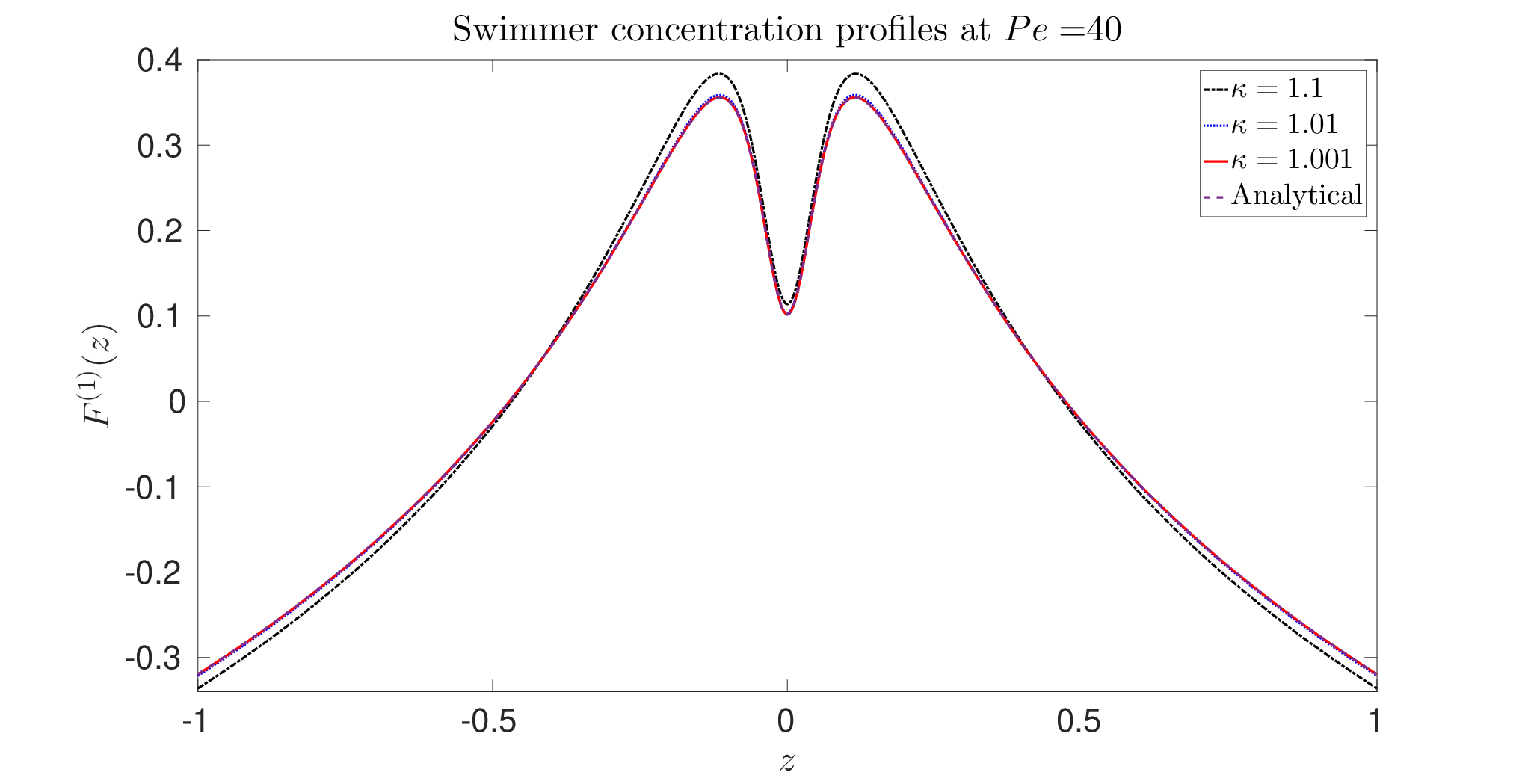
In figure 14, we compare the numerical and analytical results of for near-spherical swimmers at . Expectedly, the numerical profiles approach the analytical one for . More importantly, the spatial structure of the swimmer concentration profile is similar to that obtained for finite - a pair of concentration maxima on either side of the channel centerline.
References
- Abramowitz & Stegun (1965) Abramowitz, Milton & Stegun, Irene A 1965 Handbook of mathematical functions: with formulas, graphs, and mathematical tables, , vol. 55. Courier Corporation.
- Arfken & Weber (1999) Arfken, George B & Weber, Hans J 1999 Mathematical methods for physicists.
- Barry et al. (2015) Barry, Michael T, Rusconi, Roberto, Guasto, Jeffrey S & Stocker, Roman 2015 Shear-induced orientational dynamics and spatial heterogeneity in suspensions of motile phytoplankton. Journal of The Royal Society Interface 12 (112), 20150791.
- Bearon & Hazel (2015) Bearon, RN & Hazel, AL 2015 The trapping in high-shear regions of slender bacteria undergoing chemotaxis in a channel. Journal of Fluid Mechanics 771.
- Bechtel & Khair (2017) Bechtel, Toni M & Khair, Aditya S 2017 Linear viscoelasticity of a dilute active suspension. Rheologica Acta 56 (2), 149–160.
- Berg (1993) Berg, Howard C 1993 Random walks in biology. Princeton University Press.
- Berg (2008) Berg, Howard C 2008 E. coli in Motion. Springer Science & Business Media.
- Berke et al. (2008) Berke, Allison P, Turner, Linda, Berg, Howard C & Lauga, Eric 2008 Hydrodynamic attraction of swimming microorganisms by surfaces. Physical Review Letters 101 (3), 038102.
- Brennen & Winet (1977) Brennen, Christopher & Winet, Howard 1977 Fluid mechanics of propulsion by cilia and flagella. Annual Review of Fluid Mechanics 9 (1), 339–398.
- Brenner (1974) Brenner, H 1974 Rheology of a dilute suspension of axisymmetric brownian particles. International Journal of Multiphase Flow 1 (2), 195–341.
- Chaturvedi et al. (2010) Chaturvedi, Neetu, Hong, Yiying, Sen, Ayusman & Velegol, Darrell 2010 Magnetic enhancement of phototaxing catalytic motors. Langmuir 26 (9), 6308–6313.
- Chilukuri et al. (2014) Chilukuri, Sandeep, Collins, Cynthia H & Underhill, Patrick T 2014 Impact of external flow on the dynamics of swimming microorganisms near surfaces. Journal of Physics: Condensed Matter 26 (11), 115101.
- Chilukuri et al. (2015) Chilukuri, Sandeep, Collins, Cynthia H & Underhill, Patrick T 2015 Dispersion of flagellated swimming microorganisms in planar poiseuille flow. Physics of Fluids 27 (3), 031902.
- Darnton et al. (2007) Darnton, Nicholas C, Turner, Linda, Rojevsky, Svetlana & Berg, Howard C 2007 On torque and tumbling in swimming escherichia coli. Journal of bacteriology 189 (5), 1756–1764.
- Das & Lauga (2018) Das, Debasish & Lauga, Eric 2018 Computing the motor torque of escherichia coli. Soft matter 14 (29), 5955–5967.
- Dhont (1996) Dhont, Jan KG 1996 An introduction to dynamics of colloids, , vol. 2. Elsevier.
- Doi & Edwards (1978) Doi, Masao & Edwards, Sam F 1978 Dynamics of rod-like macromolecules in concentrated solution. part 2. Journal of the Chemical Society, Faraday Transactions 2: Molecular and Chemical Physics 74, 918–932.
- Dombrowski et al. (2004) Dombrowski, Christopher, Cisneros, Luis, Chatkaew, Sunita, Goldstein, Raymond E & Kessler, John O 2004 Self-concentration and large-scale coherence in bacterial dynamics. Physical review letters 93 (9), 098103.
- Ebbens et al. (2014) Ebbens, S, Gregory, DA, Dunderdale, G, Howse, JR, Ibrahim, Y, Liverpool, TB & Golestanian, R 2014 Electrokinetic effects in catalytic platinum-insulator janus swimmers. EPL (Europhysics Letters) 106 (5), 58003.
- Elgeti et al. (2015) Elgeti, Jens, Winkler, Roland G & Gompper, Gerhard 2015 Physics of microswimmers—single particle motion and collective behavior: a review. Reports on progress in physics 78 (5), 056601.
- Ezhilan & Saintillan (2015) Ezhilan, Barath & Saintillan, David 2015 Transport of a dilute active suspension in pressure-driven channel flow. Journal of Fluid Mechanics 777, 482–522.
- Fischer & Ghosh (2011) Fischer, Peer & Ghosh, Ambarish 2011 Magnetically actuated propulsion at low reynolds numbers: towards nanoscale control. Nanoscale 3 (2), 557–563.
- Fu et al. (2012) Fu, Henry C, Powers, Thomas R, Stocker, Roman & others 2012 Bacterial rheotaxis. Proceedings of the National Academy of Sciences p. 201120955.
- Gadala-Maria & Acrivos (1980) Gadala-Maria, F & Acrivos, Andreas 1980 Shear-induced structure in a concentrated suspension of solid spheres. Journal of Rheology 24 (6), 799–814.
- Ghosh et al. (2012) Ghosh, Abhijit, Samuel, Joseph & Sinha, Supurna 2012 A “gaussian” for diffusion on the sphere. EPL (Europhysics Letters) 98 (3), 30003.
- Gray & Hancock (1955) Gray, James & Hancock, GJ 1955 The propulsion of sea-urchin spermatozoa. Journal of Experimental Biology 32 (4), 802–814.
- Guasto et al. (2012) Guasto, Jeffrey S, Rusconi, Roberto & Stocker, Roman 2012 Fluid mechanics of planktonic microorganisms. Annual Review of Fluid Mechanics 44, 373–400.
- Guo et al. (2018) Guo, Shuo, Samanta, Devranjan, Peng, Yi, Xu, Xinliang & Cheng, Xiang 2018 Symmetric shear banding and swarming vortices in bacterial superfluids. Proceedings of the National Academy of Sciences 115 (28), 7212–7217.
- Hancock (1953) Hancock, GJ 1953 The self-propulsion of microscopic organisms through liquids. Proceedings of the Royal Society of London. Series A. Mathematical and Physical Sciences 217 (1128), 96–121.
- Hinch & Leal (1972a) Hinch, EJ & Leal, LG 1972a The effect of brownian motion on the rheological properties of a suspension of non-spherical particles. Journal of Fluid Mechanics 52 (4), 683–712.
- Hinch & Leal (1972b) Hinch, EJ & Leal, LG 1972b Note on the rheology of a dilute suspension of dipolar spheres with weak brownian couples. Journal of Fluid Mechanics 56 (4), 803–813.
- Hinch & Leal (1973) Hinch, EJ & Leal, LG 1973 Time-dependent shear flows of a suspension of particles with weak brownian rotations. Journal of Fluid Mechanics 57 (4), 753–767.
- Kasyap & Koch (2012) Kasyap, TV & Koch, Donald L 2012 Chemotaxis driven instability of a confined bacterial suspension. Physical review letters 108 (3), 038101.
- Kasyap & Koch (2014) Kasyap, TV & Koch, Donald L 2014 Instability of an inhomogeneous bacterial suspension subjected to a chemo-attractant gradient. Journal of Fluid Mechanics 741, 619–657.
- Kim et al. (2014) Kim, Minyoung Kevin, Drescher, Knut, Pak, On Shun, Bassler, Bonnie L & Stone, Howard A 2014 Filaments in curved streamlines: rapid formation of staphylococcus aureus biofilm streamers. New journal of physics 16 (6), 065024.
- Koch & Subramanian (2011) Koch, Donald L & Subramanian, Ganesh 2011 Collective hydrodynamics of swimming microorganisms: living fluids. Annual Review of Fluid Mechanics 43, 637–659.
- Koh et al. (1994) Koh, Christopher J, Hookham, Philip & Leal, L Gary 1994 An experimental investigation of concentrated suspension flows in a rectangular channel. Journal of Fluid Mechanics 266, 1–32.
- Krishnamurthy & Subramanian (2015) Krishnamurthy, D & Subramanian, G 2015 Collective motion in a suspension of micro-swimmers that run-and-tumble and rotary diffuse. J. Fluid Mech. 781, 422–466.
- Lauga & Powers (2009) Lauga, Eric & Powers, Thomas R 2009 The hydrodynamics of swimming microorganisms. Reports on Progress in Physics 72 (9), 096601.
- Laxminarsimharao et al. (2018) Laxminarsimharao, V, Garg, Piyush & Subramanian, Ganesh 2018 Concentration banding instability of a sheared bacterial suspension. arXiv preprint arXiv:1808.07805 .
- Leal & Hinch (1971) Leal, LG & Hinch, EJ 1971 The effect of weak brownian rotations on particles in shear flow. Journal of Fluid Mechanics 46 (4), 685–703.
- Leal & Hinch (1972) Leal, LG & Hinch, EJ 1972 The rheology of a suspension of nearly spherical particles subject to brownian rotations. Journal of Fluid Mechanics 55 (4), 745–765.
- Leal & Hinch (1973) Leal, LG & Hinch, EJ 1973 Theoretical studies of a suspension of rigid particles affected by brownian couples. Rheologica Acta 12 (2), 127–132.
- Leighton & Acrivos (1987) Leighton, David & Acrivos, Andreas 1987 The shear-induced migration of particles in concentrated suspensions. Journal of Fluid Mechanics 181, 415–439.
- Leptos et al. (2009) Leptos, Kyriacos C, Guasto, Jeffrey S, Gollub, Jerry P, Pesci, Adriana I & Goldstein, Raymond E 2009 Dynamics of enhanced tracer diffusion in suspensions of swimming eukaryotic microorganisms. Physical Review Letters 103 (19), 198103.
- López et al. (2015) López, Héctor Matías, Gachelin, Jérémie, Douarche, Carine, Auradou, Harold & Clément, Eric 2015 Turning bacteria suspensions into superfluids. Physical review letters 115 (2), 028301.
- Marchetti et al. (2013) Marchetti, M Cristina, Joanny, Jean-François, Ramaswamy, Sriram, Liverpool, Tanniemola B, Prost, Jacques, Rao, Madan & Simha, R Aditi 2013 Hydrodynamics of soft active matter. Reviews of Modern Physics 85 (3), 1143.
- Messiah (1962) Messiah, Albert 1962 Quantum mechanics, volume ii. Appedix C (Section IV)(North-Holland Publishing Company, Amsterdam, 1969) .
- Moran & Posner (2017) Moran, Jeffrey L & Posner, Jonathan D 2017 Phoretic self-propulsion. Annual Review of Fluid Mechanics 49, 511–540.
- Nambiar et al. (2019a) Nambiar, Sankalp, Garg, Piyush & Subramanian, Ganesh 2019a Enhanced velocity fluctuations in interacting swimmer suspensions. arXiv preprint arXiv:1902.05304 .
- Nambiar et al. (2017) Nambiar, Sankalp, Nott, PR & Subramanian, Ganesh 2017 Stress relaxation in a dilute bacterial suspension. Journal of Fluid Mechanics 812, 41–64.
- Nambiar et al. (2019b) Nambiar, Sankalp, Phanikanth, S., Nott, P. R. & Subramanian, Ganesh 2019b Stress relaxation in a dilute bacterial suspension: The active-passive transition. Journal of Fluid Mechanics 870, 1072–1104.
- Nitsche & Hinch (1997) Nitsche, Ludwig C & Hinch, EJ 1997 Shear-induced lateral migration of brownian rigid rods in parabolic channel flow. Journal of Fluid Mechanics 332, 1–21.
- Nott & Brady (1994) Nott, Prabhu R & Brady, John F 1994 Pressure-driven flow of suspensions: simulation and theory. Journal of Fluid Mechanics 275, 157–199.
- Patteson et al. (2016) Patteson, Alison E, Gopinath, Arvind, Purohit, Prashant K & Arratia, Paulo E 2016 Particle diffusion in active fluids is non-monotonic in size. Soft matter 12 (8), 2365–2372.
- Pedley & Kessler (1992) Pedley, TJ & Kessler, JO 1992 Hydrodynamic phenomena in suspensions of swimming microorganisms. Annual Review of Fluid Mechanics 24 (1), 313–358.
- Peyer et al. (2013) Peyer, Kathrin E, Zhang, Li & Nelson, Bradley J 2013 Bio-inspired magnetic swimming microrobots for biomedical applications. Nanoscale 5 (4), 1259–1272.
- Rusconi et al. (2014a) Rusconi, Roberto, Garren, Melissa & Stocker, Roman 2014a Microfluidics expanding the frontiers of microbial ecology. Annual review of biophysics 43, 65–91.
- Rusconi et al. (2014b) Rusconi, Roberto, Guasto, Jeffrey S & Stocker, Roman 2014b Bacterial transport suppressed by fluid shear. Nature physics 10 (3), 212.
- Rusconi et al. (2010) Rusconi, Roberto, Lecuyer, Sigolene, Guglielmini, Laura & Stone, Howard A 2010 Laminar flow around corners triggers the formation of biofilm streamers. Journal of The Royal Society Interface 7 (50), 1293–1299.
- Saintillan (2010a) Saintillan, D 2010a The dilute rheology of swimming suspensions: A simple kinetic model. Expt. Mech. 50, 1275–1281.
- Saintillan (2010b) Saintillan, D 2010b Extensional rheology of active suspensions. Physical Review E 81 (5), 056307.
- Saintillan & Shelley (2007) Saintillan, David & Shelley, Michael J 2007 Orientational order and instabilities in suspensions of self-locomoting rods. Physical review letters 99 (5), 058102.
- Saintillan & Shelley (2008) Saintillan, David & Shelley, Michael J 2008 Instabilities and pattern formation in active particle suspensions: kinetic theory and continuum simulations. Physical Review Letters 100 (17), 178103.
- Sokolov & Aranson (2016) Sokolov, Andrey & Aranson, Igor S 2016 Rapid expulsion of microswimmers by a vortical flow. Nature communications 7, 11114.
- Sokolov et al. (2018) Sokolov, Andrey, Rubio, Leonardo Dominguez, Brady, John F & Aranson, Igor S 2018 Instability of expanding bacterial droplets. Nature communications 9 (1), 1322.
- Stenhammar et al. (2017) Stenhammar, Joakim, Nardini, Cesare, Nash, Rupert W, Marenduzzo, Davide & Morozov, Alexander 2017 Role of correlations in the collective behavior of microswimmer suspensions. Physical review letters 119 (2), 028005.
- Stocker et al. (2006) Stocker, Roman & others 2006 Microorganisms in vortices: a microfluidic setup. Limnology and Oceanography: Methods 4 (10), 392–398.
- Strednak et al. (2018) Strednak, Scott, Shaikh, Saif, Butler, Jason E & Guazzelli, Élisabeth 2018 Shear-induced migration and orientation of rigid fibers in an oscillatory pipe flow. Physical Review Fluids 3 (9), 091301.
- Subramanian & Brady (2004) Subramanian, G & Brady, JF 2004 Multiple scales analysis of the fokker–planck equation for simple shear flow. Physica A: Statistical Mechanics and its Applications 334 (3-4), 343–384.
- Subramanian & Koch (2009) Subramanian, Ganesh & Koch, Donald L 2009 Critical bacterial concentration for the onset of collective swimming. Journal of Fluid Mechanics 632, 359–400.
- Subramanian et al. (2011) Subramanian, G, Koch, Donald L & Fitzgibbon, Sean R 2011 The stability of a homogeneous suspension of chemotactic bacteria. Physics of Fluids 23 (4), 041901.
- Subramanian & Nott (2012) Subramanian, Ganesh & Nott, Prabhu R 2012 The fluid dynamics of swimming microorganisms and cells. Journal of the Indian Institute of Science 91 (3), 283–314.
- Tailleur & Cates (2009) Tailleur, J & Cates, ME 2009 Sedimentation, trapping, and rectification of dilute bacteria. EPL (Europhysics Letters) 86 (6), 60002.
- Takatori & Brady (2017) Takatori, SC & Brady, JF 2017 Superfluid behavior of active suspensions from diffusive stretching. Physical review letters 118 (1), 018003.
- Takatori & Brady (2015) Takatori, Sho C & Brady, John F 2015 Towards a thermodynamics of active matter. Physical Review E 91 (3), 032117.
- Takatori et al. (2014a) Takatori, Sho C, Yan, Wen & Brady, John F 2014a Swim pressure: stress generation in active matter. Physical review letters 113 (2), 028103.
- Takatori et al. (2014b) Takatori, Sho C, Yan, Wen & Brady, John F 2014b Swim pressure: stress generation in active matter. Physical review letters 113 (2), 028103.
- Taylor & Stocker (2012) Taylor, John R & Stocker, Roman 2012 Trade-offs of chemotactic foraging in turbulent water. Science 338 (6107), 675–679.
- Underhill & Graham (2011) Underhill, Patrick T & Graham, Michael D 2011 Correlations and fluctuations of stress and velocity in suspensions of swimming microorganisms. Physics of Fluids 23 (12), 121902.
- Underhill et al. (2008) Underhill, Patrick T, Hernandez-Ortiz, Juan P & Graham, Michael D 2008 Diffusion and spatial correlations in suspensions of swimming particles. Physical review letters 100 (24), 248101.
- Wensink et al. (2012) Wensink, Henricus H, Dunkel, Jörn, Heidenreich, Sebastian, Drescher, Knut, Goldstein, Raymond E, Löwen, Hartmut & Yeomans, Julia M 2012 Meso-scale turbulence in living fluids. Proceedings of the National Academy of Sciences .
- Wu & Libchaber (2000) Wu, XL & Libchaber, A 2000 Particle diffusion in a quasi-two-dimensional bacterial bath. Phys. Rev. Lett. 84, 3017–3020.
- Zöttl & Stark (2013) Zöttl, Andreas & Stark, Holger 2013 Periodic and quasiperiodic motion of an elongated microswimmer in poiseuille flow. The European Physical Journal E 36 (1), 4.