Learning to Self-Train for Semi-Supervised
Few-Shot Classification
Abstract
Few-shot classification (FSC) is challenging due to the scarcity of labeled training data (e.g. only one labeled data point per class). Meta-learning has shown to achieve promising results by learning to initialize a classification model for FSC. In this paper we propose a novel semi-supervised meta-learning method called learning to self-train (LST) that leverages unlabeled data and specifically meta-learns how to cherry-pick and label such unsupervised data to further improve performance. To this end, we train the LST model through a large number of semi-supervised few-shot tasks. On each task, we train a few-shot model to predict pseudo labels for unlabeled data, and then iterate the self-training steps on labeled and pseudo-labeled data with each step followed by fine-tuning. We additionally learn a soft weighting network (SWN) to optimize the self-training weights of pseudo labels so that better ones can contribute more to gradient descent optimization. We evaluate our LST method on two ImageNet benchmarks for semi-supervised few-shot classification and achieve large improvements over the state-of-the-art method. Code is at github.com/xinzheli1217/learning-to-self-train.
1 Introduction
Today’s deep neural networks require large amounts of labeled data for supervised training and best performance Lecun2015; HeZRS16; ShelhamerLD17. Their potential applications to the small-data regimes are thus limited. There has been growing interest in reducing the required amount of data, e.g. to only -shot FeiFeiFP06. One of the most powerful methods is meta-learning that transfers the experience learned from similar tasks to the target task FinnAL17. Among different meta strategies, gradient descent based methods are particularly promising for today’s neural networks FinnAL17; SunCVPR2019; RusuICLR2019. Another intriguing idea is to additionally use unlabeled data. Semi-supervised learning using unlabeled data with a relatively small set of labeled ones has obtained good performance on standard datasets Chapelle2006semi_supervise; OliverNIPS18semi_survey. A classic, intuitive and simple method is e.g. self-training. It first trains a supervised model with labeled data, and then enlarges the labeled set based on the most confident predictions (called pseudo labels) on unlabeled data Yarowsky95self_training; TrigueroGH15self_labeled; OliverNIPS18semi_survey. It can outperform regularization based methods MiyatoDG16VAT; GrandvaletNIPS04_entmin; LaineICLR2017pi_model, especially when labeled data is scarce.
The focus of this paper is thus on the semi-supervised few-shot classification (SSFSC) task. Specifically, there are few labeled data and a much larger amount of unlabeled data for training classifiers. To tackle this problem, we propose a new SSFSC method called learning to self-train (LST) that successfully embeds a well-performing semi-supervised method, i.e. self-training, into the meta gradient descent paradigm. However, this is non-trivial, as directly applying self-training recursively may result in gradual drifts and thus adding noisy pseudo-labels ZhangICLR2017noisy. To address this issue, we propose both to meta-learn a soft weighting network (SWN) to automatically reduce the effect of noisy labels, as well as to fine-tune the model with only labeled data after every self-training step.
Specifically, our LST method consists of inner-loop self-training (for one task) and outer-loop meta-learning (over all tasks). LST meta-learns both to initialize a self-training model and how to cherry-pick from noisy labels for each task. An inner loop starts from the meta-learned initialization by which a task-specific model can be fast adapted with few labeled data. Then, this model is used to predict pseudo labels, and labels are weighted by the meta-learned soft weighting network (SWN). Self-training consists of re-training using weighted pseudo-labeled data and fine-tuning on few labeled data. In the outer loop, the performance of these meta-learners are evaluated via an independent validation set, and parameters are optimized using the corresponding validation loss.
In summary, our LST method learns to accumulate self-supervising experience from SSFSC tasks in order to quickly adapt to a new few-shot task. Our contribution is three-fold. (i) A novel self-training strategy that prevents the model from drifting due to label noise and enables robust recursive training. (ii) A novel meta-learned cherry-picking method that optimizes the weights of pseudo labels particularly for fast and efficient self-training. (iii) Extensive experiments on two versions of ImageNet benchmarks – miniImageNet VinyalsBLKW16 and tieredImageNet RenICLR2018_semisupervised, in which our method achieves top performance.
2 Related works
Few-shot classification (FSC). Most FSC works are based on supervised learning. They can be roughly divided into four categories: (1) data augmentation based methods Mehrotra2017; SchwartzNIPS18; WangCVPR2018; XianCVPR2019a generate data or features in a conditional way for few-shot classes; (2) metric learning methods VinyalsBLKW16; SnellSZ17; SungCVPR2018 learn a similarity space of image features in which the classification should be efficient with few examples; (3) memory networks MunkhdalaiICML2017; SantoroBBWL16; OreshkinNIPS18; MishraICLR2018 design special networks to record training “experience” from seen tasks, aiming to generalize that to the learning of unseen ones; and (4) gradient descent based methods FinnAL17; FinnNIPS2018; AntoniouICLR19; RaviICLR2017; LeeICML18; GrantICLR2018; ZhangNIPS2018MetaGAN; SunCVPR2019 learn a meta-learner in the outer loop to initialize a base-learner for the inner loop that is then trained on a novel few-shot task. In our LST method, the outer-inner loop optimization is based on the gradient descent method. Different to previous works, we propose a novel meta-learner that assigns weights to pseudo-labeled data, particularly for semi-supervised few-shot learning.
Semi-supervised learning (SSL). SSL methods aim to leverage unlabeled data to obtain decision boundaries that better fit the underlying data structure OliverNIPS18semi_survey. The -Model applies a simple consistency regularization LaineICLR2017pi_model, e.g. by using dropout, adding noise and data augmentation, in which data is automatically “labeled”. Mean Teacher is more stable version of the -Model by making use of a moving average technique TarvainenNIPS17mean_teacher. Visual Adversarial Training (VAT) regularizes the network against the adversarial perturbation, and it has been shown to be an effective regularization MiyatoDG16VAT. Another popular method is Entropy Minimization that uses a loss term to encourage low-entropy (more confident) predictions for unlabeled data, regardless of their real classes GrandvaletNIPS04_entmin. Pseudo-labeling is a self supervised learning method that relies on the predictions of unlabeled data, i.e. pseudo labels Lee2013pseudo_label. It can outperform regularization based methods, especially when labeled data is scarce OliverNIPS18semi_survey as in our envisioned setting. We thus use this method in our inner loop training.
Semi-supervised few-shot classification (SSFSC). Semi-supervised learning on FSC tasks aims to improve the classification accuracy by adding a large number of unlabeled data in training. Ren et al. proposed three semi-supervised variants of ProtoNets SnellSZ17, basically using Soft -Means method to tune clustering centers with unlabeled data. A more recent work used the transductive propagation network (TPN) LiuICLR2019transductive to propagate labels from labeled data to unlabeled ones, and meta-learned the key hyperparameters of TPN. Differently, we build our method based on the simple and classical self-training Yarowsky95self_training and meta gradient descent method FinnAL17; SunCVPR2019 without requiring a new design of a semi-supervised network. Rohrbach et al. RohrbachNIPS13transfer proposed to further leverage external knowledge, such as the semantic attributes of categories, to solve not only few-shot but also zero-shot problems. Similarly, we expect further gains of our approach when using similar external knowledge in our future work.
3 Problem definition and denotation
In conventional few-shot classification (FSC), each task has a small set of labeled training data called support set , and another set of unseen data for test, called query set . Following RenICLR2018_semisupervised, we denote another set of unlabeled data as to be used for semi-supervised learning (SSL). may or may not contain data of distracting classes (not included in ).
Our method follows the uniform episodic formulation of meta-learning VinyalsBLKW16 that is different to traditional classification in three aspects. (1) Main phases are meta-train and meta-test (instead of train and test), each of which includes training (and self-training in our case) and test. (2) Samples in meta-train and meta-test are not datapoints but episodes (SSFSC tasks in our case). (3) Meta objective is not to classify unseen datapoints but to fast adapt the classifier on a new task. Let’s detail the denotations. Given a dataset for meta-train, we first sample SSFSC tasks from a distribution such that each has few samples from few classes, e.g. classes and sample per class. has a support set plus an unlabeled set (with a larger number of samples) to train a task-specific SSFSC model, and a query set to compute a validation loss used to optimize meta-learners. For meta-test, given an unseen new dataset , we sample a new SSFSC task . “Unseen” means there is no overlap of image classes (including distracting classes) between meta-test and meta-train tasks . We first initialize a model and weight pseudo labels for this unseen task, then self-train the model on and . We evaluate the self-training performance on a query set . If we have multiple unseen tasks, we report average accuracy as the final evaluation.

4 Learning to self-train (LST)
The computing flow of applying LST to a single task is given in Figure 1. It contains pseudo-labeling unlabeled samples by a few-shot model pre-trained on the support set; cherry-picking pseudo-labeled samples by hard selection and soft weighting; re-training on picked “cherries”, followed by a fine-tuning step; and the final test on a query set. On a meta-train task, final test acts as a validation to output a loss for optimizing meta-learned parameters of LST, as shown in Figure 2.
4.1 Pseudo-labeling & cherry-picking unlabeled data
Pseudo-labeling. This step deploys a supervised few-shot method to train a task-specific classifier on the support set . Pseudo labels of the unlabeled set are then predicted by . Basically, we can use different methods to learn . We choose a top-performing one – meta-transfer learning (MTL) SunCVPR2019 (for fair comparison we also evaluate this method as a component of other semi-supervised methods RenICLR2018_semisupervised; LiuICLR2019transductive) that is based on simple and elegant gradient descent optimization FinnAL17. In the outer loop meta-learning, MTL learns scaling and shifting parameters to fast adapt a large-scale pre-trained network (e.g. for classes and images per class on miniImageNet VinyalsBLKW16) to a new learning task. In the inner loop base-learning, MTL takes the last fully-connected layer as classifier and trains it with .
In the following, we detail the pseudo-labeling process on a task . Given the support set , its loss is used to optimize the task-specific base-learner (classifier) by gradient descent:
| (1) |
where is the iteration index and . The initialization is given by which is meta-learned (see Section 4.2). Once trained, we feed with unlabeled samples to get pseudo labels as follows,
| (2) |
where indicates the classifier function with parameters and feature extractor with parameters (the frozen is omitted for simplicity).
Cherry-picking. As directly applying self-training on pseudo labels may result in gradual drifts due to label noises, we propose two countermeasures in our LST method. The first is to meta-learn the SWN that automatically reweighs the data points to up-weight the more promising ones and down-weighs the less promising ones, i.e. learns to cherry-pick. Prior to this step we also perform hard selection to only use the most confident predictions TrigueroGH15self_labeled. The second countermeasure is to fine-tune the model with only labeled data (in ) after every self-training step (see Section 4.2).
Specifically, we refer to the confident scores of to pick-up the top samples per class. Therefore, we have samples from classes in this pseudo-labeled dataset, namely . Before feeding to re-training, we compute their soft weights by a meta-learned soft weighting network (SWN), in order to reduce the effect of noisy labels. These weights should reflect the relations or distances between pseudo-labeled samples and the representations of classes. We refer to a supervised method called RelationNets SungCVPR2018 which makes use of relations between support and query samples for traditional few-shot classification.
First, we compute the prototype feature of each class by averaging the features of all its samples. In the -shot case, we use the unique sample feature as prototype. Then, given a pseudo-labeled sample , we concatenate its feature with prototype features, then feed them to SWN. The weight on the -th class is as follows,
| (3) |
where is the class index and , is the sample index in one class and , , and denotes the parameters of SWN whose optimization procedure is given in Section 4.2. Note that have been normalized over classes through a softmax layer in SWN.
4.2 Self-training on cherry-picked data
As shown in Figure 2 (inner loop), our self-training contains two main stages. The first stage contains a few steps of re-training on the pseudo-labeled data in conjunction with support set , and the second are fine-tuning steps with only .
We first initialize the classifier parameters as , where is meta-optimized by previous tasks in the outer loop. We then update by gradient descent on and . Assuming there are iterations, re-training takes the first iterations and fine-tuning takes the rest . For , we have
| (4) |
where is the base learning rate. denotes the classification losses that are different for samples from different sets, as follows,
| (5) |
where is the cross-entropy loss. It is computed in a standard way on . For a pseudo-labeled sample in , its predictions are weighted by before going into the softmax layer. For , is fine-tuned on as
| (6) |

Iterating self-training using fine-tuned model. Conventional self-training often follows an iterative procedure, aiming to obtain a gradually enlarged labeled set Yarowsky95self_training; TrigueroGH15self_labeled. Similarly, our method can be iterated once a fine-tuned model is obtained, i.e. to use to predict better pseudo labels on and re-train again. There are two scenarios: (1) the size of is small, e.g. samples per class, so that self-training can only be repeated on the same data; and (2) that size is infinite (at least big enough, e.g. samples per class), we can split it into multiple subsets (e.g. subsets and each one has samples) and do the recursive learning each time on a new subset. In this paper, we consider the second scenario. We also validate in experiments that first splitting subsets and then recursive training is better than using the whole set for one re-training round.
Meta-optimizing , and . Gradient descent base methods typically use to compute the validation loss on query set used for optimizing meta-learner SunCVPR2019; FinnAL17. In this paper, we have multiple meta-learners with the parameters , and . We propose to update them by the validation losses calculated at different self-training stages, aiming to optimize them particularly towards specific purposes. and work for feature extraction and final classification affecting on the whole self-training. We optimize them by the loss of the final model . While, produces soft weights to refine the re-training steps, and its quality should be evaluated by re-trained classifier . We thus use the loss of to optimize it. Two optimization functions are as follows,
| (7) | |||||
| (8) |
where and are meta learning rates that are manually set in experiments.
5 Experiments
We evaluate the proposed LST method in terms of few-shot image classification accuracy in semi-supervised settings. Below we describe the two benchmarks we evaluate on, details of settings, comparisons to state-of-the-art methods, and an ablation study.
5.1 Datasets and implementation details
Datasets. We conduct our experiments on two subsets of ImageNet Russakovsky2015. miniImageNet was firstly proposed by Vinyals et al. VinyalsBLKW16 and has been widely used in supervised FSC works FinnAL17; RaviICLR2017; SunCVPR2019; RusuICLR2019; GrantICLR2018; FranceschiICML18, as well as semi-supervised works LiuICLR2019transductive; RenICLR2018_semisupervised. In total, there are classes with samples of color images per class. In the uniform setting, these classes are divided into , , and respectively for meta-train, meta-validation, and meta-test. tieredImageNet was proposed by Ren et al. RenICLR2018_semisupervised. It includes a larger number of categories, classes, than miniImageNet. These classes are from super-classes which are divided into for meta-train ( classes), for meta-validation ( classes), and for meta-test ( classes). The average image number per class is , which is much bigger than that on miniImageNet. All images are resized to . On both datasets, we follow the semi-supervised task splitting method used in previous works RenICLR2018_semisupervised; LiuICLR2019transductive. We consider the -way classification, and sample -way, -shot (-shot) task to contain () samples as the support set and samples (a uniform number) samples as the query set . Then, on the -shot (-shot) task, we have () unlabeled images per class in the unlabeled set . After hard selection, we filter out () samples and only use the rest () confident ones to do soft weighting and then re-training. In the recursive training, we use a larger unlabeled data pool containing samples from which each iteration we can sample a number of samples, i.e. () samples for 1-shot (5-shot).
Network architectures of and are based on ResNet-12 (see details of MTL SunCVPR2019) which consist of residual blocks and each block has CONV layers with kernels. At the end of each block, a max-pooling layer is applied. The number of filters starts from and is doubled every next block. Following residual blocks, a mean-pooling layer is applied to compress the feature maps to a -dimension embedding. The architecture of SWN consists of CONV layers with kernels in filters, followed by FC layers with the dimensionality of and , respectively.
Hyperparameters. We follow the settings used in MTL SunCVPR2019. Base-learning rate (in Eq. 1, Eq. 4 and Eq. 6) is set to . Meta-learning rates and (in Eq. 7 and Eq. 8) are set to initially and decay to the half value every meta iterations until a minimum value is reached. We use a meta-batch size of and run meta iterations. In recursive training, we use () recursive stages for -shot (-shot) tasks. Each recursive stage contains re-training and fine-tuning steps.
Comparing methods. In terms of SSFSC, we have two methods, namely Soft Masked -Means RenICLR2018_semisupervised and TPN LiuICLR2019transductive to compare with. Their original models used a shallow, i.e. 4CONV FinnAL17 trained from scratch, for feature extraction. For fair comparison, we implement the MTL as a component of their models in order to use deeper nets and pre-trained models which have been proved better. In addition, we run these experiments using the maximum budget of unlabeled data, i.e. samples per class. We also compare to the state-of-the-art supervised FSC models which are closely related to ours. They are based on either data augmentation Mehrotra2017; SchwartzNIPS18 or gradient descent FinnAL17; RaviICLR2017; GrantICLR2018; FranceschiICML18; ZhangNIPS2018MetaGAN; MunkhdalaiICML18; RusuICLR2019; SunCVPR2019; LeeCVPR19svm.
Ablative settings. In order to show the effectiveness of our LST method, we design following settings belonging to two groups: with and without meta-training. Following are the detailed ablative settings. no selection denotes the baseline of once self-training without any selection of pseudo labels. hard denotes hard selection of pseudo labels. hard with meta-training means meta-learning only . soft denotes soft weighting on selected pseudo labels by meta-learned SWN. recursive applies multiple iterations of self-training based on fine-tuned models, see Section 4.2. Note that this recursive is only for the meta-test task, as the meta-learned SWN can be repeatedly used. We also have a comparable setting to recursive called mixing in which we mix all unlabeled subsets used in recursive and run only one re-training round (see the last second paragraph of Section 4.2).
5.2 Results and analyses
| Few-shot Learning Method | Backbone | miniImageNet (test) | ||
| -shot | -shot | |||
| Data augmentation | Adv. ResNet, Mehrotra2017 | WRN-40 (pre) | 55.2 | 69.6 |
| Delta-encoder, SchwartzNIPS18 | VGG-16 (pre) | 58.7 | 73.6 | |
| Gradient descent | MAML, FinnAL17 | 4 CONV | 48.70 | 63.11 |
| Meta-LSTM, RaviICLR2017 | 4 CONV | 43.56 | 60.60 | |
| Bilevel Programming, FranceschiICML18 | ResNet-12⋄ | 50.54 | 64.53 | |
| MetaGAN, ZhangNIPS2018MetaGAN | ResNet-12 | 52.71 | 68.63 | |
| adaResNet, MunkhdalaiICML18 | ResNet-12‡ | 56.88 | 71.94 | |
| LEO, RusuICLR2019 | WRN-28-10 (pre) | 61.76 | 77.59 | |
| MTL, SunCVPR2019 | ResNet-12 (pre) | 61.2 | 75.5 | |
| MetaOpt-SVM, LeeCVPR19svm† | ResNet-12 | 62.64 | 78.63 | |
| LST (Ours) | recursive, hard, soft | ResNet-12 (pre) | 70.1 | 78.7 |
| Few-shot Learning Method | Backbone | tieredImageNet (test) | ||
| -shot | -shot | |||
| Gradient descent | MAML, FinnAL17 (by LiuICLR2019transductive) | ResNet-12 | 51.67 | 70.30 |
| LEO, RusuICLR2019 | WRN-28-10 (pre) | 66.33 | 81.44 | |
| MTL, SunCVPR2019 (by us) | ResNet-12 (pre) | 65.6 | 78.6 | |
| MetaOpt-SVM, LeeCVPR19svm† | ResNet-12 | 65.99 | 81.56 | |
| LST (Ours) | recursive, hard, soft | ResNet-12 (pre) | 77.7 | 85.2 |
| ⋄Additional 2 convolutional layers ‡One additional convolutional layer | ||||
| †Using 15-shot training samples on every meta-train task. | ||||
| mini | tiered | mini w/ | tiered w/ | |||||||||
| 1(shot) | 5 | 1 | 5 | 1 | 5 | 1 | 5 | |||||
| fully supervised (upper bound) | 80.4 | 83.3 | 86.5 | 88.7 | - | - | - | - | ||||
| no meta | no selection | 59.7 | 75.2 | 67.4 | 81.1 | 54.4 | 73.3 | 66.1 | 79.4 | |||
| hard | 63.0 | 76.3 | 69.8 | 81.5 | 61.6 | 75.3 | 68.8 | 81.1 | ||||
| recursive,hard | 64.6 | 77.2 | 72.1 | 82.4 | 61.2 | 75.7 | 68.3 | 81.1 | ||||
| meta | hard () | 64.1 | 76.9 | 74.7 | 83.2 | 62.9 | 75.4 | 73.4 | 82.5 | |||
| soft | 62.8 | 75.9 | 73.1 | 82.8 | 61.1 | 74.6 | 72.1 | 81.7 | ||||
| hard,soft | 65.0 | 77.8 | 75.4 | 83.4 | 63.7 | 76.2 | 74.1 | 82.9 | ||||
| recursive,hard,soft | 70.1 | 78.7 | 77.7 | 85.2 | 64.1 | 77.4 | 73.5 | 83.4 | ||||
| mixing,hard,soft | 66.2 | 77.9 | 75.6 | 84.6 | 64.5 | 76.5 | 73.6 | 83.8 | ||||
| Masked Soft -Means with MTL | 62.1 | 73.6 | 68.6 | 81.0 | 61.0 | 72.0 | 66.9 | 80.2 | ||||
| TPN with MTL | 62.7 | 74.2 | 72.1 | 83.3 | 61.3 | 72.4 | 71.5 | 82.7 | ||||
| Masked Soft -Means RenICLR2018_semisupervised | 50.4 | 64.4 | 52.4 | 69.9 | 49.0 | 63.0 | 51.4 | 69.1 | ||||
| TPN LiuICLR2019transductive | 52.8 | 66.4 | 55.7 | 71.0 | 50.4 | 64.9 | 53.5 | 69.9 | ||||
We conduct extensive experiments on semi-supervised few-shot classification. In Table 1, we present our results compared to the state-of-the-art FSC methods, respectively on miniImageNet and tieredImageNet. In Table 2, we provide experimental results for ablative settings and comparisons with the state-of-the-art SSFSC methods. In Figure 3, we show the effect of using different numbers of re-training steps (i.e. varying in Figure 2).
Overview for two datasets with FSC methods. In the upper part of Table 1, we present SSFSC results on miniImageNet. We can see that LST achieves the best performance for the -shot () setting, compared to all other FSC methods. Besides, it tackles the -shot episodes with an accuracy of . This result is slightly better than reported by LeeCVPR19svm, which uses various regularization techniques like data augmentation and label smoothing. Compared to the baseline method MTL SunCVPR2019, LST improves the accuracies by and respectively for -shot and -shot, which proves the efficiency of LST using unlabeled data. In the lower part of Table 1, we present the results on tieredImageNet. Our LST performs best in both -shot () and 5-shot () and surpasses the state-of-the-art method LeeCVPR19svm by and respectively for -shot and -shot. Compared to MTL SunCVPR2019, LST improves the results by and respectively for -shot and -shot.
Hard selection. In Table 2, we can see that the hard selection strategy often brings improvements. For example, compared to no selection, hard can boost the accuracies of -shot and -shot by and respectively on miniImageNet, and respectively on tieredImageNet. This is due to the fact that selecting more reliable samples can relieve the disturbance brought by noisy labels. Moreover, simply repeating this strategy (recursive,hard) brings about average gain.
SWN. The meta-learned SWN is able to reduce the effect of noisy predictions in a soft way, leading to better performance. When using SWN individually, soft achieves comparable results with two previous SSFSC methods RenICLR2018_semisupervised; LiuICLR2019transductive. When using SWN in cooperation with hard selection (hard,soft) achieves improvement on miniImageNet for both -shot and -shot compared to hard(), which also shows that SWN and the hard selection strategy are complementary.
Recursive self-training. Comparing the results of recursive,hard with hard, we can see that by doing recursive self-training when updating , the performances are improved in both “meta” and “no meta” scenarios. E.g., it boosts the results by when applying recursive training to hard,soft for miniImageNet -shot. However, when using mixing,hard,soft that learns all unlabeled data without recursive, the improvement reduces by . These observations show that recursive self-training can successfully leverage unlabeled samples. However, this method sometimes brings undesirable results in the cases with distractors. E.g., compared to hard, the recursive,hard brings and reduction for -shot on miniImagenet and tieredImagenet respectively, which might be due to the fact that disturbances caused by distractors in early recursive stages propagate to later stages.
Comparing with the state-of-the-art SSFSC methods. We can see that Masked Soft -Means RenICLR2018_semisupervised and TPN LiuICLR2019transductive improve their performances by a large margin (more than for -shot and for 5-shot) when they are equipped with MTL and use more unlabeled samples ( per class). Compared with them, our method (recursive,hard,soft) achieves more than and improvements respectively for -shot and -shot cases with the same amount of unlabeled samples on miniImagenet. Similarly, our method also surpasses TPN by and for -shot and -shot on tieredImagenet. Even though our method is slightly more effected when adding distractors to the unlabeled dataset, we still obtain the best results compared to others.


(a) (b) (c)
In order to better understand our method and validate the robustness, we present more in-depth results regarding the key components, namely re-training steps, distracting classes, pseudo labeling accuracies, and using different architectures as backbone, in the following texts.
Number of re-training steps. In Figure 3, we present the results for different re-training steps. Figure 3(a), (b) and (c) show different settings respectively: LST; recursive,hard that uses the off-the-shelf MTL method; and recursive,hard that replaces MTL with pre-trained ResNet-12 model. All three figures show that re-training indeed achieves better results, but too many re-training steps may lead to drifting problems and cause side effects on performance. The first two settings reach best performance at re-training steps while the third one needs re-training steps. That means MTL-based methods (LST and the recursive,hard) achieve faster convergence compared to the one directly using pre-trained ResNet-12 model.
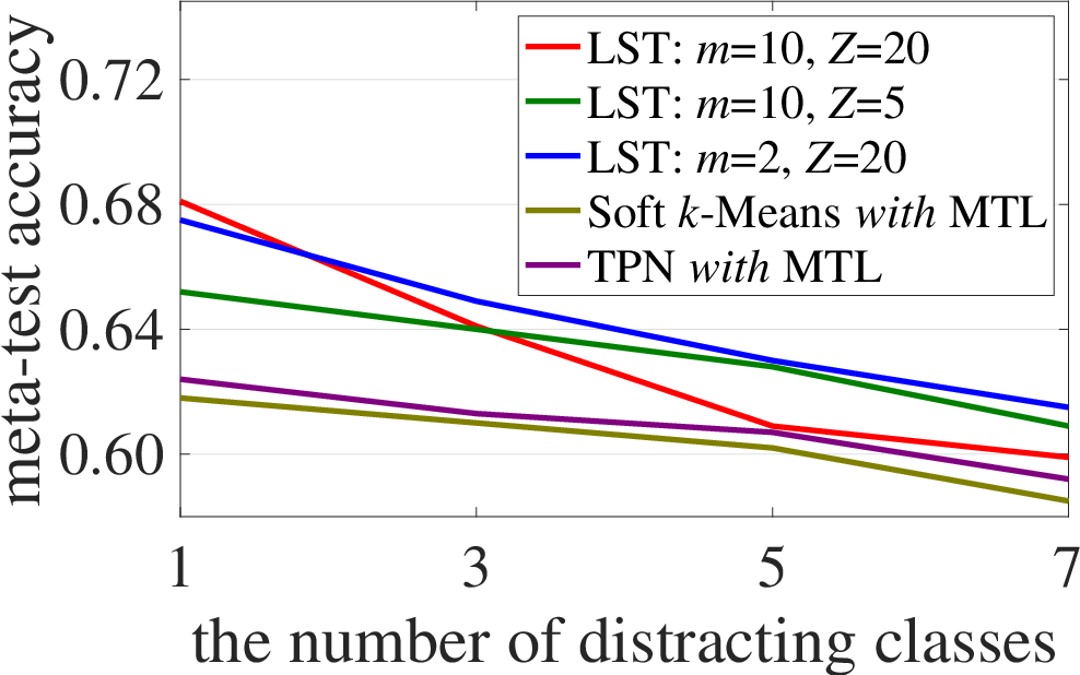
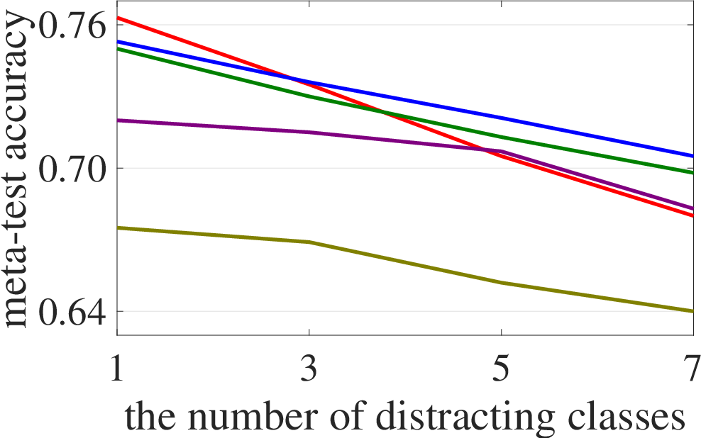
Quantitative analyses on the number of distracting classes. In Figure 4, we show the effects of distracting classes on our LST and related methods (improved versions with MTL) RenICLR2018_semisupervised; TarvainenNIPS17mean_teacher. More distracting classes cause more performance deduction for all methods. Our LST achieves the top performance, especially more than higher than TPN LiuICLR2019transductive in the hardest case with distracting classes. Among our different settings, we can see that LST with less re-training steps, i.e., a smaller value, works better for reducing the effect from a larger number of distracting classes.
(a) (b)
Displaying the performance of pseudo-labeling.. Taking the miniImageNet 1-shot as an example, we record the accuracy of pseudo labeling for meta-training and meta-test (based on our best model recursive, hard, soft), in Table 3 and Table 4, respectively. In meta-training, we can see the accuracy grows from (iter=) to (iter=), and it reaches saturation after iterations. There are recursive stages during meta-test. From stage- to stage-, the average accuracy of meta-test tasks using our best method increases from to .
| Iteration | ||||||||
|---|---|---|---|---|---|---|---|---|
| Accuracy | 47.0 | 64.1 | 65.9 | 70.0 | 71.2 | 70.9 | 71.3 | 71.5 |
| Stage | 1 | 2 | 3 | 4 | 5 | 6 |
|---|---|---|---|---|---|---|
| Accuracy | 59.8 | 63.6 | 65.1 | 66.9 | 67.9 | 68.8 |
Generalization ability. Our LST approach is in principle able to generalize to other optimization-based FSC methods. To validate this, we replace MTL with a classical method called MAML FinnAL17. We implement the experiments of MAML-based LST (using recursive,hard,soft) and compare with the same 4CONV-arch model TPN LiuICLR2019transductive. On miniImagenet -shot, our method gets the accuracy of ( for w/), outperforming TPN by ( for w/). On the more challenging dataset tieredImageNet (1-shot) we achieve even higher superiority, i.e., ( for w/).
6 Conclusions
We propose a novel LST approach for semi-supervised few-shot classification. A novel recursive-learning-based self-training strategy is proposed for robust convergence of the inner loop, while a cherry-picking network is meta-learned to select and label the unsupervised data optimized in the outer loop. Our method is general in the sense that any optimization-based few-shot method with different base-learner architectures can be employed. On two popular few-shot benchmarks, we found consistent improvements over both state-of-the-art FSC and SSFSC methods.
Acknowledgments
This research is part of NExT research which is supported by the National Research Foundation, Prime Minister’s Office, Singapore under its IRC@SG Funding Initiative. It is also partially supported by German Research Foundation (DFG CRC 1223), and National Natural Science Foundation of China (61772359, 61671289, 61771301, 61521062).
References
- (1) Antreas Antoniou, Harrison Edwards, and Amos Storkey. How to train your maml. In ICLR, 2019.
- (2) Lee Dong-Hyun. Pseudo-label: The simple and efficient semi-supervised learning method for deep neural networks. In ICML Workshops, 2013.
- (3) Chelsea Finn, Pieter Abbeel, and Sergey Levine. Model-agnostic meta-learning for fast adaptation of deep networks. In ICML, 2017.
- (4) Chelsea Finn, Kelvin Xu, and Sergey Levine. Probabilistic model-agnostic meta-learning. In NeurIPS, 2018.
- (5) Luca Franceschi, Paolo Frasconi, Saverio Salzo, Riccardo Grazzi, and Massimiliano Pontil. Bilevel programming for hyperparameter optimization and meta-learning. In ICML, 2018.
- (6) Yves Grandvalet and Yoshua Bengio. Semi-supervised learning by entropy minimization. In NIPS, 2004.
- (7) Erin Grant, Chelsea Finn, Sergey Levine, Trevor Darrell, and Thomas L. Griffiths. Recasting gradient-based meta-learning as hierarchical bayes. In ICLR, 2018.
- (8) Kaiming He, Xiangyu Zhang, Shaoqing Ren, and Jian Sun. Deep residual learning for image recognition. In CVPR, 2016.
- (9) Samuli Laine and Timo Aila. Temporal ensembling for semi-supervised learning. In ICLR, 2017.
- (10) Kwonjoon Lee, Subhransu Maji, Avinash Ravichandran, and Stefano Soatto. Meta-learning with differentiable convex optimization. In CVPR, 2019.
- (11) Yoonho Lee and Seungjin Choi. Gradient-based meta-learning with learned layerwise metric and subspace. In ICML, 2018.
- (12) Fei-Fei Li, Robert Fergus, and Pietro Perona. One-shot learning of object categories. IEEE Trans. Pattern Anal. Mach. Intell., 28(4):594–611, 2006.
- (13) Akshay Mehrotra and Ambedkar Dukkipati. Generative adversarial residual pairwise networks for one shot learning. arXiv, 1703.08033, 2017.
- (14) Nikhil Mishra, Mostafa Rohaninejad, Xi Chen, and Pieter Abbeel. Snail: A simple neural attentive meta-learner. In ICLR, 2018.
- (15) Takeru Miyato, Andrew M. Dai, and Ian J. Goodfellow. Virtual adversarial training for semi-supervised text classification. arXiv, 1605.07725, 2016.
- (16) Tsendsuren Munkhdalai and Hong Yu. Meta networks. In ICML, 2017.
- (17) Tsendsuren Munkhdalai, Xingdi Yuan, Soroush Mehri, and Adam Trischler. Rapid adaptation with conditionally shifted neurons. In ICML, 2018.
- (18) Avital Oliver, Augustus Odena, Colin A. Raffel, Ekin Dogus Cubuk, and Ian J. Goodfellow. Realistic evaluation of deep semi-supervised learning algorithms. In NeurIPS, 2018.
- (19) Chapelle Olivier, Schölkopf Bernhard, and Zien Alexander. Semi-supervised learning, volume ISBN 978-0-262-03358-9. Cambridge, Mass.: MIT Press, 2006.
- (20) Boris N. Oreshkin, Pau Rodríguez, and Alexandre Lacoste. TADAM: task dependent adaptive metric for improved few-shot learning. In NeurIPS, 2018.
- (21) Sachin Ravi and Hugo Larochelle. Optimization as a model for few-shot learning. In ICLR, 2017.
- (22) Mengye Ren, Eleni Triantafillou, Sachin Ravi, Jake Snell, Kevin Swersky, Joshua B. Tenenbaum, Hugo Larochelle, and Richard S. Zemel. Meta-learning for semi-supervised few-shot classification. In ICLR, 2018.
- (23) Marcus Rohrbach, Sandra Ebert, and Bernt Schiele. Transfer learning in a transductive setting. In NIPS, 2013.
- (24) Olga Russakovsky, Jia Deng, Hao Su, Jonathan Krause, Sanjeev Satheesh, Sean Ma, Zhiheng Huang, Andrej Karpathy, Aditya Khosla, Michael Bernstein, Alexander C. Berg, and Li Fei-Fei. ImageNet Large Scale Visual Recognition Challenge. International Journal of Computer Vision, 115(3):211–252, 2015.
- (25) Andrei A. Rusu, Dushyant Rao, Jakub Sygnowski, Oriol Vinyals, Razvan Pascanu, Simon Osindero, and Raia Hadsell. Meta-learning with latent embedding optimization. In ICLR, 2019.
- (26) Adam Santoro, Sergey Bartunov, Matthew Botvinick, Daan Wierstra, and Timothy P. Lillicrap. Meta-learning with memory-augmented neural networks. In ICML, 2016.
- (27) Eli Schwartz, Leonid Karlinsky, Joseph Shtok, Sivan Harary, Mattias Marder, Rogério Schmidt Feris, Abhishek Kumar, Raja Giryes, and Alexander M. Bronstein. Delta-encoder: an effective sample synthesis method for few-shot object recognition. In NeurIPS, 2018.
- (28) Evan Shelhamer, Jonathan Long, and Trevor Darrell. Fully convolutional networks for semantic segmentation. IEEE Trans. Pattern Anal. Mach. Intell., 39(4):640–651, 2017.
- (29) Jake Snell, Kevin Swersky, and Richard S. Zemel. Prototypical networks for few-shot learning. In NIPS, 2017.
- (30) Qianru Sun, Yaoyao Liu, Tat-Seng Chua, and Bernt Schiele. Meta-transfer learning for few-shot learning. In CVPR, 2019.
- (31) Flood Sung, Yongxin Yang, Li Zhang, Tao Xiang, Philip H. S. Torr, and Timothy M. Hospedales. Learning to compare: Relation network for few-shot learning. In CVPR, 2018.
- (32) Antti Tarvainen and Harri Valpola. Mean teachers are better role models: Weight-averaged consistency targets improve semi-supervised deep learning results. In NIPS, 2017.
- (33) Isaac Triguero, Salvador García, and Francisco Herrera. Self-labeled techniques for semi-supervised learning: taxonomy, software and empirical study. Knowl. Inf. Syst., 42(2):245–284, 2015.
- (34) Oriol Vinyals, Charles Blundell, Tim Lillicrap, Koray Kavukcuoglu, and Daan Wierstra. Matching networks for one shot learning. In NIPS, 2016.
- (35) Yu-Xiong Wang, Ross B. Girshick, Martial Hebert, and Bharath Hariharan. Low-shot learning from imaginary data. In CVPR, 2018.
- (36) Yongqin Xian, Saurabh Sharma, Bernt Schiele, and Zeynep Akata. f-VAEGAN-D2: A feature generating framework for any-shot learning. In CVPR, 2019.
- (37) Liu Yanbin, Juho Lee, Minseop Park, Saehoon Kim, and Yi Yang. Transductive propagation network for few-shot learning. In ICLR, 2019.
- (38) LeCun Yann, Bengio Yoshua, and Hinton Geoffrey. Deep learning. Nature, 521(7553):436, 2015.
- (39) David Yarowsky. Unsupervised word sense disambiguation rivaling supervised methods. In ACL, 1995.
- (40) Chiyuan Zhang, Samy Bengio, Moritz Hardt, Benjamin Recht, and Oriol Vinyals. Understanding deep learning requires rethinking generalization. In ICLR, 2017.
- (41) Ruixiang Zhang, Tong Che, Zoubin Grahahramani, Yoshua Bengio, and Yangqiu Song. Metagan: An adversarial approach to few-shot learning. In NeurIPS, 2018.
Supplementary materials
These supplementary materials include the additional results of using different numbers of stages in the recursive training in our LST method (recursive, hard, soft) (§A), the supplementary results (on the tieredImageNet dataset) of Figure 3 in the main paper (§B), and the comparable results using a very limited number of unlabeled data, i.e. unlabeled samples per class (§C). There are also experimental results about when our LST method is equiped with different backbones (§D).
A Using different numbers of recursive stages
During meta-validation, we test our method using different numbers of recursive stages, and show the results in Figure 5. We observe that the performance of our method is saturated when running after e.g. stages. In experiments, we split samples (per class) as the unlabeled dataset. At each recursive stage, we sample a subset, i.e. for 1-shot and for 5-shot. After a few stages, the model has sampled and learned all unlabeled samples, therefore, its performance gets saturated. We choose the peak values, so we use stages for 1-shot and for 5-shot during meta-test, on both miniImageNet and tieredImageNet.


(a) (b)
B Using different numbers of re-training steps
In Figure 6, we report the results on tieredImageNet 1-shot, using different numbers of re-training steps, as the supplementary of Figure 3 in the main paper. The same as in Figure 3, each curve shows the results obtained at the final recursive stage. Corresponding methods are (a) our LST, (b) our ablative method (no meta) with off-the-shelf MTL model [30], and (c) the (no meta) that directly uses pre-trained ResNet-12 model [30]. We can observe that very few re-training steps, i.e. steps, are enough for our LST model to converge to the best performance, similar to the conclusion drawn from the results on miniImageNet.


(a) (b) (c)
C Using a small number of unlabeled samples
We also consider using limited number of unlabeled samples ( per class) in the experiments. In this setting, we evaluate our LST method (the version without recursive due to few unlabeled data) as well as related methods, Masked Soft -Means and TPN. Note that same with Table 2 in the main paper, these related methods are equipped with MTL, i.e. using pre-trained ResNet- as backbone, and using more efficient meta operations (scaling and shifting) in the feature extraction part. As shown in Table 5, our method achieves the best performance compared to other two methods, on both benchmarks.
| mini | tiered | mini w/ | tiered w/ | |||||||||
| 1(shot) | 5 | 1 | 5 | 1 | 5 | 1 | 5 | |||||
| hard, soft (Ours w/o recursive) | 61.9 | 75.3 | 72.1 | 82.4 | 60.3 | 75.0 | 70.7 | 82.0 | ||||
| Masked Soft k-Means [22] with MTL | 58.2 | 71.9 | 65.3 | 79.8 | 56.8 | 71.1 | 63.6 | 79.2 | ||||
| TPN [37] with MTL | 59.3 | 71.9 | 67.4 | 80.7 | 58.7 | 70.6 | 67.2 | 80.5 | ||||
D Generalization ability
We incorporate the 4CONV arch. of MAML [3] and the recent FSC method LEO [25] into our LST, respectively. The results are shown in Table 6. For example, on tieredImageNet 1-shot, LST-MAML-4CONV outperforms TPN-4CONV [37] by and (). LST-LEO-ResNet12 outperforms TPN-ResNet12 by and ().
| MAML [3] | LEO [25] | ||||
|---|---|---|---|---|---|
| mini(1-shot) / D | tiered / D | mini / D | tiered / D | ||
| recursive,hard,soft | 54.8 / 52.0 | 58.6 / 55.5 | 66.0 / 63.5 | 75.9 / 74.3 | |
| TPN [37] | 52.8 / 50.4 | 55.7 / 53.5 | 62.7 / 61.3 | 72.1 / 71.5 | |