More than the sum of its parts:
combining parameterized tests of extreme gravity
Abstract
We connect two formalisms that describe deformations away from general relativity, one valid in the strong-field regime of neutrons stars and another valid in the radiative regime of gravitational waves: the post-Tolman-Oppenheimer-Volkoff and the parametrized-post-Einsteinian formalisms respectively. We find that post-Tolman-Oppenheimer-Volkoff deformations of the exterior metric of an isolated neutron star induce deformations in the orbital binding energy of a neutron star binary. Such a modification to the binding energy then percolates into the gravitational waves emitted by such a binary, with the leading-order post-Tolman-Oppenheimer-Volkoff modifications introducing a second post-Newtonian order correction to the gravitational wave phase. The lack of support in gravitational wave data for general relativity deformations at this post-Newtonian order can then be used to place constraints on the post-Tolman-Oppenheimer-Volkoff parameters. As an application, we use the binary neutron star merger event GW170817 to place the constraint (at 90% credibility) on a combination of post-Tolman-Oppenheimer-Volkoff parameters. We also explore the implications of this result to the possible deformations of the mass-radius relation of neutron stars allowed within this formalism. This work opens the path towards theory-independent tests of gravity, combining astronomical observations of neutron stars and gravitational wave observations.
I Introduction
Neutron stars are one of the prime objects in nature for confronting our understanding of fundamental physical interactions against observations Watts et al. 2016; Berti et al. 2015; Doneva and Pappas 2018. Their small size (radius around km) and large mass ( M⊙) result in densities at their core that can exceed that of nuclear saturation density, at which hadronic matter can transmute into exotic forms, by 10 orders of magnitude Lattimer and Prakash 2007. Neutron stars are also extreme gravity objects, second only to black holes in the strength of their gravitational potential and spacetime curvature, with fields that exceed those that we experience in the neighborhood of our Solar System by 9 orders of magnitude. The strong-field regime of neutron stars, critical in determining their structure and stability Oppenheimer and Volkoff 1939; Tolman 1939; Bonolis 2017, demands the use of relativistic gravity to describe these stars, with Einstein’s general relativity (GR) as our canonical theory for doing so. Moreover, neutron stars unlike black holes, allow us to probe how matter couples with the very fabric of spacetime in the strong-field regime Delsate and Steinhoff 2012.
The piercing power of neutron stars as tools to test our understanding of nature is amplified when they are found in binaries. From the discovery of the very first binary pulsar Hulse and Taylor 1975 and the confirmation that its orbital period decays in agreement with GR predictions, through the emission of gravitational waves Damour 2015, to the spectacular detection of the first binary neutron star merger event GW170817 Abbott et al. 2017 by the LIGO/Virgo collaboration (LVC), neutron star binaries have been in the forefront of experimental gravity in astronomical settings with implications to cosmology included Yunes and Siemens 2013; Sakstein and Jain 2017; Baker et al. 2017; Ezquiaga and Zumalacárregui 2017; Creminelli and Vernizzi 2017
Experimental tests of relativistic gravity have a long history Will 1993; Will 2014 and can basically be carried out in two ways. In the first approach, one assumes a particular theory, whose predictions are worked out and then tested against observations. In the second approach, one introduces deformations to the predictions or solutions of GR, in a particular regime of the theory, and one then works out the observational consequences of these deformations to confront them against observations. Both approaches have been successful in aiding our understanding of the nature of gravity. An example of the first approach is the ruling out of Nordström’s theory of gravity (a predecessor to GR), which for example fails to predict the deflection of light by the Sun Dyson et al. 1920; Mehra 1974; Will 2015. An example of the second approach is the parametrized post-Newtonian framework (ppN) Will 1971; Will and Nordtvedt 1972; Nordtvedt and Will 1972, which allowed us to test GR against a myriad of new Solar System tests starting in the 1960s, although early ideas date back to Eddington Eddington 1963.
Can we combine parametrized tests of gravity that involve observations of the strong-field gravity created by isolated neutron stars with those that involve the radiative and dynamical fields generated in the coalescence of neutron star binaries? The purpose of this paper is to build a bridge between two parametrizations for tests of GR: the parametrized post-Tolman-Oppenheimer-Volkoff (post-TOV) formalism Glampedakis et al. 2015; Glampedakis et al. 2016 (which parametrizes deviations to the stellar structure of isolated neutrons stars) and the parametrized-post-Einsteinian (ppE) formalism Yunes and Pretorius 2009; Yunes et al. 2016 (which parametrizes deviations to GR in the inspiral, merger and ringdown of compact binary coalescence). This bridge provides a theory-independent framework to combine constraints on deviations to GR from the observation of the bulk properties of neutron stars and from the generation and propagation of gravitational waves produced in the coalescence of binary neutron stars.
The connection between both formalisms is only possible by realizing that the modified exterior spacetime of neutron stars in the post-TOV formalisms affects the binding energy of a neutron star binary Glampedakis et al. 2016, and thus, the gravitational waves that such a binary emits Yunes and Pretorius 2009. This modification to the binding energy or the gravitational waves emitted can be mapped onto the ppE framework, which we have extended here to encompass a wider set of modifications to the conservative sector of the binary’s Hamiltonian. This allows a particular combination of post-TOV parameters [defined in Eq. (6)] to be mapped to the ppE modification to the gravitational wave Fourier phase [cf. Eqs. (24) and (29)]. We find that modifies the gravitational wave evolution at second post-Newtonian order (2PN)11 1 The PN formalism is one in which the field equations are solved perturbatively as an expansion in weak fields and small velocities. A term of PN order is of relative to the leading-order term, with the orbital speed and the speed of light Blanchet 2014.
The lack of support in gravitational wave data for a GR deformation then allows for constraints on deformations of the exterior metric of isolated neutron stars. In particular, the constraints on GR modifications obtained by the LVC Abbott et al. 2018a for the binary-neutron star gravitational wave event GW170817 Abbott et al. 2018b can be used to place the first observational constraint on , namely at 90% credibility (see Fig. 1). This result strengthens the case for compact binary mergers as laboratories to test GR, something which would otherwise be very hard (if not impossible) with only mass and radius measurements of isolated neutron stars due to strong degeneracies between matter and strong-field gravity. We provide explicit examples of this degeneracy by computing the post-TOV deformations to the mass-radius curves within for a fixed equation of state.
The remainder of the paper presents the details that led to the results summarized above and it is organized as follows. In Sec. I we briefly overview the post-TOV and ppE formalisms, establishing the connection between the two. Next, in Sec. III we use the public data on tests of GR with GW170817 released by LVC to place constraints on a combination of post-TOV parameters. In Sec. IV we discuss the allowed deformation on the mass-radius curves of neutron stars under this constraint, discussing in detail the degeneracies between matter and strong gravity. In Sec. V, we present our conclusions and outline some directions for which our work can be extended. Throughout this work we use geometric units and use a mostly plus metric signature.
II From Post-TOV to ppE
Let us start by briefly reviewing the post-TOV formalism developed in Refs. Glampedakis et al. 2015; Glampedakis et al. 2016 and the ppE formalism introduced in Ref. Yunes and Pretorius 2009 and expanded in Chatziioannou et al. 2012.
II.1 Overview of the post-TOV formalism
The idea behind the post-TOV formalism is quite simple. The formalism is based on the observation that the structure of static, spherically symmetric stars in GR is determined by only two differential equations:
| (1a) | ||||
| (1b) | ||||
which respectively govern the pressure and mass gradients within the star. Here, is the circumferential radius, the mass function, the pressure and the total energy density. The latter two variables are assumed to be related through a barotropic equation of state (EOS), i.e. . For later convenience we recall that can be written as , where is the baryonic rest-mass density and the internal energy per unit baryonic mass.
The post-TOV formalism augments these equations to the form
| (2a) | ||||
| (2b) | ||||
where the first set of post-TOV corrections is
| (3a) | ||||
| (3b) | ||||
and the second set is
| (4a) | ||||
where , and are all dimensionless constants.
The first set (, ) arises from the ppN stellar structure equations Wagoner and Malone 1974; Shapiro and Lightman 1976; Ciufolini and Ruffini 1983; Glampedakis et al. 2015. These non-GR terms in the post-Newtonian regime were then added to the full GR equations to capture effects of modifications to GR. Indeed, the parameters are all related to the usual ppN parameters via , , and . Solar System constraints impose , yielding and in Eq. (2), and thus, we will here only study the second set of post-TOV corrections.
The second set (, ) represents 2PN corrections which can be written in terms of fluid and metric variables. As explained in detail in Ref. Glampedakis et al. 2015, the 2PN terms which can be constructed from these primitive quantities can be gathered in five “families,” each with an infinite number of terms and with each family yielding a distinctive change to the mass-radius relation of neutron stars. Fortunately, 2PN terms belonging to each family exhibit qualitatively the same radial profiles inside a star. This translates into terms belonging to the same family affecting the mass-radius relations in a self-similar manner (cf. Glampedakis et al. 2015, Figs. 3, 6 and 7). This fact allows one to choose a single representative member from each family to be included to the TOV equations. The criteria used in Glampedakis et al. 2015 to make this choice was that of overall magnitude of the modification (relative to other terms in the same family) and simplicity of the analytic form of the term.
Equation (2) is sufficient to determine the interior of the star and its bulk properties i.e. the (Schwarzschild) enclosed mass and the radius [location at which when integrating the post-TOV equation outwards from .]. In Glampedakis et al. 2016, the exterior problem was addressed and it was found that the post-TOV equations result in a post-Schwarzschild exterior metric given by
| (5a) | ||||
| (5b) | ||||
where
| (6) |
is a combination of the post-TOV parameters and
| (7) |
is the Arnowitz-Misner-Deser mass of the star. Equation (7) was obtained under the restriction that , outside of which the calculation of requires solving a transcendental equation and for which the exterior metric cannot be written analytically in the simpler form (5).
The fact that is not unusual in modified theories of gravity (see e.g. Damour and Esposito-Farése 1993). In theories beyond GR, contributions to the star’s mass due to the presence of new degrees of freedom, such as scalar or vector fields arise, although this is not always the case Cisterna et al. 2015; Maselli et al. 2016; Cisterna et al. 2016. We stress that it is , not , which would be observationally inferred, e.g. by using Kepler’s law.
In dynamical situations, such as in the motion of a neutron star binary, these additional degrees of freedom can be excited, and thus, they can open new radiative channels for the system to lose energy, modifying the binary’s dynamic. As formulated, the post-TOV formalism cannot account for the presence of extra fields and hence the radiative loses of the binary will be the same as in GR. On the other hand, since the exterior spacetime is different from that of Schwarzschild, the conservative sector of the binary motion will be different.
As we will see next, the ppE formalism aims to capture generic deviations from GR to both sectors. This will allow us to obtain a mapping between the parameters (that control these deviations) in both formalisms.
II.2 Overwiew of the ppE formalism
The ppE formalism was developed to capture generic deviations from GR in the gravitational waves emitted by a binary system Yunes and Pretorius 2009. These deviations can be separated into those that affect the conservative sector (e.g. the binding energy of the orbit) and the dissipative sector (e.g. the flux of energy). In previous work, the conservative sector was modified in a rather cavalier way, making some assumptions about the structure of the deformations. Let us then here relax some of these assumptions and rederive the modifications.
We begin with the Hamiltonian for a two-body system in the center of mass frame, working to leading order in the post-Newtonian approximation and to leading order in the GR deformation:
| (8) |
where is the relative separation of the binary, is the reduced mass, with the component masses and the total mass, and and are the generalized momenta conjugate to the radial and azimuthal coordinates.
The functions characterize the deformation to the standard Newtonian Hamiltonian. For the purposes of this work, we will parametrize these deformations as
| (9) |
where control the magnitude of the deformation (assumed small here), while control the character of the deformation. We will also here assume that , meaning that all deformations enter at the same post-Newtonian order, and we will discuss later how to relax this assumption. Physically, we can think of as modifying the , and components of the metric respectively. Notice also that if , then the radius and the angle are not your usual circumferential radius and azimuthal angle (though they are related to them via a coordinate transformation).
With this at hand, we can now derive the constants of the motion and the field equations. Assuming the Hamilton equations hold, there are two constants of the motion associated with time translation and azimuthal-angle translation invariance. The former is simply the Hamiltonian itself, which for a binary is the binding energy . The latter is the angular momentum of the orbit, which we can define as . The azimuthal component of the generalized momenta can be obtained from
| (10) |
which then leads to
| (11) |
where have used the definition , and because was assumed to be independent of by Eq. (9).
With this at hand, we can now derive the radial equation of motion in reduced order form. We begin by evaluating , which by Hamilton’s equation is simply , where again we have used that was assumed to be independent of from Eq. (9). We can then rewrite Eq. (II.2) as
Note that , which is associated with a deformation of the -component of the metric does not affect the location in phase space where (or equivalently where ).
Before we can find what the binding energy of the orbit is as a function of the orbital angular frequency, we must determine what the energy and the angular momentum of a circular orbit in this perturbed spacetime is. We can do so by setting and and solving for and , which yields
| (13) | ||||
From the above expression for , we can solve for as well as (i.e. the modification to Kepler’s third law) to find
| (15) |
Using this in Eq. (13), we then find the final expression
| (16) |
Reference Chatziioannou et al. 2012 carried out a similar calculation, except that in their calculation, the whole Newtonian effective potential was modified by the same term, namely
| (17) |
Such a modification lead to a binding energy of the form Chatziioannou et al. 2012
| (18) |
From this, Ref. Chatziioannou et al. 2012 showed that the gravitational waves emitted by a binary, assuming the dissipative sector is not modified (i.e the flux of energy is the same as that in GR), and assuming gravitational waves contain the same two polarizations as in GR, lead to a Fourier detector response (in the stationary phase approximation) of the form
| (19) |
where is the Fourier amplitude and is the Fourier phase. The latter can be decomposed into , where is the Fourier phase in GR, while the GR deformation is
| (20) |
where
| (21) |
and is the gravitational wave frequency.
Given the similarities in the calculations, the easiest way forward is to map the results of Ref. Chatziioannou et al. 2012 to the modifications we are considering here. Comparing the binding energies in Eqs. (18) and (16), we see that
| (22) |
and where we have used that . We then see clearly that the change in the Fourier phase is
| (23) |
This deformation arising from a GR correction to the binding energy can be mapped to the ppE waveform as follows. Noting that the ppE phase is Yunes et al. 2016
| (24) |
we then realize that
| (25a) | ||||
| (25b) | ||||
Therefore, a ppE constraint on for a given value of given a gravitational wave observation that is consistent with GR can be straightforwardly mapped to a constraint on given a value of .
II.3 Relating the parameters in both formalisms
Several paths are possible to relate the post-TOV and the ppE formalisms. The path we choose here is to compare the binding energy and angular momentum of a binary system composed of neutron stars whose metrics in isolation would take the form of Eq. (5). This can be achieved by transforming from the two-body problem to an effective one-body problem, in which a test particle of mass moves in a background of mass . Let us then consider the geodesic motion of a test particle in a generic (but still stationary and spherically symmetric) background.
Consider the line element
| (26) |
where the metric functions and are decomposed as and , and where is a small bookkeeping parameter. In Appendix A we present a detailed analysis of geodesic circular motion in such a perturbed metric, and we compute the change to the binding energy and the angular momentum of the orbit. Identifying , , substituting these expressions into Eqs. (49) and (50), and expanding both in and in , we find
| (27) | ||||
| (28) |
where is a post-TOV parameter.
We can now compare Eq. (27) to Eq. (13) and Eq. (28) to (II.2) to find what , and are in the post-TOV formalism. Doing so, we find that , and . In fact, we could have predicted that had to vanish, because the radial coordinate in the post-TOV formalism is the circumferential radius. With this in hand, the ppE parameters are then simply
| (29) |
This is one of the main results of this paper, since a constraint on can now straightforwardly be mapped to a constraint on and vice versa. Note that one could also use the mapping between to compute the modification to Kepler’s third law through Eq. (15) or the binding energy as a function of the orbital frequency through Eq. (16), but this is not needed here.
In the limit the evolution of a neutron star binary in GR and in the post-TOV formalism become identical. However, we emphasize that this limit does not necessarily correspond to the limit in which the post-TOV equation reduces to the usual GR TOV equations. Indeed, only places a constraint on the combination of some of the post-TOV parameters. Therefore, one can have the situation in which a neutron star binary inspiral is identical to GR, yet the structure of the individual stars is different from GR either because and/or because the nonzero post-TOV parameters are the ones which do not affect the exterior space. Thus, we will refer to the case as the coincident limit.
III Constraints on the post-TOV parameters from GW170817
The LVC released constraints on model-independent deviations from GR to examine the consistency of the GW170817 event with GR predictions Abbott et al. 2018a; LIGO Scientific Collaboration and Virgo Collaboration 2018. The constraints were obtained using a variant of IMRPhenomPv2 Ajith et al. 2007; Ajith et al. 2011; Santamaria et al. 2010; Husa et al. 2016, which improves upon IMRPhenomD Husa et al. 2016; Khan et al. 2016 by phenomenologically including some aspects of spin precession and tidal effects Dietrich et al. 2017; Dietrich et al. 2019. In this variant, deviations from GR are described through relative shifts in the GR PN coefficients of the Fourier phase of IMRPhenomPv2
| (30) |
where are additional free parameters in the model.
The parametrization used by LVC is an implementation of the ppE formalism as explained in Yunes et al. 2016, with and being related as
| (31) |
where is the GR coefficient of the Fourier phase at 2PN order (cf. Appendix B in Khan et al. 2016). Comparing Eqs. (29) and (31) we obtain
| (32) |
which establishes the relation between with .
We can now translate the posterior distribution of into one for by using the MCMC samples available in LIGO Scientific Collaboration and Virgo Collaboration 2018, where, for each step, we calculate the corresponding value of using Eq. (32). The resulting probability density is shown in Fig. 1 with the 90% credible region corresponding to
| (33) |
This is the first constraint on (a combination of) post-TOV parameters and another one of the main results of this paper.
The fact that the posterior of has a peak outside of zero (the coincident limit) is perplexing at first sight and may be misinterpreted as evidence for a deviation from GR, but this is not to be the case. Rather, it reflects the qualitative behavior of the posterior distribution of (see Fig. 1 in Abbott et al. 2018a), which also does not exhibit a peak at and it is skewed to positive values. Both distributions, however, clearly do have a significant amount of support at zero, and thus, they do not indicate an inconsistency with GR. The skewness in the posterior for probably results from the marginalization process over the various parameters that describe the model, the degeneracies between these parameters, and the nonstationarity of the noise in the detectors.
The similarity between the posteriors for and can be understood from the following argument. The two posteriors, and , are related by . The Jacobian of the transformation () can be calculated from Eq. (32), where is independent of . From the MCMC samples we find that the mean value of the prefactor is and thus . Moreover, , which streches relative to . We then come to the conclusion that is nothing but a rescaled version (by the same scale factor) in height and width of . In fact, this simple argument results in a posterior for that is very similar to that shown in Fig. 1.
Having obtained a constraint on , is it possible to translate it into constraints on the three-dimensional parameter space spanned by , and ? The first step to do this, is to fix the prior ranges for these parameters. We take (for the reasons discussed in Sec. II.1) and assume and are in the ranges . The latter domains are chosen such as to include the GR limit and to be large enough to include moderately large values of and to encompass the upper bound . We then draw samples from the probability density function (shown in Fig. 1), and given a value , we then draw samples of , and until Eq. (6) is satisfied.
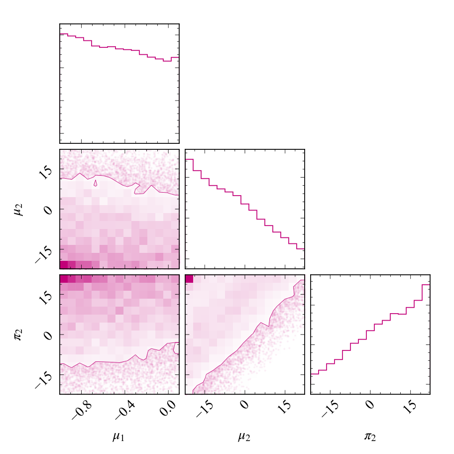
Figure 2 shows the result of this calculation. The diagonal panels in this corner plot show the marginalized posteriors on , and , while the off-diagonal panels show two-dimensional joint posteriors with the 90% credible contours delimited by the solid lines. The constraint on leaves essentially unconstrained, while the favored values for and are set by the bound of our priors. This occurs due to the strong degeneracy between these parameters arising from Eq. (6), which, together with Eq. (33), constrains . Thus, if the prior ranges of and were extended, the marginalized posteriors in Fig. 2 would retain their qualitative shapes, with peaks at the edge of their priors, as has an infinite number of solutions.
IV Degeneracies between matter and gravity models
In the previous section we have constrained the magnitude of the post-TOV parameter , as well as , and . How do these results impact the allowed deformations away from a GR mass-radius curve as allowed by the post-TOV formalism? Could one, for example, use these deformed mass-radius regions, together with observations of the mass and radius of isolated neutron stars, to place further constraints on post-TOV parameters? We will show in this section explicitly that this is not possible due to degeneracies between post-TOV deformations and the EOS.
To answer this question, we construct mass-radius curves with a restricted set of post-TOV equations and a fixed set of representative EOSs. The set of post-TOV equations is obtained from Eq. (2) by fixing all parameters to zero other than , and , and we make this choice because these three parameters are the only ones that can be directly probed by electromagnetic or gravitational wave phenomena. The set of EOSs consists of the SLy Douchin and Haensel 2001 and APRb Akmal et al. 1998 EOSs, which are favored by the tidal deformability measurements of the constituents of GW170817 Abbott et al. 2018c in GR and the observation of two solar masses neutron stars Demorest et al. 2010; Antoniadis et al. 2013; Cromartie et al. 2019. With this set of post-TOV equations and EOSs, we then construct one thousand mass-radius curves each with a different choice of post-TOV parameters that lay within the bound of Eq. (33). The value of these parameters was selected as follows. First, we drew random samples from the probability distribution function , only accepting values that satisfy (33). Next, we drew samples of , and (as in Sec. III) until Eq. (6) is met.
The results of these integrations are shown in Fig. 3 for EOS APRb; the results for EOS SLy being very similar, so we do not show them here. In this figure, the vertical hatched (yellow) region contains all the mass-radius curves that are consistent with the post-TOV constraints derived in this paper, all truncated at the the maximum mass of the (stable) sequence. As is evident, the post-TOV formalism is capable of capturing a wide variety of curves that span a large region of the mass-radius plane, including exotic types, which e.g. have very low maximum masses M⊙(despite both EOSs supporting M⊙ stars in GR). Other curves can enter the region in the mass-radius plane that is excluded in GR (the “causality” curve), which is derived by requiring only a very minimal set of assumptions on the underlying unknown EOS Rhoades and Ruffini 1974; Kalogera and Baym 1996, with some even extending close to Buchdahl’s limit.22 2 This high-compactness stars are supported in the post-TOV formalism due to the fact that the modification can be associated to pressure anisotropy, with the difference between radial and tangential pressures being [see Eq. (4)]. Pressure anisotropy has have long been known to support ultracompact stars Bowers and Liang 1974. Further exotica include mass-radius curves that do not have an extrema at . These generically allow for very large radii ( km), even when the mass is M⊙ . More common curves are only small deformations away from the GR result.
Although the region of the mass-radius plane allowed by Eq. (33) alone is rather large, it can be reduced by combining other sources of information on the masses and radii of neutron stars. For instance, by imposing that the mass-radius curves are consistent with (i) the existence of neutron stars with masses M⊙ Cromartie et al. 2019 and (ii) the canonical radius bound km Kumar and Landry 2019, then 99.3% (for SLy) and 96.3% (for APRb) of the curves investigated are excluded. The resulting tighter contour due to the surviving mass-radius curves is shown by the horizontally hatched (red) regions in Fig. 3.
Figure 4 vividly shows several difficulties in testing extreme gravity with observations of isolated neutron stars that yield mass and radius measurements alone. First, even in GR, our ignorance on the underlying neutron star EOS gives riseto mass-radius curves that can overlap (see the intersection of the SLy and APRb curves in Fig. 4). Second, even in the event of the EOS being tightly constrained in the future (under the assumption of neutron stars are described by GR), a measurement of still leads to degeneracies between the post-TOV parameters , and , as shown in the previous section Each value of should correspond to a specific theory of gravity, and this degeneracy prevents us from singling one out. Third, the fact that the contours in Fig. 4 change as we change the EOS makes the degeneracy between EOS and theory of gravity explicit. This degeneracy arises in the post-TOV formalism in a very explicit way: the post-TOV equations (with ) can be mapped into an effective barotropic EOS, with and Glampedakis et al. 2015. Therefore, observations of isolated neutron stars that yield mass and radius measurements alone cannot really be used to test gravity, unless more information is contained in the data, which can be folded into the models to test GR.
V Conclusions and outlook
Neutron star observations, both through electromagnetic and gravitational-wave astronomy, offer us a unique look into the fundamental interactions of nature. For gravity (in particular) it allows us to probe both the strong-field regime of neutron star interiors and the radiative aspects of gravity, when these object are found in binary systems. To be able to do theory-independent tests of gravity through neutron star observations, we have combined the post-TOV and ppE formalisms, constructing a single, unified framework for which tests of gravity can be performed from the radiative level down to the level of stellar structure.
This framework is particularly relevant in light of ongoing events on the observational front. For instance, the Neutron Star Interior Composition Explorer (NICER) mission Gendreau et al. 2012; Arzoumanian et al. 2014; Gendreau and Arzoumanian 2017 will soon release the mass and radius measurements of a number of neutron stars within 10% precision and probes the effects of spacetime curvature on the motion of photons. Moreover, LIGO/Virgo is currently on its third scientific observing run, with a binary neutron star merger candidate already observed and tens of events expected to be seen in the next years. It would be interesting to combine these upcoming observational results to further explore the resulting constraints on the post-TOV parameters and thereby constrain modifications to GR in a theory-independent way.
For instance, the contours in Fig. 4 reveal that the largest variability occurs for massive stars with M⊙. One of NICER’s targets (PSR J1614–2230) has a mass of 1.93 M⊙ Fonseca et al. 2016; Miller 2016 and a radius measurement of it would constrain this region of the mass-radius plane. In turn, these constraints could also be used to probe deviations from GR in a number of astrophysical scenarios, for instance in the quasiperiodic oscillations on matter disks in accreting neutron stars Glampedakis et al. 2016, or in the pulse profiles emitted by hot spots on the surface of rotating neutron stars (complementary to constraints on scalar-tensor gravity Silva and Yunes 2019). We have here only taken a first step on using this new framework and hope to explore further its applications in the near future.
Acknowledgments
We thank the post-TOV practitioners Emanuele Berti, Kostas Glampedakis and George Pappas for numerous discussions on the topic over the years. We also thank Alejandro Cárdenas-Avendaño, Katerina Chatziioannou, Remya Nair, Thomas Sotiriou and Jacob Stanton for discussions on different aspects related to this work. Finally, we thank the anonymous referee for carefully reading our work. This work was supported by NASA Grants No. NNX16AB98G and No. 80NSSC17M0041. N. Y. also acknowledges the hospitality of KITP where some of this work was completed.
Appendix A Derivation of the binding energy
In this Appendix, we derive general formulas for the changes to the energy and angular momentum of point particles orbiting in the static, spherically symmetric spacetime of an object of mass .
A.1 Particle motion in perturbed spacetimes
Consider the line element
| (34) |
in Schwarzschild coordinates, on which a massive particle follows geodesic motion, with trajectory , where is the proper time. Let be the particle’s four-velocity, constrained by
As usual, the spacetime symmetries imply the existence of two Killing vector fields which result in two conserved quantities
| (35) |
respectively, the energy and angular momentum (per unit mass) of the particle.
Due to the conserved angular momentum, orbits are confined to a single plane, which we take, without loss of generality to be the one for which . Using this result we find that
| (36) |
Let us consider spacetimes with metric g, which are a small deformations to a static, spherically symmetric background . More specifically, let us write the metric functions and as
| (37) |
where (in this Appendix only) denotes a small bookkeeping parameter. For convenience, we omit hereafter the dependence on of the functions introduced above. Using these decompositions of and , into Eq. (36) and then solving for , we find to leading order in ,
Equation () suggests the definition of a zeroth-order effective potential ,
| (39) |
and a leading-order correction ,
| (40) |
such that Eq. () becomes
| (41) |
A.2 Properties of particles in circular orbits
Now let us focus on the properties of particles in (not necessarily stable) circular orbits that we denote by . These orbits satisfy the conditions
| (42) |
where .
As a warm-up exercise, let us consider the limit and obtain general formulas of the (zeroth-order) energy and angular momentum of particles in circular orbits on . This calculation is particularly simple, because can be easily isolated from the equation. With a little algebra we can obtain the general formulas
| (43) | ||||
| (44) |
In the particular limit of the Schwarzschild spacetime () we readily obtain the familiar results
| (45) |
Now, let us consider the general problem and obtain the corrections to and due to the perturbation in Eq. (). To do this, we first solve Eq. (42) for and . Next, we expand the resulting expressions to leading order in . The outcome of this exercise is that and can be written as
| (46) |
where the corrections to the zeroth-order energy and angular momentum [cf. Eqs. (43) and (44)] are
| (47) |
and
| (48) |
These expressions are the main result of this Appendix. Notice the absence of in these expressions.
Finally, we can solve for and and write
| (49) | ||||
| (50) |
our final results.
Appendix B Orbital period decay rate
In this appendix we derive an expression for the orbital period rate of change in the post-TOV formalism following closely Sampson et al. 2013 and obtain an order-of-magnitude bound on from binary systems.
We start by assuming that energy is carried away from a circular binary according to the GR gravitational-wave luminosity formula
| (51) |
at the expense of the orbital binding energy given by (16), i.e. .
Taking a time-derivative of Eq. (16) and using we find:
| (52) |
Now, let us return to (51). We can eliminate in favor of by using the modified Kepler’s law (15). Solving for , expanding in , and then substituting the resulting expression in Eq. (51) gives
| (53) |
We can now use Eqs. (52) and (53) in the energy balance law, solve for (while expanding once more in , ) and find:
| (54) |
which is the main result of this appendix, where
| (55) |
is the corresponding GR result. In the particular case of the post-TOV metric, we find after using , and that
| (56) |
A simple constraint on (independent from the one in the main text) can thus be obtained as follows. Since binary pulsar observations of are in remarkable agreement with GR up to some observational error we can write . Therefore, the post-TOV correction in Eq. (56) is bound by , which then constrains to be
| (57) |
where is characteristic velocity of the system and (for the quasicircular system PSR J0737-3039 Yunes and Hughes 2010), giving the weak bound . This result is seven orders of magnitude weaker than the bound obtained from GW170817 and exemplifies the constraining power of gravitational wave events on modifications to GR relative to binary pulsar constraints33 3 At first sight our upper bounds on are outside the perturbative regime () used to derive our main formulas. These expansions are only formal. The true small parameter bound to be is the combination, e.g. (similarly for the other parameters) which does remain small during the inspiral..
References
- Watts et al. (2016) A. L. Watts et al., Rev. Mod. Phys. 88, 021001 (2016), arXiv:1602.01081 [astro-ph.HE] .
- Berti et al. (2015) E. Berti et al., Class. Quant. Grav. 32, 243001 (2015), arXiv:1501.07274 [gr-qc] .
- Doneva and Pappas (2018) D. D. Doneva and G. Pappas, Astrophys. Space Sci. Libr. 457, 737 (2018), arXiv:1709.08046 [gr-qc] .
- Lattimer and Prakash (2007) J. M. Lattimer and M. Prakash, Phys. Rept. 442, 109 (2007), arXiv:astro-ph/0612440 [astro-ph] .
- Oppenheimer and Volkoff (1939) J. R. Oppenheimer and G. M. Volkoff, Phys. Rev. 55, 374 (1939).
- Tolman (1939) R. C. Tolman, Phys. Rev. 55, 364 (1939).
- Bonolis (2017) L. Bonolis, European Physical Journal H 42 (2017), 10.1140/epjh/e2017-80014-4, arXiv:1703.09991 [physics.hist-ph] .
- Delsate and Steinhoff (2012) T. Delsate and J. Steinhoff, Phys. Rev. Lett. 109, 021101 (2012), arXiv:1201.4989 [gr-qc] .
- Hulse and Taylor (1975) R. A. Hulse and J. H. Taylor, Astrophys. J. 195, L51 (1975).
- Damour (2015) T. Damour, Class. Quant. Grav. 32, 124009 (2015), arXiv:1411.3930 [gr-qc] .
- Abbott et al. (2017) B. P. Abbott et al. (LIGO Scientific, Virgo), Phys. Rev. Lett. 119, 161101 (2017), arXiv:1710.05832 [gr-qc] .
- Yunes and Siemens (2013) N. Yunes and X. Siemens, Living Rev. Rel. 16, 9 (2013), arXiv:1304.3473 [gr-qc] .
- Sakstein and Jain (2017) J. Sakstein and B. Jain, Phys. Rev. Lett. 119, 251303 (2017), arXiv:1710.05893 [astro-ph.CO] .
- Baker et al. (2017) T. Baker, E. Bellini, P. G. Ferreira, M. Lagos, J. Noller, and I. Sawicki, Phys. Rev. Lett. 119, 251301 (2017), arXiv:1710.06394 [astro-ph.CO] .
- Ezquiaga and Zumalacárregui (2017) J. M. Ezquiaga and M. Zumalacárregui, Phys. Rev. Lett. 119, 251304 (2017), arXiv:1710.05901 [astro-ph.CO] .
- Creminelli and Vernizzi (2017) P. Creminelli and F. Vernizzi, Phys. Rev. Lett. 119, 251302 (2017), arXiv:1710.05877 [astro-ph.CO] .
- Will (1993) C. M. Will, Theory and experiment in gravitational physics (1993).
- Will (2014) C. M. Will, Living Rev. Rel. 17, 4 (2014), arXiv:1403.7377 [gr-qc] .
- Dyson et al. (1920) F. W. Dyson, A. S. Eddington, and C. Davidson, Phil. Trans. Roy. Soc. Lond. A220, 291 (1920).
- Mehra (1974) J. Mehra, Einstein, Hilbert, and the theory of gravitation (1974).
- Will (2015) C. M. Will, Class. Quant. Grav. 32, 124001 (2015), arXiv:1409.7812 [physics.hist-ph] .
- Will (1971) C. M. Will, Astrophys. J. 163, 611 (1971).
- Will and Nordtvedt (1972) C. M. Will and K. Nordtvedt, Jr., Astrophys. J. 177, 757 (1972).
- Nordtvedt and Will (1972) K. J. Nordtvedt and C. M. Will, Astrophys. J. 177, 775 (1972).
- Eddington (1963) A. S. Eddington, The mathematical theory of relativity (1963).
- Glampedakis et al. (2015) K. Glampedakis, G. Pappas, H. O. Silva, and E. Berti, Phys. Rev. D92, 024056 (2015), arXiv:1504.02455 [gr-qc] .
- Glampedakis et al. (2016) K. Glampedakis, G. Pappas, H. O. Silva, and E. Berti, Phys. Rev. D94, 044030 (2016), arXiv:1606.05106 [gr-qc] .
- Yunes and Pretorius (2009) N. Yunes and F. Pretorius, Phys. Rev. D80, 122003 (2009), arXiv:0909.3328 [gr-qc] .
- Yunes et al. (2016) N. Yunes, K. Yagi, and F. Pretorius, Phys. Rev. D94, 084002 (2016), arXiv:1603.08955 [gr-qc] .
- Abbott et al. (2018a) B. P. Abbott et al. (LIGO Scientific, Virgo), (2018a), arXiv:1811.00364 [gr-qc] .
- Blanchet (2014) L. Blanchet, Living Rev. Rel. 17, 2 (2014), arXiv:1310.1528 [gr-qc] .
- Abbott et al. (2018b) B. P. Abbott et al. (LIGO Scientific, Virgo), (2018b), arXiv:1811.12907 [astro-ph.HE] .
- Chatziioannou et al. (2012) K. Chatziioannou, N. Yunes, and N. Cornish, Phys. Rev. D86, 022004 (2012), [Erratum: Phys. Rev.D95,no.12,129901(2017)], arXiv:1204.2585 [gr-qc] .
- Wagoner and Malone (1974) R. V. Wagoner and R. C. Malone, ApJ 189, L75 (1974).
- Shapiro and Lightman (1976) S. T. Shapiro and A. P. Lightman, ApJ 207, 263 (1976).
- Ciufolini and Ruffini (1983) I. Ciufolini and R. Ruffini, ApJ 275, 867 (1983).
- Damour and Esposito-Farése (1993) T. Damour and G. Esposito-Farése, Phys. Rev. Lett. 70, 2220 (1993).
- Cisterna et al. (2015) A. Cisterna, T. Delsate, and M. Rinaldi, Phys. Rev. D92, 044050 (2015), arXiv:1504.05189 [gr-qc] .
- Maselli et al. (2016) A. Maselli, H. O. Silva, M. Minamitsuji, and E. Berti, Phys. Rev. D93, 124056 (2016), arXiv:1603.04876 [gr-qc] .
- Cisterna et al. (2016) A. Cisterna, T. Delsate, L. Ducobu, and M. Rinaldi, Phys. Rev. D93, 084046 (2016), arXiv:1602.06939 [gr-qc] .
- LIGO Scientific Collaboration and Virgo Collaboration (2018) LIGO Scientific Collaboration and Virgo Collaboration, “LIGO Document P1800115-v12,” (2018), [Online; accessed 21-May-2019].
- Ajith et al. (2007) P. Ajith et al., Gravitational wave data analysis. Proceedings: 11th Workshop, GWDAW-11, Potsdam, Germany, Dec 18-21, 2006, Class. Quant. Grav. 24, S689 (2007), arXiv:0704.3764 [gr-qc] .
- Ajith et al. (2011) P. Ajith et al., Phys. Rev. Lett. 106, 241101 (2011), arXiv:0909.2867 [gr-qc] .
- Santamaria et al. (2010) L. Santamaria et al., Phys. Rev. D82, 064016 (2010), arXiv:1005.3306 [gr-qc] .
- Husa et al. (2016) S. Husa, S. Khan, M. Hannam, M. Pürrer, F. Ohme, X. Jiménez Forteza, and A. Bohé, Phys. Rev. D93, 044006 (2016), arXiv:1508.07250 [gr-qc] .
- Khan et al. (2016) S. Khan, S. Husa, M. Hannam, F. Ohme, M. Pürrer, X. Jiménez Forteza, and A. Bohé, Phys. Rev. D93, 044007 (2016), arXiv:1508.07253 [gr-qc] .
- Dietrich et al. (2017) T. Dietrich, S. Bernuzzi, and W. Tichy, Phys. Rev. D96, 121501 (2017), arXiv:1706.02969 [gr-qc] .
- Dietrich et al. (2019) T. Dietrich et al., Phys. Rev. D99, 024029 (2019), arXiv:1804.02235 [gr-qc] .
- Douchin and Haensel (2001) F. Douchin and P. Haensel, Astron. Astrophys. 380, 151 (2001), arXiv:astro-ph/0111092 [astro-ph] .
- Akmal et al. (1998) A. Akmal, V. R. Pandharipande, and D. G. Ravenhall, Phys. Rev. C58, 1804 (1998), arXiv:nucl-th/9804027 [nucl-th] .
- Abbott et al. (2018c) B. P. Abbott et al. (LIGO Scientific, Virgo), Phys. Rev. Lett. 121, 161101 (2018c), arXiv:1805.11581 [gr-qc] .
- Demorest et al. (2010) P. Demorest, T. Pennucci, S. Ransom, M. Roberts, and J. Hessels, Nature 467, 1081 (2010), arXiv:1010.5788 [astro-ph.HE] .
- Antoniadis et al. (2013) J. Antoniadis et al., Science 340, 6131 (2013), arXiv:1304.6875 [astro-ph.HE] .
- Cromartie et al. (2019) H. T. Cromartie et al., (2019), arXiv:1904.06759 [astro-ph.HE] .
- Kumar and Landry (2019) B. Kumar and P. Landry, (2019), arXiv:1902.04557 [gr-qc] .
- Rhoades and Ruffini (1974) C. E. Rhoades, Jr. and R. Ruffini, Phys. Rev. Lett. 32, 324 (1974).
- Kalogera and Baym (1996) V. Kalogera and G. Baym, Astrophys. J. 470, L61 (1996), arXiv:astro-ph/9608059 [astro-ph] .
- Alsing et al. (2018) J. Alsing, H. O. Silva, and E. Berti, Mon. Not. Roy. Astron. Soc. 478, 1377 (2018), arXiv:1709.07889 [astro-ph.HE] .
- Bowers and Liang (1974) R. L. Bowers and E. P. T. Liang, ApJ 188, 657 (1974).
- Gendreau et al. (2012) K. C. Gendreau, Z. Arzoumanian, and T. Okajima, in Space Telescopes and Instrumentation 2012: Ultraviolet to Gamma Ray, Proc. SPIE, Vol. 8443 (2012) p. 844313.
- Arzoumanian et al. (2014) Z. Arzoumanian et al., in Space Telescopes and Instrumentation 2014: Ultraviolet to Gamma Ray, Proc. SPIE, Vol. 9144 (2014) p. 914420.
- Gendreau and Arzoumanian (2017) K. Gendreau and Z. Arzoumanian, Nature Astronomy 1, 895 (2017).
- Fonseca et al. (2016) E. Fonseca et al., Astrophys. J. 832, 167 (2016), arXiv:1603.00545 [astro-ph.HE] .
- Miller (2016) M. C. Miller, Astrophys. J. 822, 27 (2016), arXiv:1602.00312 [astro-ph.HE] .
- Silva and Yunes (2019) H. O. Silva and N. Yunes, Class. Quant. Grav. 36, 17LT01 (2019), arXiv:1902.10269 [gr-qc] .
- Sampson et al. (2013) L. Sampson, N. Yunes, and N. Cornish, Phys. Rev. D88, 064056 (2013), [Erratum: Phys. Rev.D88,no.8,089902(2013)], arXiv:1307.8144 [gr-qc] .
- Yunes and Hughes (2010) N. Yunes and S. A. Hughes, Phys. Rev. D82, 082002 (2010), arXiv:1007.1995 [gr-qc] .