RKHSMetaMod: An R package to estimate the Hoeffding decomposition of a complex model by solving RKHS ridge group sparse optimization problemThanks: Halaleh Kamari, Université Paris-Saclay, France, @, Sylvie Huet, INRAE, France, @, Marie-Luce Taupin, Université Evry Val d’Essonne, France, @.
Abstract
In this paper, we propose an R package, called RKHSMetaMod, that implements a procedure for estimating a meta-model of a complex model. The meta-model approximates the Hoeffding decomposition of the complex model and allows us to perform sensitivity analysis on it. It belongs to a reproducing kernel Hilbert space that is constructed as a direct sum of Hilbert spaces. The estimator of the meta-model is the solution of a penalized empirical least-squares minimization with the sum of the Hilbert norm and the empirical -norm. This procedure, called RKHS ridge group sparse, allows both to select and estimate the terms in the Hoeffding decomposition, and therefore, to select and estimate the Sobol indices that are non-zero. The RKHSMetaMod package provides an interface from R statistical computing environment to the C++ libraries Eigen and GSL. In order to speed up the execution time and optimize the storage memory, except for a function that is written in R, all of the functions of this package are written using the efficient C++ libraries through RcppEigen and RcppGSL packages. These functions are then interfaced in the R environment in order to propose a user-friendly package.
Keywords: Meta model, Hoeffding decomposition, Ridge Group Sparse penalty, Reproducing Kernel Hilbert Spaces.
1 Introduction
Consider a phenomenon described by a model depending on input variables . This model from to may be a known model that is calculable in all points of , i.e. , or it may be an unknown regression model defined as follows:
| (1) |
where the error is assumed to be centered with a finite variance, i.e. and . The components of are independent with a known law on , a subset of . The number of components of may be large. The model may present high complexity as strong non-linearities and high order interaction effects, and it is assumed to be square-integrable, i.e. . Based on the data points , we estimate a meta-model that approximates the Hoeffding decomposition of . This meta-model belongs to a reproducing kernel Hilbert space (RKHS), which is constructed as a direct sum of the Hilbert spaces leading to an additive decomposition including variables and interactions between them [\citeauthoryearDurrande, Ginsbourger, Roustant, and CarraroDurrande et al.2013]. The estimator of the meta-model is calculated by minimizing an empirical least-squares criterion penalized by the sum of two penalty terms: the Hilbert norm and the empirical norm [\citeauthoryearHuet and TaupinHuet and Taupin2017]. This procedure allows us to select the subsets of variables that contribute to predict . The estimated meta-model is used to perform sensitivity analysis, and therefore, to determine the influence of each variable and groups of them on the output variable .
In the classical framework of sensitivity analysis, the function is calculable in all points of , and one may use the method of [\citeauthoryearSobolSobol1993] to perform sensitivity analysis on . Let us briefly introduce this method: The independency between the components of leads to write the function according to its Hoeffding decomposition ([\citeauthoryearSobolSobol1993], [\citeauthoryearVan der VaartVan der Vaart1998]):
| (2) |
The terms in this decomposition are defined using the conditional expected values:
These terms are known as the constant term, main effects, interactions of order two and so on. Let be the set of all subsets of with dimension to . For all and , let be the vector with components , . For a set let be its cardinality, and for all , let be the function associated with in Equation (2). Then Equation (2) can be expressed as follows:
| (3) |
This decomposition is unique, all the terms , are centered, and they are orthogonal with respect to . The functions and , in Equation (3) are square-integrable. As any two terms of decomposition (3) are orthogonal, by squaring (3) and integrating it with respect to the distribution of , a decomposition of the variance of is obtained as follows:
| (4) |
The Sobol indices associated with the group of variables , are defined by:
| (5) |
For each , expresses the fraction of variance of explained by . For all , when , the s are referred to as the first order indices; when , i.e. and , they are referred to as the second order indices or the interaction indices of order two (between and ); and the same holds for .
The total number of the Sobol indices to be calculated is equal to , which raises exponentially with the number of the input variables. When is large, the evaluation of all the indices can be computationally demanding and even not reachable.
In practice, only the indices of order not higher than two are calculated.
However, only the first and second order indices may not provide a good information on the model sensitivities. In order to provide better information on the model sensitivities, [\citeauthoryearHomma and SaltelliHomma and
Saltelli1996] proposed to calculate the first order and the total indices defined as follows:
Let be the set of all the subsets of including , then .
For all , denotes the total effect of . It expresses the fraction of variance of explained by alone and all the interactions of it with the other variables.
The total indices allow us to rank the input variables with respect to the amount of their effect on the output variable. However, they do not provide complete information on the model sensitivities as do all the Sobol indices.
The classical computation of the Sobol indices is based on the Monte Carlo methods (see for example: [\citeauthoryearSobolSobol1993] for the main effect and interaction indices, and [\citeauthoryearSaltelliSaltelli2002] for the main effect and total indices). For models that are expensive to evaluate, the Monte Carlo methods lead to a high computational burden. Moreover, in the case where is large, is complex and the calculation of the variances (see Equation (4)) is numerically complicated or not possible (as in the case where the model is unknown) the methods described above are not applicable. Another approach consists in approximating by a simplified model, called a meta-model, which is much faster to evaluate and to perform sensitivity analysis on it. Beside the approximations of the Sobol indices of at a lower computational cost, a meta-model provides a deeper view of the input variables effects on the model output. Among the meta-modelling methods proposed in the literature, the expansion based on polynomial Chaos ([\citeauthoryearWienerWiener1938], [\citeauthoryearSchoutensSchoutens2000]) can be used to approximate the Hoeffding decomposition of [\citeauthoryearSudretSudret2008]. The principle of the polynomial Chaos is to project onto a basis of orthonormal polynomials. The polynomial Chaos expansion of is written as [\citeauthoryearSoize and GhanemSoize and Ghanem2004]:
| (6) |
where are the coefficients, and are the multivariate orthonormal polynomials associated with which are determined according to the distribution of the components of . In practice, expansion (6) shall be truncated for computational purposes, and the model may be approximated by , where is determined using a truncation scheme. The Sobol indices are obtained then by summing up the squares of the suitable coefficients. [\citeauthoryearBlatman and SudretBlatman and Sudret2011] proposed a method for truncating the polynomial Chaos expansion and an algorithm based on the least angle regression for selecting the terms in the expansion. In this approach, according to the distribution of the components of , a unique family of orthonormal polynomials is determined. However, this family may not be necessarily the best functional basis to approximate well.
Gaussian Process (GP) can also be used to construct meta-models as highlighted in [\citeauthoryearWelch, Buck, Sacks, Wynn, Mitchell, and MorrisWelch et al.1992], [\citeauthoryearOakley and O’HaganOakley and O’Hagan2004], [\citeauthoryearKleijnenKleijnen2007, \citeauthoryearKleijnenKleijnen2009], [\citeauthoryearMarrel, Iooss, Laurent, and RoustantMarrel et al.2009], [\citeauthoryearDurrande, Ginsbourger, and RoustantDurrande et al.2012], [\citeauthoryearLe Gratiet, Cannamela, and IoossLe Gratiet et al.2014]. The principle is to consider that the prior knowledge about the function , can be modelled by a GP with a mean and a covariance kernel . To perform sensitivity analysis from a GP model, one may replace the true model with the mean of the conditional GP and deduce the Sobol indices from it. A review on the meta-modelling based on polynomial Chaos and GP is presented in [\citeauthoryearLe Gratiet, Marelli, and SudretLe Gratiet et al.2017].
[\citeauthoryearDurrande, Ginsbourger, Roustant, and CarraroDurrande et al.2013] considered a class of the functional approximation methods similar to the GP and obtained a meta-model that satisfies the properties of the Hoeffding decomposition. They proposed to approximate by functions belonging to a RKHS which is a direct sum of the Hilbert spaces. Their RKHS is constructed in a way that the projection of onto , denoted , is an approximation of the Hoeffding decomposition of . The function is defined as the minimizer over the functions of the criterion
Let be the scalar product in , let also and be the reproducing kernels associated with the RKHS and the RKHS , respectively. The properties of the RKHS insures that any function , is written as the following decomposition:
| (7) |
where is constant, and is defined by . For more details on the RKHS construction and the definition of the Hilbert norm see Section 6.1.1 in 6.1.
For all , the functions are centered and for all , the functions and are orthogonal with respect to . Therefore, the decomposition of the function presented in Equation (7) is its Hoeffding decomposition. As the function belongs to the RKHS , it is decomposed as its Hoeffding decomposition, , and each function approximates the function in Equation (3). The number of terms that should be estimated in the Hoeffding decomposition of is equal to , which may be huge since it rises very quickly by increasing . In order to deal with this problem, in the regression framework, one may estimate by a sparse meta-model . To this end, the estimation of is done on the basis of observations by minimizing a least-squares criterion suitably penalized in order to deal with both the non-parametric nature of the problem and the possibly large number of functions that have to be estimated. In the classical framework of the sensitivity analysis one may calculate a sparse approximation of using least-squares penalized criterion as it is done in the non-parametric regression framework. In order to obtain a sparse solution of a minimization problem, the penalty function should enforce the sparsity. There exists various ways of enforcing sparsity for a minimization (maximization) problem, see for example [\citeauthoryearHastie, Tibshirani, and WainwrightHastie et al.2015] for a review. Some methods, such as the Sparse Additive Models (SpAM) procedure ([\citeauthoryearRavikumar, Lafferty, Liu, and WassermanRavikumar et al.2009], [\citeauthoryearLiu, Wasserman, and LaffertyLiu et al.2009]) are based on a combination of the -norm with the empirical -norm: where is the squared empirical -norm of the univariate function . The Component Selection and Smoothing Operator (COSSO) method developed by [\citeauthoryearLin and ZhangLin and Zhang2006] enforces sparsity using a combination of the -norm with the Hilbert norm: . Instead of focusing on only one penalty term, one may consider a more general family of estimators, called doubly penalized estimator, which is obtained by minimizing a criterion penalized by the sum of two penalty terms. [\citeauthoryearRaskutti, Wainwright, and YuRaskutti et al.2009, \citeauthoryearRaskutti, Wainwright, and YuRaskutti et al.2012] proposed a doubly penalized estimator, which is the solution of the minimization of a least-squares criterion penalized by the sum of a sparsity penalty term and a combination of the -norm with the Hilbert norm:
| (8) |
where are the tuning parameters that should be suitably chosen.
[\citeauthoryearMeier, van de Geer, and BühlmannMeier et al.2009] proposed a related family of estimators, based on the penalization with the empirical -norm. Their penalty function is the sum of the sparsity penalty term, , and a smoothness penalty term. [\citeauthoryearHuet and TaupinHuet and Taupin2017] considered the same approximation functional spaces as [\citeauthoryearDurrande, Ginsbourger, Roustant, and CarraroDurrande et al.2013], and obtained a doubly penalized estimator of a meta-model which approximates the Hoeffding decomposition of . Their estimator is the solution of the least-squares minimization penalized by the penalty function defined in Equation (8) adapted to the multivariate setting,
| (9) |
This procedure, called RKHS ridge group sparse, estimates the groups that are suitable for predicting , and the relationship between and for each group. The obtained estimator, called RKHS meta-model, is used then to estimate the Sobol indices of . This approach renders it possible to estimate the Sobol indices for all groups in the support of the RKHS meta-model, including the interactions of possibly high order, a point known to be difficult in practice.
In this paper, we introduce an R package, called RKHSMetaMod, that implements the RKHS ridge group sparse procedure. The functions of this package allows us to:
- (1)
calculate the reproducing kernels and their associated Gram matrices (see Section 3.1),
- (2)
- (3)
choose the tuning parameters and (see Equation (9)), using a procedure that leads to obtain the best RKHS meta-model in terms of the prediction quality,
- (4)
estimate the Sobol indices of the function (see Section 2.3).
The current version of the package supports uniformly distributed input variables on . However, it could easily be adapted to a different distribution of input variables by making a small modification to one of its functions (see Remark 3 of Section 3.1).
Let us give a brief overview of the related existing statistical packages to RKHSMetaMod. The R package sensitivity is designed to implement sensitivity analysis methods and provides the approaches for numerical calculation of the Sobol indices. In particular, Kriging method can be used to reduce the number of observations in global sensitivity analysis. The function sobolGP of the package sensitivity builds a Kriging based meta-model using the function km of the package DiceKriging [\citeauthoryearRoustant, Ginsbourger, and DevilleRoustant et al.2012], and estimates its Sobol indices. This procedure can also be done using the function km and the function fast99 of the package sensitivity (see Section 4.5. of [\citeauthoryearRoustant, Ginsbourger, and DevilleRoustant et al.2012]). In this case, the idea is once again to build a Kriging based meta-model using the function km and then estimate its Sobol indices using the function fast99. In both cases the true function is substituted by a Kriging based meta-model and then its Sobol indices are estimated. In the sobolGP function, the Sobol indices are estimated by Monte Carlo integration, while the fast99 function estimates them using the extended-FAST method [\citeauthoryearSaltelli, Tarantola, and ChanSaltelli et al.1999]. To reduce the computational burden when dealing with large datasets and complex models, in RKHSMetaMod package, we propose to use the empirical variances to estimate the Sobol indices (see Section 2.3). Besides, the estimation of the Sobol indices in the RKHSMetaMod package is done based on the RKHS meta-model which is a sparse estimator. It is beneficial since instead of calculating the Sobol indices of all groups , only the Sobol indices associated with the groups in the support of the RKHS meta-model are computed (see Section 2.3). Moreover, the functions sobolGP and fast99 provide the estimation of the first order and the total Sobol indices only, while the procedure in the RKHSMetaMod package makes it possible to estimate the high order Sobol indices. The R packages DiceKriging and DiceOptim (Deep Inside Computer Experiments Kriging/Optim) [\citeauthoryearRoustant, Ginsbourger, and DevilleRoustant et al.2012] implement the Kriging based meta-models to estimate complex models in the high dimensional context. They provide different GP (Kriging) models corresponding to the Gaussian, Matérn, Exponential and Power-Exponential correlation functions. The estimation of the parameters of the correlation functions in these packages relies on the global optimizer with gradient genoud algorithm of the package rgenoud [\citeauthoryearMebane and SekhonMebane and Sekhon2011]. These packages do not implement any method of the sensitivity analysis themselves. However, some authors (see Section 4.5. of [\citeauthoryearRoustant, Ginsbourger, and DevilleRoustant et al.2012] for example) perform sensitivity analysis on their estimated meta-models by employing the functions of the package sensitivity. The R package RobustGaSP (Robust Gaussian Stochastic Process) [\citeauthoryearGu, Palomo, and BergerGu et al.2019] approximates a complex model by a GP meta-model. This package implements marginal posterior mode estimation of the GP model parameters. The estimation method in this package insures the robustness of the parameter estimation in the GP model, and allows one also to identify input variables that have no effect on the variability of the function under study. The R package mlegp (maximum likelihood estimates of Gaussian processes) [\citeauthoryearDancik and DormanDancik and Dorman2008] provides functions to implement both meta-modelling approaches and sensitivity analysis methods. It obtains maximum likelihood estimates of GP model for the output of costly computer experiments. The GP models are built either on the basis of the Gaussian correlation function or on the basis of the first degree polynomial trend. The sensitivity analysis methods implemented in this package include Functional Analysis of Variance (FANOVA) decomposition, plot functions to obtain diagnostic plots, main effects, and second order interactions. The prediction quality of the meta-model depends on the quality of the estimation of its parameters and more precisely the estimation of parameters in the correlation functions [\citeauthoryearKennedy and O’HaganKennedy and O’Hagan2000]. The maximum likelihood estimation of these parameters often produce unstable results, and as a consequence, the obtained meta-model may have an inferior prediction quality ([\citeauthoryearGu, Wang, and BergerGu et al.2018], [\citeauthoryearGuGu2019]). The RKHSMetaMod package is devoted to the meta-model estimation on the RKHS . It implements the convex optimization algorithms to calculate meta-models; provides the functions to compute the prediction error of the obtained meta-models; performs the sensitivity analysis on the obtained meta-models and more precisely calculate their Sobol indices. The convex optimization algorithms used in this package are all written using C++ libraries, and are adapted to take into account the problem of high dimensionality in this context. This package is available from the Comprehensive R Archive Network (CRAN) [\citeauthoryearKamariKamari2019].
The organization of the paper is as follows: In the next Section, we describe the estimation method. In Section 3, we present in details the algorithms used in the RKHSMetaMod package to obtain the RKHS meta-model. In Section 6.2, an overview of the package functions as well as a brief documentation of them are given. Section 4 includes two parts: In the first part, Section 4.1, the performance of the RKHSMetaMod package functions is validated through a simulation study. In the second part, Section 4.2, the comparison in terms of the predictive accuracy between the RKHS meta-model and the Kriging based meta-models from RobustGaSP [\citeauthoryearGu, Palomo, and BergerGu et al.2019] and DiceKriging [\citeauthoryearRoustant, Ginsbourger, and DevilleRoustant et al.2012] packages is given through two examples.
2 Estimation method
In this Section, we present: the RKHS ridge group sparse and the RKHS group lasso procedures (see 2.1), the strategy of choosing the tuning parameters in the RKHS ridge group sparse algorithm (see 2.2), and the calculation of the empirical Sobol indices of the RKHS meta-model (see 2.3).
2.1 RKHS ridge group sparse and RKHS group lasso procedures
Let us denote by the number of observations. The dataset consists of a vector of observations , and a matrix of features with components For some tuning parameters , , , the RKHS ridge group sparse criterion is defined by,
| (10) |
where represents the matrix of variables corresponding to the -th group, i.e. and where is the empirical -norm of defined by the sample as
The penalty function in the criterion (10) is the sum of the Hilbert norm and the empirical norm, which allows us to select few terms in the additive decomposition of over sets . Moreover, the Hilbert norm favours the smoothness of the estimated , .
Let be the set of functions.
Then the RKHS meta-model is defined by,
| (11) |
According to the Representer Theorem [\citeauthoryearKimeldorf and WahbaKimeldorf and Wahba1970], the non-parametric functional minimization problem described above is equivalent to a parametric minimization problem. Indeed, the solution of the minimization problem (11) belonging to the RKHS is written as , where for some matrix we have for all ,
| (12) |
Let be the Euclidean norm (called also -norm) in , and for each , let be the Gram matrix associated with the kernel , i.e. . Let also be the matrix that satisfies , and let and be the minimizers of the following penalized least-squares criterion:
Then the estimator defined in Equation (11) satisfies,
Remark 1.
The constraint is crucial for theoretical properties, but the value of is generally unknown and has no practical usefulness. In this package, it is not taken into account in the parametric minimization problem.
For each , let and be the weights that are chosen suitably. We define and with .
Remark 2.
This formulation simplifies the choice of the tuning parameters since instead of tuning parameters and , , only two parameters and are tuned. Moreover, the weights and , may be of interest in practice. For example, one can take weights that increase with the cardinal of in order to favour the effects with small interaction order between variables.
For the sake of simplicity, in the rest of this paper for all the weights and are assumed to be set as one, and the RKHS ridge group sparse criterion is then expressed as follows:
| (13) |
If we consider only the second part of the penalty function in the criterion (13) ( i.e. set ), we obtain the RKHS group lasso criterion as follows:
| (14) |
which is a group lasso criterion [\citeauthoryearYuan and LinYuan and Lin2006] up to a scale transformation.
In the RKHSMetaMod package, the RKHS ridge group sparse algorithm is initialized using the solutions obtained by solving the RKHS group lasso algorithm. Indeed, the penalty function in the RKHS group lasso criterion (14) insures the sparsity in the solution. Therefore, for a given value of , by implementing the RKHS group lasso algorithm (see Section 3.2.1), a RKHS meta-model with few terms in its additive decomposition is obtained. The support and the coefficients of a RKHS meta-model which is obtained by implementing RKHS group lasso algorithm will be denoted by and , respectively. From now on the tuning parameter in the RKHS group lasso criterion will be denoted by:
| (15) |
2.2 Choice of the tuning parameters
While dealing with an optimization problem of a criterion of the form (13), one of the essential steps is to choose appropriately the tuning parameters. Cross-validation is generally used for that purpose. Nevertheless in the context of high-dimensional complex models, the computational time for a cross-validation procedure may be prohibitively high. Therefore we propose a procedure based on a single testing data set:
- •
we first choose, a grid of values of the tuning parameters and ;
Let be the smallest value of (see Equation (15)), such that the solution to the minimization of the RKHS group lasso problem for all is . We have,(16) In order to set up the grid of values of , one may find and then a grid of values of could be defined by for The grid of values of is chosen by the user.
- •
next, for the grid of values of and , we calculate a sequence of estimators. Each estimator associated with the pair in the grid of values of and , denoted by , is the solution of the RKHS ridge group sparse optimization problem or the RKHS group lasso optimization problem if .
- •
finally, the obtained estimators are evaluated using a testing dataset, The prediction error associated with the estimator is calculated by,
where for being the support of the estimator we have,
The pair with the smallest value of the prediction error is chosen, and the estimator is considered as the best estimator of the function , in terms of the prediction error.
In the RKHSMetaMod package, the algorithm to calculate a sequence of the RKHS meta-models, the value of , and the prediction error are implemented as RKHSMetMod, mumax, and PredErr functions, respectively. These functions are described in Section 6.2, and illustrated in Example 1, Example 2, and Examples 1, 2, 3, respectively.
2.3 Estimation of the Sobol indices
The variance of the function is estimated by the variance of the estimator . As the estimator belongs to the RKHS , it admits the Hoeffding decomposition and,
In order to reduce the computational cost in practice, one may estimate the variances of , by their empirical variances. Let be the empirical mean of , , then:
For the groups that do not belong to the support of , we have and for the groups that belong to the support of , the estimators of the Sobol indices of are defined by,
In the RKHSMetaMod package, the algorithm to calculate the empirical Sobol indices , is implemented as SIemp function. This function is described in Section 6.2.2 and illustrated in Examples 1, 2, 3.
3 Algorithms
The RKHSMetaMod package implements two optimization algorithms: the RKHS ridge group sparse (see Algorithm 2) and the RKHS group lasso (see Algorithm 1). These algorithms rely on the Gram matrices , that have to be positive definite. Therefore, the first and essential step in this package is to calculate these matrices and insure their positive definiteness. This step is detailed in an algorithm that is described in the next Section. The second step is to estimate the RKHS meta-model. In the RKHSMetaMod package, two different objectives based on different procedures are considered to calculate this estimator:
- 1.
The RKHS meta-model with the best prediction quality.
The procedure to calculate the RKHS meta-model with the best prediction quality has been described in Section 2.2: a sequence of values of the tuning parameters is considered, and the RKHS meta-models associated with each pair of the values of are calculated. For , the RKHS meta-model is obtained by solving the RKHS group lasso optimization problem, while for the RKHS ridge group sparse optimization problem is solved to calculate the RKHS meta-model. The obtained RKHS meta-models are evaluated by considering a new dataset and the RKHS meta-model with the minimum value of the prediction error is chosen as the best estimator.
- 2.
The RKHS meta-model with at most groups in its support, i.e. .
First, the tuning parameter is set as zero. Then, a value of for which the number of groups in the solution of the RKHS group lasso optimization problem is equal to , is computed. This value of will be denoted by . Finally, the RKHS meta-models containing at most groups in their support are obtained by implementing the RKHS ridge group sparse algorithm for a grid of values of and . This procedure is described in more details in Section 3.2.3.
3.1 Calculation of the Gram matrices
The available kernels in the RKHSMetaMod package are: Gaussian kernel, Matérn kernel, Brownian kernel, quadratic kernel and linear kernel. The usual presentation of these kernels is given in Table 1.
| Kernel type | Mathematics formula for | RKHSMetaMod name |
|---|---|---|
| Gaussian | "gaussian" | |
| Matérn 3/2 | "matern" | |
| Brownian | "brownian" | |
| Quadratic | "quad" | |
| Linear | "linear" |
The choice of the kernel that is done by the user determines the functional approximation space. For a chosen kernel, the algorithm to calculate the Gram matrices , in the RKHSMetaMod package, is implemented as calcKv function. This algorithm is based on three essential points:
- (1)
Modify the chosen kernel:
In order to satisfy the conditions of constructing the RKHS described in Section 6.1.1, these kernels are modified according to Equation (19). Let us take the example of the Brownian kernel:
The RKHS associated with the Brownian kernel is well known to be with the inner product Easy calculations lead to obtain the Brownian kernel as follows,The RKHS associated with the kernel is the set , and we have
Remark 3.
In the current version of the package, we consider the input variables that are uniformly distributed on . In order to consider the input variables that are not distributed uniformly, it suffices to modify a part of the function calcKv related to the calculation of the kernels , . For example, for being distributed with law on , the kernel associated with the Brownian kernel is calculated as follows,
The other parts of the function calcKv remain unchanged.
- (2)
Calculate the Gram matrices for all :
First, for all , the Gram matrices associated with kernels are calculated using Equation (19), Then, for all , the Gram matrices associated with kernel are computed by - (3)
Insure the positive definiteness of the matrices :
The output of the function calcKv is one of the input arguments of the functions associated with the RKHS group lasso and the RKHS ridge group sparse algorithms. Throughout these algorithms we need to calculate the inverse and the square root of the matrices . In order to avoid the numerical problems and insure the invertibility of the matrices , it is mandatory to have these matrices positive definite. One way to render the matrices positive definite is to add a nugget effect to them. That is, to modify matrices by adding a diagonal with a constant term, i.e. . The value of epsilon is computed based on the data and through a part of the algorithm of the function calckv. Let us briefly explain this part of the algorithm:
For each group , let be the eigenvalues associated with the matrix . Set and . For some fixed value of tolerance "tol", and for each matrix , if : then, the eigenvalues of are replaced by , with "epsilon" being equal to "tol". The value of "tol" is set as by default, but one may consider a smaller or a greater value for it depending on the kernel chosen and the value of .
The function calcKv is described in Section 6.2.2 and illustrated in Example 2.
3.2 Optimization algorithms
The RKHS meta-model is the solution of one of the optimization problems: the minimization of the RKHS group lasso criterion presented in Equation (14) (if ), or the minimization of the RKHS ridge group sparse criterion presented in Equation (13) (if ). In the following, the algorithms to solve these optimization problems are presented.
3.2.1 RKHS group lasso
A popular technique for doing group wise variable selection is group lasso. With this procedure, depending on the value of the tuning parameter , an entire group of predictors may drop out of the model. An efficient algorithm for solving group lasso problem is the classical block coordinate descent algorithm ([\citeauthoryearBoyd, Parikh, Chu, Peleato, and EcksteinBoyd et al.2011], [\citeauthoryearBubeckBubeck2015]). Following the idea of [\citeauthoryearFuFu1998], [\citeauthoryearYuan and LinYuan and Lin2006] implemented a block wise descent algorithm for the group lasso penalized least-squares under the condition that the model matrices in each group are orthonormal. A block coordinate (gradient) descent algorithm for solving the group lasso penalized logistic regression is then developed by [\citeauthoryearMeier, van de Geer, and BühlmannMeier et al.2008]. This algorithm is implemented in the R package grplasso available from CRAN [\citeauthoryearMeierMeier2020]. [\citeauthoryearYang and ZouYang and Zou2015] proposed a unified algorithm named group wise majorization descent for solving the general group lasso learning problems by assuming that the loss function satisfies a quadratic majorization condition. The implementation of their work is done in the gglasso R package available from CRAN [\citeauthoryearYang, Zou, and BhatnagarYang et al.2020].
In order to solve the RKHS group lasso optimization problem, we use the classical block coordinate descent algorithm. The minimization of criterion (see Equation (14)) is done along each group at a time. At each step of the algorithm, the criterion is minimized as a function of the current block’s parameters, while the parameters values for the other blocks are fixed to their current values. The procedure is repeated until convergence. This procedure leads to Algorithm 1 (see 6.1 for more details on this procedure).
3.2.2 RKHS ridge group sparse
In order to solve the RKHS ridge group sparse optimization problem, we propose an adapted block coordinate descent algorithm. This algorithm is provided in two steps:
- Step
Initialize the input parameters by the solutions of the RKHS group lasso algorithm for each value of the tuning parameter , and implement the RKHS ridge group sparse algorithm through the active support of the RKHS group lasso solutions until it achieves convergence. This step is provided in order to decrease the execution time. In fact, instead of implementing the RKHS ridge group sparse algorithm over the set of all groups , it is implemented only over the groups in the support of the solution of the RKHS group lasso algorithm, .
- Step
This procedure leads to Algorithm 2 (see 6.1 for more details on this procedure).
3.2.3 RKHS meta-model with at most groups in its support
By considering some prior information about the data, one may be interested in a RKHS meta-model with the number of groups in its support not greater than some "". In order to obtain such an estimator, we provide the following procedure in the RKHSMetaMod package:
- •
First, the tuning parameter is set as zero and a value of for which the solution of the RKHS group lasso algorithm, Algorithm 1, contains exactly groups in its support is computed. This value is denoted by .
- •
Then, the RKHS ridge group sparse algorithm, Algorithm 2, is implemented by setting the tuning parameter equal to and a grid of values of the tuning parameter .
This procedure leads to Algorithm 3.
This algorithm is implemented in the RKHSMetaMod package, as function RKHSMetModqmax (see Section "Main RKHSMetaMod functions" (supplementary materials) for more details on this function).
Remark 4.
As both terms in the penalty function of criterion (13) enforce sparsity to the solution, the estimator obtained by solving the RKHS ridge group sparse associated with the pair of the tuning parameters may contain a smaller number of groups than the solution of the RKHS group lasso optimization problem (i.e. the RKHS ridge group sparse with ). And therefore, the estimated RKHS meta-model contains at most "" groups in its support.
4 RKHSMetaMod through examples
4.1 Simulation study
Let us consider the g-function of Sobol [\citeauthoryearSaltelli, Chan, and ScottSaltelli et al.2009] in the Gaussian regression framework, i.e. . The error term is a centered Gaussian random variable with variance , and the function is the g-function of Sobol defined over by,
| (17) |
The Sobol indices of the g-function can be expressed analytically:
Set , , and . With these values of coefficients , the variables and explain of the variance of the function (see Table 4).
In this Section, three examples are presented. In all examples, the value of Dmax is set as three. Example 1 illustrates the use of the RKHSMetMod function by considering three different kernels, "matern", "brownian", and "gaussian" (see Table 1), and three datasets of observations and input variables. The larger datasets with observations and input variables are studied in Examples 2 and 3.
In each example, two independent datasets are generated: to estimate the meta-models, and to estimate the prediction errors. The design matrices and are the Latin Hypercube Samples of the input variables that are generated using maximinLHS function of the package lhs available at CRAN [\citeauthoryearCarnellCarnell2021]:
R> library(lhs); X <- maximinLHS(n, d); XT <- maximinLHS(n, d)
The response variables and are calculated as and , where , and are centered Gaussian random variables with :
R> a <- c(0.2, 0.6, 0.8, 100, 100, 100, 100, 100, 100, 100)[1:d]
R> g=1; for (i in 1:d) g = g*(abs(4*X[,i]-2)+a[i])/(1+a[i])
R> sigma <- 0.2
R> epsilon <- rnorm(n, 0, sigma*sigma); Y <- g + epsilon
R> gT=1; for (i in 1:d) gT = gT*(abs(4*XT[,i]-2)+a[i])/(1+a[i])
R> epsilonT <- rnorm(n, 0, sigma*sigma); YT <- gT + epsilonT
Example 1.
RKHS meta-model estimation using RKHSMetMod function:
In this example, three datasets of points maximinLHS over are generated with and , and a grid of five values for each of the tuning parameters and is considered as follows:
For each dataset, the experiment is repeated times.
At each repetition, the RKHS meta-models associated with the pair of the tuning parameters are estimated using the RKHSMetMod function:
R> Dmax <- 3; kernel <- "matern" # kernel <- "brownian" # kernel <- "gaussian"
R> gamma <- c(0.2, 0.1, 0.01, 0.005, 0); frc <- c(4,8,16,32,64)
R> res <- RKHSMetMod(Y, X, kernel, Dmax, gamma, frc, FALSE)
These meta-models are evaluated using a testing dataset. The prediction errors are computed for them using the PredErr function. The RKHS meta-model with minimum prediction error is chosen to be the best estimator for the model. Finally, the Sobol indices are computed for the best RKHS meta-model using the function SIemp:
R> Err <- PredErr(X, XT, YT, mu, gamma, res, kernel, Dmax)
R> SI <- SI_emp(res, Err)
The vector "mu" is the values of the tuning parameter that are calculated throughout the function RKHSMetMod (see argument "frc" in Table 12). It could be recovered from the output of the RKHSMetMod function as follows:
R> mu <- vector()
R> l <- length(gamma); for(i in 1:length(frc))mu[i] <- res[[(i-1)*l+1]]$mu
The performances of this method for estimating a meta-model are evaluated by considering a third dataset , , with . The global prediction error is calculated as follows:
Let be the best RKHS meta-model obtained in the repetition , , then
The values of obtained for different kernels and values of are given in Table 2.
As expected the value of decreases as increases. The lowest values of are obtained when using the "matern" kernel.
In order to sum up the behaviour of the procedure for estimating the Sobol indices, we consider the mean square error (MSE) criterion obtained by , where for each group , denotes the true values of the Sobol indices, and is the empirical Sobol indices of the best RKHS meta-model in repetition .
The obtained values of MSE for different kernels and values of are given in Table 3.
As expected, the values of MSE are smaller for larger values of . The smallest values are obtained when using "matern" kernel.
The means of the empirical Sobol indices of the best RKHS meta-models through all repetitions for and "matern" kernel are displayed in Table 4.
| sum | ||||||||
|---|---|---|---|---|---|---|---|---|
| 43.30 | 24.30 | 19.20 | 5.63 | 4.45 | 2.50 | 0.57 | 99.98 | |
| 46.10 | 26.33 | 20.62 | 2.99 | 2.22 | 1.13 | 0.0 | 99.39 |
It appears that the estimated Sobol indices are close to the true ones, nevertheless, they are overestimated for the main effects, i.e. groups , and underestimated for the interactions of order two and three, i.e. groups .
Note that the strategy of choosing the tuning parameters is based on the minimization of the prediction error of the estimated meta-model, which may not minimize the error of estimating the Sobol indices.
Taking into account the results obtained for this Example 1, the calculations in the rest of the examples is done using only the "matern" kernel.
Example 2.
A time-efficient strategy to obtain the "optimal" tuning parameters when dealing with large data sets:
A dataset of points maximinLHS over with and is generated. First, we use functions calcKv and mumax to compute the eigenvalues and eigenvectors of the positive definite matrices , and the value of , respectively:
R> kernel <- "matern"; Dmax <- 3
R> Kv <- calc_Kv(X, kernel, Dmax, TRUE, TRUE)
R> mumax <- mu_max(Y, Kv$kv)
Then, we consider the two following steps:
- 1.
Set and, Calculate the RKHS meta-models associated with the values of by using the function RKHSgrplasso. Gather the obtained RKHS meta-models in a list, "resg" (while this job could be done with the function RKHSMetMod by setting , in this example, we use the function RKHSgrplasso in order to avoid the re-calculation of ’s at the next step). Thereafter, for each estimator in resg, the prediction error is calculated by considering a new dataset and using the function PredErr. The value of with the smallest error of prediction in this step is denoted by . Let us implement this step:
For a grid of values of , a sequence of the RKHS meta-models are calculated and gathered in the "resg" list:
R> frc <- c(4,8,16,32,64,128,256,512,1024)
R> mug <- mumax/frc
R> resg <- list();resg <- list()
R> for(i in 1:length(mug))
R> resg[[i]] <- RKHSgrplasso(Y,Kv, mug[i],1000,FALSE)
R> resg[[i]] <- list("mug"=mug,"gamma"=0,"MetaModel"=resg[[i]])
R>
Output resg contains nine RKHS meta-models and they are evaluated using a testing dataset:
R> gamma <- c(0); Errg <- PredErr(X, XT, YT, mug, gamma, resg, kernel, Dmax)
The prediction errors of the RKHS meta-models obtained in this step are displayed in Table 5.Table 5: Example 2: Obtained prediction errors in step 1. It appears that the minimum prediction error corresponds to the solution of the RKHS group lasso algorithm with , so .
- 2.
Choose a smaller grid of values of , , and set a grid of values of . Calculate the RKHS meta-models associated with each pair of the tuning parameters by the function penMetMod. Calculate the prediction errors for the new sequence of the RKHS meta-models using the function PredErr. Compute the empirical Sobol indices for the best estimator. Let us go back to the implementation of the example and apply this step :
The grid of the values of in this step is The RKHS meta-models associated with this grid of the values of are gathered in a new list "resgnew". We set , and we calculate the RKHS meta-models for this new grid of the values of using penMetMod function:
R> gamma <- c(0.2, 0.1, 0.01, 0.005); mu <- c(mug[5], mug[6], mug[7])/sqrt(n)
R> resgnew <- list()
R> resgnew[[1]] <- resg[[5]]; resgnew[[2]] <- resg[[6]]; resgnew[[3]] <- resg[[7]]
R> res <- penMetMod(Y, Kv, gamma, mu, resgnew, 0, 0)
The output "res" is a list of twelve RKHS meta-models. These meta-models are evaluated using a new dataset, and their prediction errors are displayed in Table 6.Table 6: Example 2: Obtained prediction errors in step 2. The minimum prediction error is associated with the pair , and the best RKHS meta-model is then .
The performance of this procedure for estimating the Sobol indices is evaluated using the relative error (RE) defined as follows:
For each , let be the true value of the Sobol indices displayed in Table 4 and be the estimated empirical Sobol indices. Then(18) In Table 7 the estimated empirical Sobol indices, their sum, and the value of RE are displayed.
sum RE Table 7: Example 2: The estimated empirical Sobol indices greater than . The last two columns show and RE, respectively.
The obtained RE for each group is smaller than , therefore, the estimated Sobol indices in this example are very close to the true values of the Sobol indices displayed in the first row of Table 4.
Example 3.
Dealing with larger datasets:
Two datasets of points maximinLHS over with and are generated. In order to obtain one RKHS meta-model associated with one pair of the tuning parameters , the number of coefficients to be estimated is equal to vMax. Table 8 gives the execution time for different functions used throughout the Examples 1-3. In all examples we used a cluster of computers with: 2 Intel Xeon E5-2690 processors (2.90GHz) and 96Gb Ram (6x16Gb of memory 1600MHz).
| calcKv | mumax | RKHSgrplasso | penMetMod | sum | ||
|---|---|---|---|---|---|---|
| (100,5) | 0.09s | 0.01s | 1s | 2s | 18 | 3s |
| 2s | 3s | 19 | 5s | |||
| (500,10) | 33s | 9s | 247s | 333s | 39 | 10min |
| 599s | 816s | 64 | 24min | |||
| (1000,10) | 197s | 53s | 959s | 1336s | 24 | 42min |
| 2757s | 4345s | 69 | 2h | |||
| (2000,10) | 1498s | 420s | 3984s | 4664s | 12 | 2h:56min |
| 12951s | 22385s | 30 | 10h:20min | |||
| (5000,10) | 34282s | 6684s | 38957s | 49987s | 11 | 36h:05min |
| 99221s | 111376s | 15 | 69h:52min |
As we can see, the execution time increases fast as increases. In Figure 1 the plot of the logarithm of the time (in seconds) versus the logarithm of is displayed for the functions calcKv, mumax, RKHSgrplasso and penMetMod.
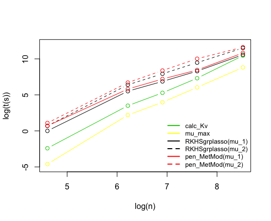
It appears that, the algorithms of these functions are of polynomial time with for the functions calcKv and mumax, and for the functions RKHSgrplasso and penMetMod.
Taking into account the results obtained for the prediction error and the values of in Example 2, in this example, only two values of the tuning parameter , and one value of the tuning parameter are considered.
The RKHS meta-models associated with the pair of values , are estimated using the RKHSMetMod function:
R> kernel <- "matern"; Dmax <- 3
R> gamma <- c(0.01); frc <- c(128,256)
R> res <- RKHSMetMod(Y, X, kernel, Dmax, gamma, frc, FALSE)
The prediction error and the empirical Sobol indices are then calculated for the obtained meta-models using the functions PredErr and SIemp:
R> mu <- vector(); mu[1] <- res[[1]]$mu; mu[2] <- res[[2]]$mu
R> Err <- PredErr(X, XT, YT, mu, gamma, res, kernel, Dmax)
R> SI <- SIemp(res, NULL)
The result of the prediction errors associated with the obtained estimators for two different values of are displayed in Table 9.
For equal to , we obtained smaller values of the prediction error, so as expected, the prediction quality improves by increasing the number of the observations . Table 10 gives the estimated empirical Sobol indices as well as their sum and the values of RE (see Equation (18)).
| sum | RE | |||||||||
|---|---|---|---|---|---|---|---|---|---|---|
Comparing the values of RE, we can see that the empirical Sobol indices are better estimated for n equal to , so as expected, the estimation of the Sobol indices is better for larger values of .
In Figure 2 the result of the estimation quality and the Sobol indices for the dataset with equal to , equal to , and are displayed.
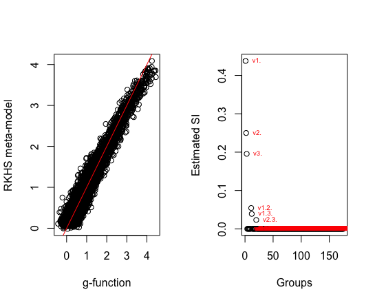
The line in red crosses the cloud of points as long as the values of the g-function are smaller than three. When the values of the g-function are greater than three, the estimator tends to underestimate the g-function.
4.2 Comparison examples
This section includes two examples. In the first example we reproduce an example from paper [\citeauthoryearGu, Palomo, and BergerGu et al.2019] and compare the prediction quality of the RKHS meta-model with the GP (Kriging) based meta-models from the RobusGaSP [\citeauthoryearGu, Palomo, and BergerGu et al.2019] and DiceKriging [\citeauthoryearRoustant, Ginsbourger, and DevilleRoustant et al.2012] packages.
The objective is to evaluate the quality of the RKHS estimated meta-model and to compare it with methods recently proposed for approximating complex models. In the first example we consider one-dimensional model and focuse on the comparison between the true model and the estimated meta-model. In the second example we reproduce an example from paper [\citeauthoryearRoustant, Ginsbourger, and DevilleRoustant et al.2012] which allows us to compare the prediction quality of the RKHS meta-model with the Kriging based meta-model from DiceKriging package, as well as the estimation quality of the Sobol indices in our package with the well-known package sensitivity.
For the sake of comparison between the three methods, the meta-models are calculated using the same experimental design and outputs and the same kernel function available in three packages is used. However, in packages RobustGaSP and DiceKriging the range parameter (see Table 1) in the kernel function is estimated by marginal posterior modes with the robust parameterization and by MLE with upper and lower bounds, respectively, while it is assumed to be fixed and set as in the RKHSMetaMod package.
Example 4.
"The modified sine wave function" [\citeauthoryearGu, Palomo, and BergerGu et al.2019].
We consider the -dimensional modified sine wave function defined over by:
The same experimental design as described in [\citeauthoryearGu, Palomo, and BergerGu
et al.2019] is considered: the design matrix is a sequence of equally spaced points on , and the response variable is calculated as :
R> X <- as.matrix(seq(0,1,1/11)); Y <- sinewave(X)
where sinewave function is defined in [\citeauthoryearGu, Palomo, and BergerGu
et al.2019].
We build the GP based meta-models by the RobustGaSP and the DiceKriging packages using the constant mean function and kernel Matérn :
R> library(RobustGaSP)
R> res.rgasp <- rgasp(design=X, response=Y, kerneltype="matern32")
R> library(DiceKriging)
R> res.km <- km(design=X, response=Y, covtype="matern32")
As , we have . We consider the grid of values of and .
The RKHS meta-models associated with the pair of values , , are estimated using the RKHSMetMod function:
R> kernel <- "matern"; Dmax <- 1
R> gamma <- c(0.2, 0.1, 0.01, 0.005,0)
R> frc <- c(4,8,16,32,64,128,256,512,1024)
R> res <- RKHSMetMod(Y, X, kernel, Dmax, gamma, frc, FALSE)
Given a testing dataset , the prediction errors associated with the obtained RKHS meta-models are calculated using the PredErr function, and the best RKHS meta-model is chosen to be the estimator of the model :
R> XT <- as.matrix(seq(0,1,1/11)); YT <- sinewave(XT)
R> Err <- PredErr(X, XT, YT, mu, gamma, res, kernel, Dmax)
To compare these three estimators in terms of the prediction quality, we perform prediction on test points, equally spaced in :
R> predictX <- as.matrix(seq(0,1,1/99))
R> #prediction with the GP based meta-models:
R> rgasp.predict <- predict(res.rgasp, predictX)
R> km.predict <- predict(res.km, predictX, type=’UK’)
R> #prediction with the best RKHS meta-model:
R> res.predict <- prediction(X, predictX, kernel, Dmax, res, Err)
The prediction results are plotted in Figure 3. The black circles that correspond to the prediction from the RKHSMetMod package are closer to the real output than the green and the blue circles corresponding to the predictive means from the RobustGaSP and DiceKriging packages.

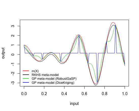
The meta-model results are plotted in Figure 4. The prediction from the RKHSMetaMod package plotted as the black curve is much more accurate as an estimate of the true function (plotted in red) than the predictive mean from the RobustGaSP and DiceKriging packages plotted as the blue and green curves, respectively. As already noted by [\citeauthoryearGu, Palomo, and BergerGu et al.2019], for that sine wave example, the meta-model from the DiceKriging package "degenerates to the fitted mean with spikes at the design points".
Example 5.
"A standard SA 8-dimensional example" [\citeauthoryearRoustant, Ginsbourger, and DevilleRoustant et al.2012].
We consider the -dimensional g-function of Sobol implemented in the package sensitivity: the function as defined in Equation (17) with coefficients . With these values of coefficients , the variables , , and explain of the variance of the function (see Table 11).
We consider the same experimental design as described in [\citeauthoryearRoustant, Ginsbourger, and DevilleRoustant
et al.2012]: the design matrices and are -point optimal Latin Hypercube Samples of the input variables generated by the optimumLHS function of package lhs, and the response variables and are calculated as , and using sobol.fun function of the package sensitivity:
R> n <- 80; d <- 8
R> library(lhs); X <- optimumLHS(n, d); XT <- optimumLHS(n, d)
R> library(sensitivity); Y <- sobol.fun(X); YT <- sobol.fun(XT)
Let us first consider the RKHS meta-model method. We set Dmax, and we consider the grid of values of , and .
The RKHS meta-models associated with the pair of values , , are estimated using the RKHSMetMod function:
R> kernel <- "matern"; Dmax <- 3
R> gamma <- c(0.2, 0.1, 0.01, 0.005,0)
R> frc <- c(4,8,16,32,64,128,256,512,1024)
R> res <- RKHSMetMod(Y, X, kernel, Dmax, gamma, frc, FALSE)
Given the testing dataset , the prediction errors associated with the obtained RKHS meta-models are calculated using PredErr function, and the best RKHS meta-model is chosen to be the estimator of the model . Finally, the Sobol indices are computed for the best RKHS meta-model using the function SIemp:
R> Err <- PredErr(X, XT, YT, mu, gamma, res, kernel, Dmax)
R> SI <- SIemp(res, Err)
Secondly, let us build the GP based meta-model. We use the km function of the package DiceKriging with the constant mean function and kernel Matérn :
R> library(DiceKriging)
R> res.km <- km(design = X, response = Y, covtype = "matern32")
The Sobol indices associated with the estimated GP based meta-model are calculated using fast99 function of the package sensitivity:
R> SI.km <- fast99(model = kriging.mean, factors = d, n = 1000,
+ q = "qunif", q.arg = list(min = 0, max = 1), m = res.km)
where kriging.mean function is defined in [\citeauthoryearRoustant, Ginsbourger, and DevilleRoustant
et al.2012].
The result of the estimation with the best RKHS meta-model and the Kriging based meta-model is drawn in Figure 5.

The black circles that correspond to the best RKHS meta-model are closer to the real output than the blue circles corresponding to the GP based meta-model from the DiceKriging package. Another way to evaluate the prediction quality of the estimated meta-models is to consider the mean square error of the fitted meta-model computed by . We obtained and for the Kriging based meta-model and the RKHS meta-model, respectively, which confirms the good behavior of the RKHS meta-model.
The estimated Sobol indices associated with the RKHS meta-model and the Kriging based meta-model are given in Table 11.
| sum | ||||||||||||
|---|---|---|---|---|---|---|---|---|---|---|---|---|
| 71.62 | 17.90 | 2.37 | 0.72 | 5.97 | 0.79 | 0.24 | 0.20 | 0.06 | 0.07 | 0.02 | 99.96 | |
| 75.78 | 17.42 | 1.71 | 0.47 | 4.00 | 0.05 | 0.07 | 0.28 | 0.09 | 0.00 | 0.00 | 99.87 | |
| 71.18 | 15.16 | 1.42 | 0.44 | 0.00 | 0.00 | 0.00 | 0.00 | 0.00 | 0.00 | 0.00 | 88.20 |
As shown, with RKHS meta-model, we obtained non-zero values for the interactions of order two. Concerning the main effects, excepting the first one, the estimated Sobol indices with the RKHS meta-model are closer to the true ones. However, the interactions of order three are ignored by both meta-models. For a general comparison of the estimation quality of the Sobol indices, one may consider the criterion RE defined in Equation (18), which is equal to for the Kriging based meta-model, and for the RKHS meta-model. Comparing the values of RE, we can point out that the Sobol indices are better estimated with the RKHS meta-model in that model.
5 Summary and discussion
In this paper, we proposed an R package, called RKHSMetaMod, that estimates a meta-model of a complex model . This meta-model belongs to a reproducing kernel Hilbert space constructed as a direct sum of Hilbert spaces [\citeauthoryearDurrande, Ginsbourger, Roustant, and CarraroDurrande et al.2013]. The estimation of the meta-model is carried out via a penalized least-squares minimization allowing both to select and estimate the terms in the Hoeffding decomposition, and therefore, to select the Sobol indices that are non-zero and estimate them [\citeauthoryearHuet and TaupinHuet and Taupin2017]. This procedure makes it possible to estimate the Sobol indices of high order, a point known to be difficult in practice. Using the convex optimization tools, RKHSMetaMod package implements two optimization algorithms: the minimization of the RKHS ridge group sparse criterion (13) and the RKHS group lasso criterion (14). Both of these algorithms rely on the Gram matrices , and their positive definiteness. Currently, the package considers only uniformly distributed input variables. If one is interested by another distribution of the input variables, it suffices to modify the calculation of the kernels , (see Equation (19)) in the function calcKv of this package (see Remark 3). The available kernels in the RKHSMetaMod package are: Gaussian kernel (with the fixed range parameter ), Matérn kernel (with the fixed range parameter ), Brownian kernel, quadratic kernel and linear kernel (see Table 1). With regard to the problem being under study, one may consider other kernels or kernels with different values of the range parameter and add them easily to the list of the kernels in the calcKv function. For the large values of and the calculation and storage of the eigenvalues and the eigenvectors of all the Gram matrices , require a lot of time and a very large amount of memory. In order to optimize the execution time and also the storage memory, except for a function that is written in R, all of the functions of RKHSMetaMod package are written using the efficient C++ libraries through RcppEigen and RcppGSL packages. These functions are then interfaced with the R environment in order to propose a user friendly package.
6 Supplementary materials
6.1 Appendix
Preliminary 1.
For , where is a symmetric matrix that does not depend on x, we have: if , and if .
Preliminary 2.
Let be a convex function. We have the following first order optimality condition:
This results from the fact that for all in both cases [\citeauthoryearGiraudGiraud2014].
6.1.1 RKHS construction
We begin this Section with a brief introduction to the RKHS. Let be a Hilbert space of real valued functions on a set . The space is a RKHS if for all the evaluation functionals are continuous. The Riesz representation Theorem ensures the existence of an unique element in verifying the property that where denotes the inner product in . It follows that for all , in , and , in , we have This allows to define the reproducing kernel of as The reproducing kernel is positive definite since it is symmetric, and for any , and , we have:
For more background on RKHS, we refer to various standard references such as [\citeauthoryearAronszajnAronszajn1950], [\citeauthoryearSaitohSaitoh1988], and [\citeauthoryearBerlinet and Thomas-AgnanBerlinet and
Thomas-Agnan2003].
In this work, the idea is to construct a RKHS such that any function in is decomposed as its Hoeffding decomposition, and therefore, any function in is a candidate to approximate the Hoeffding decomposition of .
To do so, the method of [\citeauthoryearDurrande, Ginsbourger, Roustant, and
CarraroDurrande et al.2013] as described below is used.
Let be a subset of . For each , we choose a RKHS and its associated kernel defined on the set such that the two following properties are satisfied:
- (i)
is measurable,
- (ii)
.
The property (ii) depends on the kernel , and the distribution of , . It is not very restrictive since it is satisfied, for example, for any bounded kernel.
The RKHS can be decomposed as a sum of two orthogonal sub-RKHS, where is the RKHS of zero mean functions, and is the RKHS of constant functions, The kernel associated with the RKHS is defined by:
| (19) |
Let then the ANOVA kernel is defined as follows:
For being the RKHS associated with the kernel , the RKHS associated with the ANOVA kernel is then defined by where denotes the inner product. According to this construction, any function satisfies decomposition (7), which is the Hoeffding decomposition of .
The regularity properties of the RKHS constructed as described above, depend on the set of the kernels (, ). This method allows us to choose different approximation spaces independently of the distribution of the input variables , by choosing different sets of kernels. While, as mentioned earlier, in the meta-modelling approach based on the polynomial Chaos expansion, according to the distribution of the input variables , a unique family of orthonormal polynomials is determined. Here, the distribution of the components of occurs only for the orthogonalization of the spaces , , and not in the choice of the RKHS, under the condition that properties (i) and (ii) are satisfied. This is one of the main advantages of this method compared to the method based on the truncated polynomial Chaos expansion where the smoothness of the approximation is handled only by the choice of the truncation [\citeauthoryearBlatman and SudretBlatman and Sudret2011].
6.1.2 RKHS group lasso algorithm
We consider the minimization of the RKHS group lasso criterion given by,
We begin with the constant term . The ordinary first derivative of the function at is equal to:
and therefore,
| (20) |
where denotes the i-th component of .
The next step is to calculate Since is convex and separable, we use a block coordinate descent algorithm, group by group . In the following, we fix a group , and we find the minimizer of with respect to for the given values of and , . Set
where
| (21) |
We aim to minimize with respect to . Let be the sub-differential of with respect to :
The first order optimality condition (see Preliminary (2)) ensures the existence of fulfilling,
| (22) |
Using the sub-differential definition (see Preliminary 1), we obtain:
and,
Let be the minimizer of . The sub-differential equations above give the two following cases:
Case 1. If , then there exists such that and it fulfils Equation (22), .
Therefore, the necessary and sufficient condition for which the solution is the optimal one is
Case 2. If , then and it fulfils Equation (22),
We obtain then,
| (23) |
Since appears in both sides of the Equation (23), a numerical procedure is needed:
Proposition 1.
For let . There exists a non-zero solution to Equation (23) if and only if there exists such that
| (24) |
Then .
Proof
If there exists a non-zero solution to Equation (23), then since is positive definite. Take then and, for such Equation (24) is satisfied. Conversely, if there exists such that Equation (24) is satisfied, then and Therefore, which is Equation (23) calculated in .
Remark 5.
Define with , then has a unique solution, denoted , which leads to calculate .
Proof
For we have , since ; and for we have , since and .
Moreover, we have , which is equal to with and . The first derivative of in is obtained by . Finally, by simple calculations we get,
Therefore is an increasing function of , and the proof is complete.
In order to calculate and so , we use Algorithm 4 which is a part of the RKHS group lasso Algorithm 1 when .
6.1.3 Computational cost
The complexity for the matrices , is equal to , which is given by the singular value decomposition to get eigenvalues and eigenvectors of each . Supposing that the matrices , was first created and are already stored, the complexity for the constant term is given by the second term in equation (20), which is equal to . Given , the complexity for , , is given by the backsolving of to get , which is equal to . The computation of is done using Brent-Dekker method implemented as function gsl_root_fsolver_brent from [\citeauthoryearGalassi, Davies, Theiler, Gough, Jungman, Alken, Booth, Rossi, and UlerichGalassi et al.2018]. This method combines an interpolation strategy with the bisection algorithm and takes iterations to converge, where is the number of steps that the bisection algorithm would take.
6.1.4 RKHS ridge group sparse algorithm
We consider the minimization of the RKHS ridge group sparse criterion:
The constant term is estimated as in the RKHS group lasso algorithm. In order to calculate , we use once again the block coordinate descent algorithm group by group . In the following, we fix a group , and we find the minimizer of with respect to for given values of and , . We aim at minimizing with respect to ,
where is defined by (21).
Let be the sub-differential of with respect to ,
According to the first order optimality condition (see Preliminary 2), we know that there exists and such that,
| (25) |
The sub-differential definition (see Preliminary 1) gives:
and,
Let be the minimizer of the .
Using the sub-differential equations above, the estimator , is obtained following the two cases below:
Case 1. If , then there exists such that and it fulfils Equation (25),
with , . Set and,
Then the solution to Equation (25) is zero if and only if .
Case 2. If , then we have , and fulfilling Equation (25),
that is,
| (26) |
In this case the calculation of needs a numerical algorithm.
Proposition 2.
(Proposition 8.4 in [\citeauthoryearHuet and TaupinHuet and Taupin2017]) For , let . If , there exists a non zero solution to Equation (26) if and only if there exists such that Then .
Proof
The proof is given in [\citeauthoryearHuet and TaupinHuet and Taupin2017].
6.1.5 Computational cost
The complexity for the matrices , and the constant term is the same as for RKHS group lasso algorithm. Given , the complexity for , , is given by the backsolving of to get , which is equal to . The computation of , is insured using a combination of three methods: first we implement a modified version of Newton’s method, if it does not achieve the convergence second we implement a version of the Hybrid algorithm and if it does not achieve the convergence, third we implement a version of the discrete Newton algorithm called Broyden algorithm. These methods are implemented as functions gsl_multiroot_fdfsolver_gnewton, gsl_multiroot_fsolver_hybrids, and gsl_multiroot_fsolver_broyden from [\citeauthoryearGalassi, Davies, Theiler, Gough, Jungman, Alken, Booth, Rossi, and UlerichGalassi et al.2018], respectively. These methods converge fast in general, and for big enough their complexity is dominated by .
6.2 Overview of the RKHSMetaMod functions
In the R environment, one can install and load the RKHSMetaMod package by using the following commands:
Example 6.
install.packages("RKHSMetaMod") library("RKHSMetaMod")
The optimization problems in this package are solved using block coordinate descent algorithm which requires various computational algorithms including generalized Newton, Broyden and Hybrid methods. In order to gain the efficiency in terms of the calculation time and be able to deal with high dimensional problems, the computationally efficient tools of C++ packages Eigen [\citeauthoryearGuennebaud, Jacob, et al.Guennebaud et al.2010] and GSL [\citeauthoryearGalassi, Davies, Theiler, Gough, Jungman, Alken, Booth, Rossi, and UlerichGalassi et al.2018] via RcppEigen [\citeauthoryearBates and EddelbuettelBates and Eddelbuettel2013] and RcppGSL [\citeauthoryearEddelbuettel and FrancoisEddelbuettel and Francois2019] packages are used in the RKHSMetaMod package. For different examples of usage of RcppEigen and RcppGSl functions see the work by [\citeauthoryearEddelbuettelEddelbuettel2013].
The complete documentation of RKHSMetaMod package is available from CRAN [\citeauthoryearKamariKamari2019]. Here, a brief documentation of some of its main and companion functions is presented in the next two Sections.
6.2.1 Main RKHSMetaMod functions
Let us begin by introducing some notations. For a given Dmax, let be the set of parts of with dimension to Dmax. The cardinal of is denoted by
RKHSMetMod function:
For a given value of Dmax and a chosen kernel (see Table 1), this function calculates the Gram matrices , , and produces a sequence of estimators associated with a given grid of values of tuning parameters , i.e. the solutions to the RKHS ridge group sparse (if ) or the RKHS group lasso problem (if ). Table 12 gives a summary of all the input arguments of the RKHSMetMod function as well as the default values for non-mandatory arguments.
| Input parameter | Description |
|---|---|
| Y | Vector of the response observations of size . |
| X | Matrix of the input observations with rows and columns. Rows correspond to the observations and columns correspond to the variables. |
| kernel | Character, indicates the type of the kernel (see Table 1) chosen to construct the RKHS . |
| Dmax | Integer, between and , indicates the maximum order of interactions considered in the RKHS meta-model: Dmax is used to consider only the main effects, Dmax to include the main effects and the second-order interactions, and so on. |
| gamma | Vector of non-negative scalars, values of the tuning parameter in decreasing order. If the function solves the RKHS group lasso optimization problem and for it solves the RKHS ridge group sparse optimization problem. |
| frc | Vector of positive scalars. Each element of the vector sets a value to the tuning parameter : . The value (see Equation (16)) is calculated inside the program. |
| verbose | Logical. Set as TRUE to print: the group for which the correction of the Gram matrix is done (see Section 3.1), and for each pair of the tuning parameters : the number of current iteration, active groups and convergence criteria. It is set as FALSE by default. |
The RKHSMetMod function returns a list of components, with being equal to the number of pairs of the tuning parameters , i.e. . Each component of the list is a list of three components "mu", "gamma" and "Meta-Model":
- •
mu: value of the tuning parameter if , or if .
- •
gamma: value of the tuning parameter .
- •
Meta-Model: a RKHS ridge group sparse or RKHS group lasso object associated with the tuning parameters mu and gamma. Table 13 gives a summary of all arguments of the output "Meta-Model" of RKHSMetMod function.
| Output parameter | Description |
|---|---|
| intercept | Scalar, estimated value of intercept. |
| teta | Matrix with vMax rows and columns. Each row of the matrix is the estimated vector for vMax. |
| fit.v | Matrix with rows and vMax columns. Each row of the matrix is the estimated value of . |
| fitted | Vector of size , indicates the estimator of . |
| Norm.n | Vector of size vMax, estimated values for the empirical -norm. |
| Norm.H | Vector of size vMax, estimated values for the Hilbert norm. |
| supp | Vector of active groups. |
| Nsupp | Vector of the names of the active groups. |
| SCR | Scalar equals to . |
| crit | Scalar indicates the value of the penalized criterion. |
| gamma.v | Vector of size vMax, coefficients of the empirical -norm. |
| mu.v | Vector of size vMax, coefficients of the Hilbert norm. |
| iter | List of two components: maxIter, and the number of iterations until the convergence is achieved. |
| convergence | TRUE or FALSE. Indicates whether the algorithm has converged or not. |
| RelDiffCrit | Scalar, value of the first convergence criterion at the last iteration, i.e. . |
| RelDiffPar | Scalar, value of the second convergence criterion at the last iteration, i.e. . |
RKHSMetModqmax function:
For a given value of Dmax and a chosen kernel (see Table 1), this function calculates the Gram matrices , ; determines , reffered to as , for which the number of groups in the support of the RKHS group lasso solution is equal to ; and produces a sequence of estimators associated with the tuning parameter and a grid of values of the tuning parameter . All the estimators produced by this function have at most groups in their support. This function has the following input arguments:
-
, , kernel, Dmax, gamma, verbose (see Table 12).
-
qmax: integer, the maximum number of groups in the support of the obtained solution.
-
Num: integer, to restrict the number of different values of the tuning parameter to be evaluated in the RKHS group lasso algorithm until it achieves . For example, if Num equals , the program is implemented for three different values of :
where is the number of groups in the support of the solution of the RKHS group lasso problem, Algorithm 1, associated with .
If Num, the path to cover the interval is detailed in Algorithm 3.
The RKHSMetModqmax function returns a list of three components "mus", "qs", and "MetaModel":
- •
mus: vector of all values of in Algorithm 3.
- •
qs: vector with the same length as mus. Each element of the vector shows the number of groups in the support of the RKHS meta-model obtained by solving RKHS group lasso problem for an element in mus.
- •
MetaModel: list with the same length as the vector gamma. Each component of the list is a list of three components "mu", "gamma" and "Meta-Model":
- –
mu: value of .
- –
gamma: element of the input vector gamma associated with the estimated "Meta-Model".
- –
Meta-Model: a RKHS ridge group sparse or RKHS group lasso object associated with the tuning parameters mu and gamma (see Table 13).
- –
6.2.2 Companion functions
calcKv function:
For a given value of Dmax and a chosen kernel (see Table 1), this function calculates the Gram matrices , , and returns their associated eigenvalues and eigenvectors. This function has,
- •
four mandatory input arguments:
- –
, , kernel, Dmax (see Table 12).
- –
- •
three facultative input arguments:
- –
correction: logical, set as TRUE to make correction to the matrices (see Section 3.1). It is set as TRUE by default.
- –
verbose: logical, set as TRUE to print the group for which the correction is done. It is set as TRUE by default.
- –
tol: scalar to be chosen small, set as by default.
- –
The calcKv function returns a list of two components "kv" and "names.Grp":
- •
kv: list of vMax components, each component is a list of,
- –
Evalues: vector of eigenvalues.
- –
Q: matrix of eigenvectors.
- –
- •
names.Grp: vector of group names of size vMax.
RKHSgrplasso function:
For a given value of the tuning parameter , this function fits the solution to the RKHS group lasso optimization problem by implementing Algorithm 1. This function has,
- •
three mandatory input arguments:
- •
two facultative input arguments:
- –
maxIter: integer, to set the maximum number of loops through all groups. It is set as by default.
- –
verbose: logical, set as TRUE to print the number of current iteration, active groups and convergence criterion. It is set as FALSE by default.
- –
This function returns a RKHS group lasso object associated with the tuning parameter . Its output is a list of components:
- •
intercept, teta, fit.v, fitted, Norm.H, supp, Nsupp, SCR, crit, MaxIter, convergence, RelDiffCrit, and RelDiffPar (see Table 13).
mumax function:
This function calculates the value defined in Equation (16). It has two mandatory input arguments: the response vector , and the list matZ of the eigenvalues and eigenvectors of the positive definite Gram matrices for vMax. This function returns the value.
penMetMod function:
This function produces a sequence of the RKHS meta-models associated with a given grid of values of the tuning parameters . Each RKHS meta-model in the sequence is the solution to the RKHS ridge group sparse optimization problem (obtained by implementing Algorithm 2) associated with a pair of values of in the grid of values of . This function has,
- •
seven mandatory input arguments:
- –
(see Table 12).
- –
gamma: vector of positive scalars. Values of the penalty parameter in decreasing order.
- –
Kv: list of the eigenvalues and the eigenvectors of the positive definite Gram matrices for vMax and their associated group names (output of the function calcKv).
- –
mu: vector of positive scalars. Values of the tuning parameter in decreasing order.
- –
resg: list of the RKHS group lasso objects associated with the components of "mu", used as initial parameters at Step .
- –
gama_v and mu_v: vector of vMax positive scalars. These two inputs are optional. They are provided to associate the weights to the two penalty terms in the RKHS ridge group sparse criterion (13). In order to consider no weights, i.e. all the weights are equal to one, we set these two inputs to scalar zero.
- –
- •
three facultative input arguments:
- –
- –
verbose: logical, set as TRUE to print for each pair of the tuning parameters , the number of current iteration, active groups and convergence criterion. It is set as FALSE by default.
- –
calcStwo: logical, set as TRUE to execute Step . It is set as FALSE by default.
The function penMetMod returns a list of components, with being equal to the number of pairs of the tuning parameters . Each component of the list is a list of three components "mu", "gamma" and "Meta-Model":
- •
mu: positive scalar, an element of the input vector "mu" associated with the estimated "Meta-Model".
- •
gamma: positive scalar, an element of the input vector "gamma" associated with the estimated "Meta-Model".
- •
Meta-Model: a RKHS ridge group sparse object associated with the tuning parameters mu and gamma (see Table 13).
PredErr function:
By considering a testing dataset, this function calculates the prediction errors for the obtained RKHS meta-models. This function has eight mandatory input arguments:
-
, gamma, kernel, Dmax (see Table 12).
-
: matrix of observations of the testing dataset with rows and columns.
-
: vector of response observations of the testing dataset of size .
-
mu: vector of positive scalars. Values of the tuning parameter in decreasing order.
-
res: list of the estimated RKHS meta-models for the learning dataset associated with the tuning parameters (it could be the output of one of the functions RKHSMetMod or penMetMod).
Note that, the same kernel and Dmax have to be chosen as the ones used for the learning dataset.
The function PredErr returns a matrix of the prediction errors. Each element of the matrix corresponds to the prediction error of one RKHS meta-model in "res".
prediction function:
This function calculates the predicted values for a new dataset based on the best RKHS meta-model estimator. It has six input arguments:
-
X, kernel, Dmax (see Table 12).
-
Xnew: matrix of new observations with rows and columns.
-
res: list of the estimated RKHS meta-models for a learning dataset associated with the tuning parameters (it could be the output of one of the functions RKHSMetMod, RKHSMetModqmax or penMetMod).
-
Err: matrix of the prediction errors associated with the RKHS meta-models in "res" (output of the function PredErr).
The function prediction returns a vector of the predicted values based on the best RKHS meta-model estimator in "res". This function is available at GitHub.
SIemp function:
For each RKHS meta-model , this function calculates the empirical Sobol indices for all the groups that are active in the support of . This function has two input arguments:
-
res: list of the estimated meta-models using RKHS ridge group sparse or RKHS group lasso algorithms (it could be the output of one of the functions RKHSMetMod, RKHSMetModqmax or penMetMod).
-
ErrPred: matrix or NULL. If matrix, each element of the matrix corresponds to the prediction error of a RKHS meta-model in "res" (output of the function PredErr). Set as NULL by default.
The empirical Sobol indices are then calculated for each RKHS meta-model in "res", and a list of vectors of the Sobol indices is returned. If the argument "ErrPred" is the matrix of the prediction errors, the vector of empirical Sobol indices is returned for the best RKHS meta-model in the "res".
References
- \citeauthoryearAronszajnAronszajn1950 Aronszajn, N. (1950). Theory of Reproducing Kernels. Transactions of the American Mathematical Society 68(3), 337–404.
- \citeauthoryearBates and EddelbuettelBates and Eddelbuettel2013 Bates, D. and D. Eddelbuettel (2013). Fast and Elegant Numerical Linear Algebra Using the RcppEigen Package. Journal of Statistical Software 52(5), 1–24.
- \citeauthoryearBerlinet and Thomas-AgnanBerlinet and Thomas-Agnan2003 Berlinet, A. and C. Thomas-Agnan (2003). Reproducing Kernel Hilbert Spaces in Probability and Statistics. Springer US.
- \citeauthoryearBlatman and SudretBlatman and Sudret2011 Blatman, G. and B. Sudret (2011). Adaptive sparse polynomial chaos expansion based on least angle regression. Journal of computational Physics 230, 2345–2367.
- \citeauthoryearBoyd, Parikh, Chu, Peleato, and EcksteinBoyd et al.2011 Boyd, S., N. Parikh, E. Chu, B. Peleato, and J. Eckstein (2011, January). Distributed Optimization and Statistical Learning via the Alternating Direction Method of Multipliers. Found. Trends Mach. Learn. 3(1), 1–122.
- \citeauthoryearBubeckBubeck2015 Bubeck, S. (2015, November). Convex Optimization: Algorithms and Complexity. Found. Trends Mach. Learn. 8(3-4), 231–357.
- \citeauthoryearCarnellCarnell2021 Carnell, R. (2021). lhs: Latin Hypercube Samples. R package version 1.1.3.
- \citeauthoryearDancik and DormanDancik and Dorman2008 Dancik, G. M. and K. S. Dorman (2008). mlegp: statistical analysis for computer models of biological systems using R. Bioinformatics 24(17), 1966.
- \citeauthoryearDurrande, Ginsbourger, and RoustantDurrande et al.2012 Durrande, N., D. Ginsbourger, and O. Roustant (2012, 4). Additive Covariance kernels for high-dimensional Gaussian Process modeling. Annales de la faculté des sciences de Toulouse Mathématiques 21(3), 481–499.
- \citeauthoryearDurrande, Ginsbourger, Roustant, and CarraroDurrande et al.2013 Durrande, N., D. Ginsbourger, O. Roustant, and L. Carraro (2013). ANOVA kernels and RKHS of zero mean functions for model-based sensitivity analysis. Journal of Multivariate Analysis 115, 57 – 67.
- \citeauthoryearEddelbuettelEddelbuettel2013 Eddelbuettel, D. (2013). Seamless R and C++ Integration with Rcpp. Springer Publishing Company, Incorporated.
- \citeauthoryearEddelbuettel and FrancoisEddelbuettel and Francois2019 Eddelbuettel, D. and R. Francois (2019). RcppGSL: ’Rcpp’ Integration for ’GNU GSL’ Vectors and Matrices. R package version 0.3.7.
- \citeauthoryearFuFu1998 Fu, W. J. (1998). Penalized Regressions: The Bridge versus the Lasso. Journal of Computational and Graphical Statistics 7(3), 397–416.
- \citeauthoryearGalassi, Davies, Theiler, Gough, Jungman, Alken, Booth, Rossi, and UlerichGalassi et al.2018 Galassi, M., J. Davies, J. Theiler, B. Gough, G. Jungman, P. Alken, M. Booth, F. Rossi, and R. Ulerich (2018). GNU Scientific Library Reference Manual.
- \citeauthoryearGiraudGiraud2014 Giraud, C. (2014). Introduction to High-Dimensional Statistics. Chapman & Hall/CRC Monographs on Statistics & Applied Probability. Taylor & Francis.
- \citeauthoryearGuGu2019 Gu, M. (2019). Jointly Robust Prior for Gaussian Stochastic Process in Emulation, Calibration and Variable Selection. Bayesian Analysis 14(3), 857 – 885.
- \citeauthoryearGu, Palomo, and BergerGu et al.2019 Gu, M., J. Palomo, and O. Berger, James (2019). RobustGaSP: Robust Gaussian Stochastic Process Emulation in R. The R Journal 11(1), 112.
- \citeauthoryearGu, Wang, and BergerGu et al.2018 Gu, M., X. Wang, and J. O. Berger (2018). Robust Gaussian stochastic process emulation. The Annals of Statistics 46(6A), 3038 – 3066.
- \citeauthoryearGuennebaud, Jacob, et al.Guennebaud et al.2010 Guennebaud, G., B. Jacob, et al. (2010). Eigen v3. http://eigen.tuxfamily.org.
- \citeauthoryearHastie, Tibshirani, and WainwrightHastie et al.2015 Hastie, T., R. Tibshirani, and M. Wainwright (2015). Statistical Learning with Sparsity: The Lasso and Generalizations. Chapman & Hall/CRC.
- \citeauthoryearHomma and SaltelliHomma and Saltelli1996 Homma, T. and A. Saltelli (1996). Importance measures in global sensitivity analysis of nonlinear models. Reliability Engineering & System Safety 52(1), 1 – 17.
- \citeauthoryearHuet and TaupinHuet and Taupin2017 Huet, S. and M.-L. Taupin (2017). Metamodel construction for sensitivity analysis. ESAIM: Procs 60, 27–69.
- \citeauthoryearKamariKamari2019 Kamari, H. (2019). RKHSMetaMod: Ridge Group Sparse Optimization Problem for Estimation of a Meta Model Based on Reproducing Kernel Hilbert Spaces. R package version 1.1.
- \citeauthoryearKennedy and O’HaganKennedy and O’Hagan2000 Kennedy, M. C. and A. O’Hagan (2000). Bayesian Calibration of Computer Models. Journal of the Royal Statistical Society, Series B, Methodological 63, 425–464.
- \citeauthoryearKimeldorf and WahbaKimeldorf and Wahba1970 Kimeldorf, G. S. and G. Wahba (1970, 04). A Correspondence Between Bayesian Estimation on Stochastic Processes and Smoothing by Splines. Ann. Math. Statist. 41(2), 495–502.
- \citeauthoryearKleijnenKleijnen2007 Kleijnen, J. P. C. (2007). Design and Analysis of Simulation Experiments (1st ed.). Springer Publishing Company, Incorporated.
- \citeauthoryearKleijnenKleijnen2009 Kleijnen, J. P. C. (2009). Kriging metamodeling in simulation: A review. European Journal of Operational Research 192(3), 707 – 716.
- \citeauthoryearLe Gratiet, Cannamela, and IoossLe Gratiet et al.2014 Le Gratiet, L., C. Cannamela, and B. Iooss (2014). A Bayesian Approach for Global Sensitivity Analysis of (Multifidelity) Computer Codes. SIAM/ASA Journal on Uncertainty Quantification 2(1), 336–363.
- \citeauthoryearLe Gratiet, Marelli, and SudretLe Gratiet et al.2017 Le Gratiet, L., S. Marelli, and B. Sudret (2017). Metamodel-Based Sensitivity Analysis: Polynomial Chaos Expansions and Gaussian Processes, pp. 1289–1325. Cham: Springer International Publishing.
- \citeauthoryearLin and ZhangLin and Zhang2006 Lin, Y. and H. H. Zhang (2006, 10). Component selection and smoothing in multivariate nonparametric regression. Ann. Statist. 34(5), 2272–2297.
- \citeauthoryearLiu, Wasserman, and LaffertyLiu et al.2009 Liu, H., L. Wasserman, and J. D. Lafferty (2009). Nonparametric regression and classification with joint sparsity constraints. In D. Koller, D. Schuurmans, Y. Bengio, and L. Bottou (Eds.), Advances in Neural Information Processing Systems 21, pp. 969–976. Curran Associates, Inc.
- \citeauthoryearMarrel, Iooss, Laurent, and RoustantMarrel et al.2009 Marrel, A., B. Iooss, B. Laurent, and O. Roustant (2009). Calculations of Sobol indices for the Gaussian process metamodel. Reliability Engineering & System Safety 94(3), 742 – 751.
- \citeauthoryearMebane and SekhonMebane and Sekhon2011 Mebane, W. and J. Sekhon (2011). Genetic Optimization Using Derivatives: The rgenoud Package for R. Journal of Statistical Software, Articles 42(11), 1–26.
- \citeauthoryearMeierMeier2020 Meier, L. (2020). grplasso: Fitting User-Specified Models with Group Lasso Penalty. R package version 0.4-7.
- \citeauthoryearMeier, van de Geer, and BühlmannMeier et al.2008 Meier, L., S. van de Geer, and P. Bühlmann (2008). The group lasso for logistic regression. Journal of the Royal Statistical Society. Series B 70(1), 53–71.
- \citeauthoryearMeier, van de Geer, and BühlmannMeier et al.2009 Meier, L., S. van de Geer, and P. Bühlmann (2009, 12). High-dimensional additive modeling. Ann. Statist. 37(6B), 3779–3821.
- \citeauthoryearOakley and O’HaganOakley and O’Hagan2004 Oakley, J. E. and A. O’Hagan (2004). Probabilistic sensitivity analysis of complex models: a Bayesian approach. Journal of the Royal Statistical Society: Series B (Statistical Methodology) 66(3), 751–769.
- \citeauthoryearRaskutti, Wainwright, and YuRaskutti et al.2009 Raskutti, G., M. J. Wainwright, and B. Yu (2009). Lower bounds on minimax rates for nonparametric regression with additive sparsity and smoothness. In Advances in Neural Information Processing Systems.
- \citeauthoryearRaskutti, Wainwright, and YuRaskutti et al.2012 Raskutti, G., M. J. Wainwright, and B. Yu (2012, February). Minimax-optimal Rates for Sparse Additive Models over Kernel Classes via Convex Programming. J. Mach. Learn. Res. 13(1), 389–427.
- \citeauthoryearRavikumar, Lafferty, Liu, and WassermanRavikumar et al.2009 Ravikumar, P., J. Lafferty, H. Liu, and L. Wasserman (2009). Sparse additive models. Journal of the Royal Statistical Society: Series B (Statistical Methodology) 71(5), 1009–1030.
- \citeauthoryearRoustant, Ginsbourger, and DevilleRoustant et al.2012 Roustant, O., D. Ginsbourger, and Y. Deville (2012). DiceKriging, DiceOptim: Two R Packages for the Analysis of Computer Experiments by Kriging-Based Metamodeling and Optimization. Journal of Statistical Software, Articles 51(1), 1–55.
- \citeauthoryearSaitohSaitoh1988 Saitoh, S. (1988). Theory of reproducing kernels and its applications. Pitman research notes in mathematics series. Longman Scientific & Technical.
- \citeauthoryearSaltelliSaltelli2002 Saltelli, A. (2002). Making best use of model evaluations to compute sensitivity indices. Computer Physics Communications 145(2), 280 – 297.
- \citeauthoryearSaltelli, Chan, and ScottSaltelli et al.2009 Saltelli, A., K. Chan, and E. Scott (2009). Sensitivity Analysis. Wiley.
- \citeauthoryearSaltelli, Tarantola, and ChanSaltelli et al.1999 Saltelli, A., S. Tarantola, and K. P.-S. Chan (1999). A Quantitative Model-Independent Method for Global Sensitivity Analysis of Model Output. Technometrics 41(1), 39–56.
- \citeauthoryearSchoutensSchoutens2000 Schoutens, W. (2000). Stochastic Processes and Orthogonal Polynomials. Lecture Notes in Statistics. Springer New York.
- \citeauthoryearSobolSobol1993 Sobol, I. M. (1993). Sensitivity Estimates for Nonlinear Mathematical Models. In Sensitivity Estimates for Nonlinear Mathematical Models.
- \citeauthoryearSoize and GhanemSoize and Ghanem2004 Soize, C. and R. Ghanem (2004). Physical Systems with Random Uncertainties: Chaos Representations with Arbitrary Probability Measure. SIAM Journal on Scientific Computing 26(2), 395–410.
- \citeauthoryearSudretSudret2008 Sudret, B. (2008). Global sensitivity analysis using polynomial chaos expansions. Reliability Engineering & System Safety 93(7), 964 – 979. Bayesian Networks in Dependability.
- \citeauthoryearVan der VaartVan der Vaart1998 Van der Vaart, A. W. (1998). Asymptotic Statistics. Cambridge Series in Statistical and Probabilistic Mathematics. Cambridge University Press.
- \citeauthoryearWelch, Buck, Sacks, Wynn, Mitchell, and MorrisWelch et al.1992 Welch, W. J., R. J. Buck, J. Sacks, H. P. Wynn, T. J. Mitchell, and M. D. Morris (1992). Screening, Predicting, and Computer Experiments. Technometrics 34(1), 15–25.
- \citeauthoryearWienerWiener1938 Wiener, N. (1938). The Homogeneous Chaos. American Journal of Mathematics 60(4), 897–936.
- \citeauthoryearYang and ZouYang and Zou2015 Yang, Y. and H. Zou (2015, November). A Fast Unified Algorithm for Solving Group-lasso Penalize Learning Problems. Statistics and Computing 25(6), 1129–1141.
- \citeauthoryearYang, Zou, and BhatnagarYang et al.2020 Yang, Y., H. Zou, and S. Bhatnagar (2020). gglasso: Group Lasso Penalized Learning Using a Unified BMD Algorithm. R package version 1.5.
- \citeauthoryearYuan and LinYuan and Lin2006 Yuan, M. and Y. Lin (2006). Model selection and estimation in regression with grouped variables. Journal of the Royal Statistical Society: Series B (Statistical Methodology) 68(1), 49–67.