跳到论文正文
W Papers独立论文阅读器 arXiv:1905.13547 论文正文 计算阅读时间 · 0%
引用这篇论文根据当前论文元数据生成,正式投稿前建议核对。


License: arXiv.org perpetual non-exclusive license
arXiv:1905.13547v4 [cs.LG] 01 May 2020

Learning Robust Controllers for Linear Quadratic Systems
with Multiplicative Noise via Policy GradientThanks: The authors are with the Control, Optimization, and Networks lab, UT Dallas, The United States ({benjamin.gravell, tyler.summers}@utdallas.edu), and the Delft Center for Systems and Control, TU Delft, The Netherlands (P.MohajerinEsfahani@tudelft.nl). This material is based on work supported by the Army Research Office under grant W911NF-17-1-0058.

Benjamin Gravell , Peyman Mohajerin Esfahani and Tyler Summers
Date: August 11, 2026
Abstract.

The linear quadratic regulator (LQR) problem has reemerged as an important theoretical benchmark for reinforcement learning-based control of complex dynamical systems with continuous state and action spaces. In contrast with nearly all recent work in this area, we consider multiplicative noise models, which are increasingly relevant because they explicitly incorporate inherent uncertainty and variation in the system dynamics and thereby improve robustness properties of the controller. Robustness is a critical and poorly understood issue in reinforcement learning; existing methods which do not account for uncertainty can converge to fragile policies or fail to converge at all. Additionally, intentional injection of multiplicative noise into learning algorithms can enhance robustness of policies, as observed in ad hoc work on domain randomization. Although policy gradient algorithms require optimization of a non-convex cost function, we show that the multiplicative noise LQR cost has a special property called gradient domination, which is exploited to prove global convergence of policy gradient algorithms to the globally optimum control policy with polynomial dependence on problem parameters. Results are provided both in the model-known and model-unknown settings where samples of system trajectories are used to estimate policy gradients.

1. Introduction

Reinforcement learning-based control has recently achieved impressive successes in games [47, 48] and simulators [41]. But these successes are significantly more challenging to translate to complex physical systems with continuous state and action spaces, safety constraints, and non-negligible operation and failure costs that demand data efficiency. An intense and growing research effort is creating a large array of models, algorithms, and heuristics for approaching the myriad of challenges arising from these systems. To complement a dominant trend of more computationally focused work, the canonical linear quadratic regulator (LQR) problem in control theory has reemerged as an important theoretical benchmark for learning-based control [45, 17]. Despite its long history, there remain fundamental open questions for LQR with unknown models, and a foundational understanding of learning in LQR problems can give insight into more challenging problems.

Almost all recent work on learning in LQR problems has utilized either deterministic or additive noise models [45, 17, 19, 12, 20, 1, 35, 51, 2, 53, 38, 54], but here we consider multiplicative noise models. In control theory, multiplicative noise models have been studied almost as long as their deterministic and additive noise counterparts [56, 16], although this area is somewhat less developed and far less widely known. We believe the study of learning in LQR problems with multiplicative noise is important for three reasons. First, this class of models is much richer than deterministic or additive noise while still allowing exact solutions when models are known, which makes it a compelling additional benchmark [55, 4, 8]. Second, they explicitly incorporate model uncertainty and inherent stochasticity, thereby improving robustness properties of the controller. Robustness is a critical and poorly understood issue in reinforcement learning; existing methods which do not account for uncertainty can converge to fragile policies or fail to converge at all [4, 34, 9]. Additionally, intentional injection of multiplicative noise into learning algorithms is known to enhance robustness of policies from ad hoc work on domain randomization [49]. Third, in emerging difficult-to-model complex systems where learning-based control approaches are perhaps most promising, multiplicative noise models are increasingly relevant; examples include networked systems with noisy communication channels [3, 25], modern power networks with large penetration of intermittent renewables [15, 40], turbulent fluid flow [37], and neuronal brain networks [13].

1.1. Related literature

Multiplicative noise LQR problems have been studied in control theory since the 1960s [56]. Since then a line of research parallel to deterministic and additive noise has developed, including basic stability and stabilizability results [55], semidefinite programming formulations [18, 10, 36], robustness properties [16, 8, 27, 6, 24], and numerical algorithms [7]. This line of research is less widely known perhaps because much of it studies continuous time systems, where the heavy machinery required to formalize stochastic differential equations is a barrier to entry for a broad audience. Multiplicative noise models are well-poised to offer data-driven model uncertainty representations and enhanced robustness in learning-based control algorithms and complex dynamical systems and processes. A related line of research which has seen recent activity is on learning optimal control of Markovian jump linear systems with unknown dynamics and noise distributions [46, 29], which under certain assumptions form a special case of the multiplicative noise system we analyze in this work.

In contrast to classical work on system identification and adaptive control, which has a strong focus on asymptotic results, more recent work has focused on non-asymptotic analysis using newly developed mathematical tools from statistics and machine learning. There remain fundamental open problems for learning in LQR problems, with several addressed only recently, including non-asymptotic sample complexity [17, 51], regret bounds [1, 2, 38], and algorithmic convergence [19]. Alternatives to reinforcement learning include other data-driven model-free optimal control schemes [23, 5] and those leveraging the behavioral framework [39, 42]. Subspace identification methods offer a model-based generalization to the output feedback setting [30].

1.2. Our contributions

In §2 we establish the multiplicative noise LQR problem and motivate its study via a connection to robust stability. We then give several fundamental results for policy gradient algorithms on linear quadratic problems with multiplicative noise. Our main contributions are as follows, which can be viewed as a generalization of the recent results of Fazel et al. [19] for deterministic LQR to multiplicative noise LQR:

  • •

    In §3 we show that although the multiplicative noise LQR cost is generally non-convex, it has a special property called gradient domination, which facilitates its optimization (Lemmas 3.1 and 3.3).

  • •

    In particular, in §4 the gradient domination property is exploited to prove global convergence of three policy gradient algorithm variants (namely, exact gradient descent, “natural” gradient descent, and Gauss-Newton/policy iteration) to the globally optimum control policy with a rate that depends polynomially on problem parameters (Theorems 4.1, 4.2, and 4.3).

  • •

    Furthermore, in §5 we show that a model-free policy gradient algorithm, where the gradient is estimated from trajectory data (“rollouts”) rather than computed from model parameters, also converges globally (with high probability) with an appropriate exploration scheme and sufficiently many samples (polynomial in problem data) (Theorem 5.1).

In comparison with the deterministic dynamics studied by [19], we make the following novel technical contributions:

  • •

    We quantify the increase in computational burden of policy gradient methods due to the presence of multiplicative noise, which is evident from the bounds developed in Appendices B and C. The noise acts to reduce the step size and thus convergence rate, and increases the required number of samples and rollout length in the model-free setting.

  • •

    A covariance dynamics operator ℱK\mathcal{F}_{K} is established for multiplicative noise systems with a more complicated form than the deterministic case. This necessitated a more careful treatment and novel proof by induction and term matching argument in the proof of Lemma B.4.

  • •

    Several restrictions on the algorithmic parameters (step size, number of rollouts, rollout length, exploration radius) which are necessary for convergence are established and treated.

  • •

    An important restriction on the support of the multiplicative noise distribution, which is naturally absent in [19], is established in the model-free setting.

  • •

    A matrix Bernstein concentration inequality is stated explicitly and used to give explicit bounds on the algorithmic parameters in the model-free setting in terms of problem data.

  • •

    Discussion and numerical results on the use of backtracking line search is included.

  • •

    When the multiplicative variances αi\alpha_{i}, βj\beta_{j} are all zero, the assertions of Theorems 4.1, 4.2, 4.3, 5.1 recover the same step sizes and convergence rates of the deterministic setting reported by [19].

Thus, policy gradient algorithms for the multiplicative noise LQR problem enjoy the same global convergence properties as deterministic LQR, while significantly enhancing the resulting controller’s robustness to variations and inherent stochasticity in the system dynamics, as demonstrated by our numerical experiments in §6.

To our best knowledge, the present paper is the first work to consider and obtain global convergence results using reinforcement learning algorithms for the multiplicative noise LQR problem. Our approach allows the explicit incorporation of a model uncertainty representation that significantly improves the robustness of the controller compared to deterministic and additive noise approaches.

2. Optimal Control of Linear Systems with Multiplicative Noise and Quadratic Costs

We consider the infinite-horizon linear quadratic regulator problem with multiplicative noise (LQRm)

minimizeπ∈Π\displaystyle\underset{{\pi\in\Pi}}{\text{minimize}}\quad C⁡(π)≔𝔼x0,{δt​i},{γt​j}​∑t=0∞(xt⊺​Q​xt+ut⊺​R​ut),\displaystyle C(\pi)\coloneqq\underset{x_{0},\{\delta_{ti}\},\{\gamma_{tj}\}}{\mathbb{E}}\sum_{t=0}^{\infty}(x_{t}^{\intercal}Qx_{t}+u_{t}^{\intercal}Ru_{t}), (1)
subject to xt+1=(A+∑i=1pδt​i​Ai)​xt+(B+∑j=1qγt​j​Bj)​ut,\displaystyle x_{t+1}=(A+\sum_{i=1}^{p}\delta_{ti}A_{i})x_{t}+(B+\sum_{j=1}^{q}\gamma_{tj}B_{j})u_{t},

where xt∈ℝnx_{t}\in\mathbb{R}^{n} is the system state, ut∈ℝmu_{t}\in\mathbb{R}^{m} is the control input, the initial state x0x_{0} is distributed according to 𝒫0\mathcal{P}_{0} with covariance Σ0≔𝔼x0​[x0​x0⊺]\Sigma_{0}\coloneqq{\mathbb{E}}_{x_{0}}[x_{0}x_{0}^{\intercal}], Σ0≻0\Sigma_{0}\succ 0, and Q≻0Q\succ 0 and R≻0R\succ 0. The dynamics are described by a dynamics matrix A∈ℝn×nA\in\mathbb{R}^{n\times n} and input matrix B∈Rn×mB\in\mathds{}{R}^{n\times m} and incorporate multiplicative noise terms modeled by the i.i.d. (across time), zero-mean, mutually independent scalar random variables δt​i\delta_{ti} and γt​j\gamma_{tj}, which have variances αi\alpha_{i} and βj\beta_{j}, respectively. The matrices Ai∈ℝn×nA_{i}\in\mathbb{R}^{n\times n} and Bi∈ℝn×mB_{i}\in\mathbb{R}^{n\times m} specify how each scalar noise term affects the system dynamics and input matrices. Alternatively, suppose A¯\bar{A} and B¯\bar{B} are zero-mean random matrices with a joint covariance structure11 1 We assume A¯\bar{A} and B¯\bar{B} are independent for simplicity, but it is straightforward to include correlations between the entries of A¯\bar{A} and B¯\bar{B} into the model. over their entries governed by the covariance matrices ΣA≔𝔼⁡[𝐯𝐞𝐜⁡(A¯)​𝐯𝐞𝐜​(A¯)⊺]∈ℝn2×n2\Sigma_{A}\coloneqq\mathbb{E}[\mathbf{vec}(\bar{A})\mathbf{vec}(\bar{A})^{\intercal}]\in\mathbb{R}^{n^{2}\times n^{2}} and ΣB≔𝔼⁡[𝐯𝐞𝐜⁡(B¯)​𝐯𝐞𝐜​(B¯)⊺]∈ℝn​m×n​m\Sigma_{B}\coloneqq\mathbb{E}[\mathbf{vec}(\bar{B})\mathbf{vec}(\bar{B})^{\intercal}]\in\mathbb{R}^{nm\times nm}. Then it suffices to take the variances αi\alpha_{i} and βj\beta_{j} and matrices AiA_{i} and BjB_{j} as the eigenvalues and (reshaped) eigenvectors of ΣA\Sigma_{A} and ΣB\Sigma_{B}, respectively, after a projection onto a set of orthogonal real-valued vectors [57]. The goal is to determine a closed-loop state feedback policy π∗\pi^{*} with ut=π∗​(xt)u_{t}=\pi^{*}(x_{t}) from a set Π\Pi of admissible policies which solves the optimization in (1).

We assume that the problem data AA, BB, αi\alpha_{i}, AiA_{i}, βj\beta_{j}, and BjB_{j} permit existence and finiteness of the optimal value of the problem, in which case the system is called mean-square stabilizable and requires mean-square stability of the closed-loop system [33, 55]. The system in (1) is called mean-square stable if limt→∞𝔼x0,δ,γ​[xt​xt⊺]=0\lim_{t\to\infty}\mathbb{E}_{x_{0},\delta,\gamma}[x_{t}x_{t}^{\intercal}]=0 for any given initial covariance Σ0\Sigma_{0}, where for brevity we notate expectation with respect to the noises 𝔼{δt​i},{γt​j}\mathbb{E}_{\{\delta_{ti}\},\{\gamma_{tj}\}} as 𝔼δ,γ\mathbb{E}_{\delta,\gamma}. Mean-square stability is a form of robust stability, implying stability of the mean (i.e. limt→∞𝔼​xt=0​∀x0\lim_{t\to\infty}\mathbb{E}x_{t}=0\ \forall\ x_{0}) as well as almost-sure stability (i.e. limt→∞xt=0\lim_{t\to\infty}x_{t}=0 almost surely) [55]. Mean-square stability requires stricter and more complicated conditions than stabilizability of the nominal system (A,B)(A,B) [55], which are discussed in the sequel. This essentially can limit the size of the multiplicative noise covariance [4], which can be viewed as a representation of uncertainty in the nominal system model or as inherent variation in the system dynamics.

2.1. Control Design with Known Models: Value Iteration

Dynamic programming can be used to show that the optimal policy π∗\pi^{*} is linear state feedback ut=π∗​(xt)=K∗​xtu_{t}=\pi^{*}(x_{t})=K^{*}x_{t}, where K∗∈ℝm×nK^{*}\in\mathbb{R}^{m\times n} denotes the optimal gain matrix. When the control policy is linear state feedback ut=π⁡(xt)=K​xt{u_{t}=\pi(x_{t})=Kx_{t}}, with a very slight abuse of notation the cost becomes

C⁡(K)=𝔼x0,{δt​i},{γt​j}​∑t=0∞xt⊺​(Q+K⊺​R​K)​xt\displaystyle C(K)=\mathbb{E}_{x_{0},\{\delta_{ti}\},\{\gamma_{tj}\}}\sum_{t=0}^{\infty}x_{t}^{\intercal}(Q+K^{\intercal}RK)x_{t} (2)

Dynamic programming further shows that the resulting optimal cost is quadratic in the initial state, i.e. C⁡(K∗)=𝔼x0​x0⊺​P​x0=Tr⁡(P​Σ0){C(K^{*})=\mathbb{E}_{x_{0}}x_{0}^{\intercal}Px_{0}=\Tr(P\Sigma_{0})}, where P∈ℝn×nP\in\mathbb{R}^{n\times n} is a symmetric positive definite matrix [9]. Note that the optimal controller does not need to directly observe the noise variables δt​i\delta_{ti}, γt​j\gamma_{tj}. When the model parameters are known, there are several ways to compute the optimal feedback gains and corresponding optimal cost. The optimal cost is given by the solution of the generalized algebraic Riccati equation (GARE)

P\displaystyle P =Q+A⊺​P​A+∑i=1pαi​Ai⊺​P​Ai−A⊺​P​B​(R+B⊺​P​B+∑j=1qβj​Bj⊺​P​Bj)−1​B⊺​P​A.\displaystyle=Q+A^{\intercal}PA+\sum_{i=1}^{p}\alpha_{i}A_{i}^{\intercal}PA_{i}-A^{\intercal}PB(R+B^{\intercal}PB+\sum_{j=1}^{q}\beta_{j}B_{j}^{\intercal}PB_{j})^{-1}B^{\intercal}PA. (3)

This is a special case of the GARE for optimal static output feedback given in [8] and can be solved via the value iteration

Pk+1\displaystyle P_{k+1} =Q+A⊺​Pk​A+∑i=1pαi​Ai⊺​Pk​Ai−A⊺​Pk​B​(R+B⊺​Pk​B+∑j=1qβj​Bj⊺​Pk​Bj)−1​B⊺​Pk​A,\displaystyle=Q+A^{\intercal}P_{k}A+\sum_{i=1}^{p}\alpha_{i}A_{i}^{\intercal}P_{k}A_{i}-A^{\intercal}P_{k}B(R+B^{\intercal}P_{k}B+\sum_{j=1}^{q}\beta_{j}B_{j}^{\intercal}P_{k}B_{j})^{-1}B^{\intercal}P_{k}A,

with P0=QP_{0}=Q, or via semidefinite programming formulations [10, 18, 36], or via more exotic iterations based on the Smith method and Krylov subspaces [22, 28]. The associated optimal gain matrix is

K∗=−(R+B⊺​P​B+∑j=1qβj​Bj⊺​P​Bj)−1​B⊺​P​A.\displaystyle K^{*}=-\bigg(R+B^{\intercal}PB+\sum_{j=1}^{q}\beta_{j}B_{j}^{\intercal}PB_{j}\bigg)^{-1}B^{\intercal}PA.

It was verified in [55] that existence of a positive definite solution to the GARE (3) is equivalent to mean-square stabilizability of the system, which depends on the problem data AA, BB, αi\alpha_{i}, AiA_{i}, βj\beta_{j}, and BjB_{j}; in particular, mean-square stability generally imposes upper bounds on the variances αi\alpha_{i} and βj\beta_{j} [4], but may be infinite depending on the structure of AA, BB, AiA_{i}, and BjB_{j} [55]. At a minimum, uniqueness and existence of a solution to the GARE (3) requires the standard conditions for uniqueness and existence of a solution to the standard ARE, namely of (A,B)(A,B) stabilizable and (A,Q1/2)(A,Q^{1/2}) detectable.

Although (approximate) value iteration can be implemented using sample trajectory data, policy gradient methods have been shown to be more effective for approximately optimal control of high-dimensional stochastic nonlinear systems e.g. those arising in robotics [43]. This motivates our following analysis of the simpler case of stochastic linear systems wherein we show that policy gradient indeed facilitates a data-driven approach for learning optimal and robust policies.

2.2. Control Design with Known Models: Policy Gradient

Consider a fixed linear state feedback policy ut=K​xt{u_{t}=Kx_{t}}. Defining the stochastic system matrices

A~\displaystyle\widetilde{A} =A+∑i=1pδt​i​Ai,\displaystyle=A+\sum_{i=1}^{p}\delta_{ti}A_{i}, (4)
B~\displaystyle\widetilde{B} =B+∑j=1qγt​j​Bj,\displaystyle=B+\sum_{j=1}^{q}\gamma_{tj}B_{j}, (5)

the deterministic nominal and stochastic closed-loop system matrices

AK=A+B​K,A~K=A~+B~​K,\displaystyle{A}_{K}=A+BK,\qquad\widetilde{A}_{K}=\widetilde{A}+\widetilde{B}K, (6)

and the closed-loop state-cost matrix

QK=Q+K⊺​R​K,\displaystyle Q_{K}=Q+K^{\intercal}RK, (7)

the closed-loop dynamics become

xt+1=A~K​xt=((A+∑i=1pδt​i​Ai)+(B+∑j=1qγt​j​Bj)​K)​xt.\displaystyle x_{t+1}=\widetilde{A}_{K}x_{t}=\bigg((A+\sum_{i=1}^{p}\delta_{ti}A_{i})+(B+\sum_{j=1}^{q}\gamma_{tj}B_{j})K\bigg)x_{t}.

A gain KK is mean-square stabilizing if the closed-loop system is mean-square stable. Denote the set of mean-square stabilizing KK as 𝒦\mathcal{K}. If K∈𝒦K\in\mathcal{K}, then the cost can be written as

C⁡(K)=𝔼x0​x0⊺​PK​x0=Tr⁡(PK​Σ0),\displaystyle C(K)=\mathbb{E}_{x_{0}}x_{0}^{\intercal}P_{K}x_{0}=\Tr(P_{K}\Sigma_{0}), (8)

where PKP_{K} is the unique positive semidefinite solution to the generalized Lyapunov equation

PK\displaystyle P_{K} =QK+AK⊺​PK​AK+∑i=1pαi​Ai⊺​PK​Ai+∑j=1qβj​K⊺​Bj⊺​PK​Bj​K.\displaystyle=Q_{K}+A_{K}^{\intercal}P_{K}A_{K}+\sum_{i=1}^{p}\alpha_{i}A_{i}^{\intercal}P_{K}A_{i}+\sum_{j=1}^{q}\beta_{j}K^{\intercal}B_{j}^{\intercal}P_{K}B_{j}K. (9)

We define the state covariance matrices and the infinite-horizon aggregate state covariance matrix as

Σt≔𝔼x0,δ,γ​[xt​xt⊺],ΣK≔∑t=0∞Σt.\displaystyle\Sigma_{t}\coloneqq{\mathbb{E}}_{x_{0},\delta,\gamma}[x_{t}x_{t}^{\intercal}],\qquad\Sigma_{K}\coloneqq\sum_{t=0}^{\infty}\Sigma_{t}. (10)

If K∈𝒦K\in\mathcal{K} then ΣK\Sigma_{K} also satisfies a dual generalized Lyapunov equation

ΣK\displaystyle\Sigma_{K} =Σ0+AK​ΣK​AK⊺+∑i=1pαi​Ai​ΣK​Ai⊺+∑j=1qβj​Bj​K​ΣK​K⊺​Bj⊺.\displaystyle=\Sigma_{0}+A_{K}\Sigma_{K}A_{K}^{\intercal}+\sum_{i=1}^{p}\alpha_{i}A_{i}\Sigma_{K}A_{i}^{\intercal}+\sum_{j=1}^{q}\beta_{j}B_{j}K\Sigma_{K}K^{\intercal}B_{j}^{\intercal}. (11)

Vectorization and Kronecker products can be used to convert (9) and (11) into systems of linear equations. Alternatively, iterative methods have been suggested for their solution [22, 28]. The state covariance dynamics are captured by two closed-loop finite-dimensional linear operators which operate on a symmetric matrix XX:

𝒯K​(X)\displaystyle\mathcal{T}_{K}(X) ≔𝔼δ,γ∑t=0∞A~KtXA~K⊺t,\displaystyle\coloneqq\underset{\delta,\gamma}{\mathbb{E}}\sum_{t=0}^{\infty}\widetilde{A}_{K}^{t}X\widetilde{A}_{K}^{\intercal^{t}}, (12)
ℱK​(X)\displaystyle\mathcal{F}_{K}(X) ≔𝔼δ,γ​A~K​X​A~K⊺=AK​X​AK⊺+∑i=1pαi​Ai​X​Ai⊺+∑j=1qβj​Bj​K​X​(Bj​K)⊺.\displaystyle\coloneqq\underset{\delta,\gamma}{\mathbb{E}}\widetilde{A}_{K}X\widetilde{A}_{K}^{\intercal}=A_{K}XA_{K}^{\intercal}+\sum_{i=1}^{p}\alpha_{i}A_{i}XA_{i}^{\intercal}+\sum_{j=1}^{q}\beta_{j}B_{j}KX(B_{j}K)^{\intercal}. (13)

Thus ℱK\mathcal{F}_{K} (without an argument) is a linear operator whose matrix representation is

ℱK\displaystyle\mathcal{F}_{K} ≔AK⊗AK+∑i=1pαi​Ai⊗Ai+∑j=1qβj​(Bj​K)⊗(Bj​K).\displaystyle\coloneqq A_{K}\otimes A_{K}+\!\sum_{i=1}^{p}\alpha_{i}A_{i}\otimes A_{i}+\!\sum_{j=1}^{q}\beta_{j}(B_{j}K)\otimes(B_{j}K).

The Σt\Sigma_{t} evolve according to the dynamics

Σt+1=ℱK(Σt)⇔vec(Σt+1)=ℱKvec(Σt)\displaystyle\Sigma_{t+1}=\mathcal{F}_{K}(\Sigma_{t})\quad\Leftrightarrow\quad\vect(\Sigma_{t+1})=\mathcal{F}_{K}\vect(\Sigma_{t}) (14)

We define the tt-stage of ℱK​(X)\mathcal{F}_{K}(X) as

ℱKt​(X)\displaystyle\mathcal{F}^{t}_{K}(X) :=ℱK​(ℱKt−1​(X))​ with ​ℱK0​(X)=X,\displaystyle:=\mathcal{F}_{K}(\mathcal{F}^{t-1}_{K}(X))\text{ with }\mathcal{F}^{0}_{K}(X)=X, (15)

which gives the natural characterization

𝒯K​(X)=∑t=0∞ℱKt​(X),\displaystyle\mathcal{T}_{K}(X)=\sum_{t=0}^{\infty}{\mathcal{F}^{t}_{K}(X)}, (16)

and in particular

ΣK=𝒯K​(Σ0)=∑t=0∞ℱKt​(Σ0).\displaystyle\Sigma_{K}=\mathcal{T}_{K}(\Sigma_{0})=\sum_{t=0}^{\infty}{\mathcal{F}^{t}_{K}(\Sigma_{0})}. (17)

We then have the following lemma:

Lemma 2.1 (Mean-square stability).

A gain KK is mean-square stabilizing if and only if the spectral radius ρ⁡(ℱK)<1\rho(\mathcal{F}_{K})<1.

Proof.

Mean-square stability implies limt→∞​𝔼​[xt​xt⊺]=0{\underset{t\to\infty}{\lim}\mathbb{E}[x_{t}x_{t}^{\intercal}]=0}, which for linear systems occurs only when ΣK\Sigma_{K} is finite, which by (17) is equivalent to ρ⁡(ℱK)<1\rho(\mathcal{F}_{K})<1. ∎

Recalling the definition of C⁡(K)C(K) and (11), along with the basic observation that K∉𝒦K\notin\mathcal{K} induces infinite cost, gives the following characterization of the cost:

C⁡(K)={Tr⁡(QK​ΣK)=Tr⁡(PK​Σ0)if ​K∈𝒦∞otherwise.\displaystyle C(K)=\left\{\begin{array}[]{ll}\Tr(Q_{K}\Sigma_{K})=\Tr(P_{K}\Sigma_{0})&\text{if }K\in\mathcal{K}\\ \infty&\text{otherwise.}\end{array}\right.

The evident fact that C⁡(K)C(K) is expressed as a closed-form function, up to a Lyapunov equation, of KK leads to the idea of performing gradient descent on C⁡(K)C(K) (i.e., policy gradient) via the update K←K−η∇C(K)K\leftarrow K-\eta\nabla C(K) to find the optimal gain matrix. However, two properties of the LQR cost function C⁡(K)C(K) complicate a convergence analysis of gradient descent. First, C⁡(K)C(K) is extended valued since not all gain matrices provide closed-loop mean-square stability, so it does not have (global) Lipschitz gradients. Second, and even more concerning, C⁡(K)C(K) is generally non-convex in KK (even for deterministic LQR problems, as observed by Fazel et al. [19]), so it is unclear if and when gradient descent converges to the global optimum, or if it even converges at all. Fortunately, as in the deterministic case, we show that the multiplicative LQR cost possesses further key properties that enable proof of global convergence despite the lack of Lipschitz gradients and non-convexity.

2.3. From Stochastic to Robust Stability

Additional motivation for designing controllers which stabilize a stochastic system in mean-square is to ensure robustness of stability of a nominal deterministic system to model parameter perturbations. Here we state a condition which guarantees robust deterministic stability for a perturbed deterministic system given mean-square stability of a stochastic single-state system with multiplicative noise where the noise variance and parameter perturbation size are related.

Example 2.2 (Robust stability).

Suppose the stochastic closed-loop system

xt+1=(a+δt)​xt\displaystyle x_{t+1}=(a+\delta_{t})x_{t} (18)

where a,xt,δta,x_{t},\delta_{t} are scalars with 𝔼⁡[δt2]=α\mathbb{E}[\delta_{t}^{2}]=\alpha is mean-square stable. Then, the perturbed deterministic system

xt+1=(a+ϕ)​xt\displaystyle x_{t+1}=(a+\phi)x_{t} (19)

is stable for any constant perturbation |ϕ|≤a2+α−|a||\phi|\leq\sqrt{a^{2}+\alpha}-|a|.

Proof.

By the bound on ϕ\phi and triangle inequality we have ρ⁡(a+ϕ)=|a+ϕ|≤|a|+|ϕ|≤a2+α.\rho(a+\phi)=|a+\phi|\leq|a|+|\phi|\leq\sqrt{a^{2}+\alpha}. From Lemma 2.1, mean-square stability of (18) implies ρ⁡(ℱ)=a2+α<1\sqrt{\rho(\mathcal{F})}=\sqrt{a^{2}+\alpha}<1 and thus ρ⁡(a+ϕ)<1\rho(a+\phi)<1, proving stability of (19). ∎

Although this is a simple example, it demonstrates that the robustness margin increases monotonically with the multiplicative noise variance. We also see that when α=0\alpha=0 the bound collapses so that no robustness is guaranteed, i.e., when |a|→1|a|\rightarrow 1. This result can be extended to multiple states, inputs, and noise directions, but the resulting conditions become considerably more complex [8, 24]. We now proceed with developing methods for optimal control.

3. Gradient Domination and Other Properties of the Multiplicative Noise LQR Cost

In this section, we demonstrate that the multiplicative noise LQR cost function is gradient dominated, which facilitates optimization by gradient descent. Gradient dominated functions have been studied for many years in the optimization literature [44] and have recently been discovered in deterministic LQR problems by [19].

3.1. Multiplicative Noise LQR Cost is Gradient Dominated

First, we give the expression for the policy gradient of the multiplicative noise LQR cost.22 2 We include a factor of 2 on the gradient expression that was erroneously dropped in [19]. This affects the step size restrictions by a corresponding factor of 2. Define

RK\displaystyle R_{K} ≔R+B⊺​PK​B+∑j=1qβj​Bj⊺​PK​Bj\displaystyle\coloneqq R+B^{\intercal}P_{K}B+\sum_{j=1}^{q}\beta_{j}B_{j}^{\intercal}P_{K}B_{j}
EK\displaystyle E_{K} ≔RK​K+B⊺​PK​A.\displaystyle\coloneqq R_{K}K+B^{\intercal}P_{K}A.
Lemma 3.1 (Policy Gradient Expression).

The policy gradient is given by

∇KC​(K)=2​EK​ΣK\displaystyle\nabla_{K}C(K)=2E_{K}\Sigma_{K} =2​(RK​K+B⊺​PK​A)​ΣK=2​[(R+B⊺​PK​B+∑j=1qβj​Bj⊺​PK​Bj)​K+B⊺​PK​A]​ΣK.\displaystyle=2(R_{K}K+B^{\intercal}P_{K}A)\Sigma_{K}=2\bigg[\Big(R+B^{\intercal}P_{K}B+\sum_{j=1}^{q}\beta_{j}B_{j}^{\intercal}P_{K}B_{j}\Big)K+B^{\intercal}P_{K}A\bigg]\Sigma_{K}.
Proof.

Substituting the RHS of the generalized Lyapunov equation (9) into the cost C⁡(K)=Tr⁡(PK​Σ0)C(K)=\Tr(P_{K}\Sigma_{0}) yields

C⁡(K)\displaystyle C(K) =Tr⁡(QK​Σ0)+Tr⁡(AK⊺​PK​AK​Σ0)+Tr⁡(∑i=1pαi​Ai⊺​PK​Ai​Σ0)+Tr⁡(∑j=1qβj​K⊺​Bj⊺​PK​Bj​K​Σ0)\displaystyle=\Tr(Q_{K}\Sigma_{0})+\Tr(A_{K}^{\intercal}P_{K}A_{K}\Sigma_{0})+\Tr\big(\sum_{i=1}^{p}\alpha_{i}A_{i}^{\intercal}P_{K}A_{i}\Sigma_{0}\big)+\Tr\big(\sum_{j=1}^{q}\beta_{j}K^{\intercal}B_{j}^{\intercal}P_{K}B_{j}K\Sigma_{0}\big)

Taking the gradient with respect to KK and using the product rule and rules for matrix derivatives we obtain

∇KC​(K)\displaystyle\nabla_{K}C(K) =∇K​Tr​(PK​Σ0)\displaystyle=\nabla_{K}\Tr(P_{K}\Sigma_{0}) (20)
=∇K[Tr((Q+KTRK)Σ0)+Tr(A+BK)TPK(A+BK)Σ0)+Tr(∑i=1pαiAiTPKAiΣ0)\displaystyle=\nabla_{K}\bigg[\Tr((Q+K^{T}RK)\Sigma_{0})+\Tr(A+BK)^{T}P_{K}(A+BK)\Sigma_{0})+\Tr(\sum_{i=1}^{p}\alpha_{i}A_{i}^{T}P_{K}A_{i}\Sigma_{0}) (21)
+Tr(∑j=1qβjKTBjTPKBjKΣ0)]\displaystyle\qquad+\Tr(\sum_{j=1}^{q}\beta_{j}K^{T}B_{j}^{T}P_{K}B_{j}K\Sigma_{0})\bigg] (22)
=∇K~[Tr⁡(QK~​Σ0)+Tr⁡(AK~⊺​PK​AK~​Σ0)+Tr⁡(∑i=1pαi​Ai⊺​PK​Ai​Σ0)+Tr⁡(∑j=1qβj​K~⊺​Bj⊺​PK​Bj​K~​Σ0)]\displaystyle=\nabla_{\widetilde{K}}\big[\Tr(Q_{\widetilde{K}}\Sigma_{0})+\Tr(A_{\widetilde{K}}^{\intercal}P_{K}A_{\widetilde{K}}\Sigma_{0})+\Tr\big(\sum_{i=1}^{p}\alpha_{i}A_{i}^{\intercal}P_{K}A_{i}\Sigma_{0}\big)+\Tr\big(\sum_{j=1}^{q}\beta_{j}\widetilde{K}^{\intercal}B_{j}^{\intercal}P_{K}B_{j}\widetilde{K}\Sigma_{0}\big)\big] (23)
+∇K¯[Tr⁡(AK⊺​PK¯​AK​Σ0)+Tr⁡(∑i=1pαi​Ai⊺​PK¯​Ai​Σ0)+Tr⁡(∑j=1qβj​K⊺​Bj⊺​PK¯​Bj​K​Σ0)]\displaystyle\quad+\nabla_{\bar{K}}\big[\Tr(A_{K}^{\intercal}P_{\bar{K}}A_{K}\Sigma_{0})+\Tr\big(\sum_{i=1}^{p}\alpha_{i}A_{i}^{\intercal}P_{\bar{K}}A_{i}\Sigma_{0}\big)+\Tr\big(\sum_{j=1}^{q}\beta_{j}K^{\intercal}B_{j}^{\intercal}P_{\bar{K}}B_{j}K\Sigma_{0}\big)\big] (24)
=2​[(R+BT​PK​B+∑j=1qβj​BjT​PK​Bj)​K+BT​PK​A]​Σ0\displaystyle=2\left[\left(R+B^{T}P_{K}B+\sum_{j=1}^{q}\beta_{j}B_{j}^{T}P_{K}B_{j}\right)K+B^{T}P_{K}A\right]\Sigma_{0} (25)
+∇K¯​Tr​[((A+B​K)T​PK¯​(A+B​K)+∑i=1pαi​AiT​PK¯​Ai+∑j=1qβj​KT​BjT​PK¯​Bj​K)​Σ0]\displaystyle\quad+\nabla_{\bar{K}}\Tr\left[\left((A+BK)^{T}P_{\bar{K}}(A+BK)+\sum_{i=1}^{p}\alpha_{i}A_{i}^{T}P_{\bar{K}}A_{i}+\sum_{j=1}^{q}\beta_{j}K^{T}B_{j}^{T}P_{\bar{K}}B_{j}K\right)\Sigma_{0}\right] (26)
=2​[(R+BT​PK​B+∑j=1qβj​BjT​PK​Bj)​K+BT​PK​A]​Σ0\displaystyle=2\left[\left(R+B^{T}P_{K}B+\sum_{j=1}^{q}\beta_{j}B_{j}^{T}P_{K}B_{j}\right)K+B^{T}P_{K}A\right]\Sigma_{0} (27)
+∇K¯​Tr​(PK¯​[(A+B​K)​Σ0​(A+B​K)T+∑i=1pαi​Ai​Σ0​AiT+∑j=1qβj​Bj​K​Σ0​KT​BjT])\displaystyle\quad+\nabla_{\bar{K}}\Tr\left(P_{\bar{K}}\left[(A+BK)\Sigma_{0}(A+BK)^{T}+\sum_{i=1}^{p}\alpha_{i}A_{i}\Sigma_{0}A_{i}^{T}+\sum_{j=1}^{q}\beta_{j}B_{j}K\Sigma_{0}K^{T}B_{j}^{T}\right]\right) (28)
=2​[(R+BT​PK​B+∑j=1qβj​BjT​PK​Bj)​K+BT​PK​A]​Σ0+∇K¯​Tr​(PK¯​Σ1)\displaystyle=2\left[\left(R+B^{T}P_{K}B+\sum_{j=1}^{q}\beta_{j}B_{j}^{T}P_{K}B_{j}\right)K+B^{T}P_{K}A\right]\Sigma_{0}+\nabla_{\bar{K}}\Tr(P_{\bar{K}}\Sigma_{1}) (29)

where the tilde on K~\widetilde{K} and overbar on K¯{\overline{K}} are used to denote the terms being differentiated. Applying this gradient formula recursively to the last term in the last line (namely ∇K¯​Tr​(PK¯​Σ1)\nabla_{\bar{K}}\Tr(P_{\bar{K}}\Sigma_{1})), and recalling the definition of ΣK\Sigma_{K} we obtain

∇KC​(K)=2​[(R+BT​PK​B+∑j=1qβj​BjT​PK​Bj)​K+BT​PK​A]​ΣK\nabla_{K}C(K)=2\left[\left(R+B^{T}P_{K}B+\sum_{j=1}^{q}\beta_{j}B_{j}^{T}P_{K}B_{j}\right)K+B^{T}P_{K}A\right]\Sigma_{K} (30)

which completes the proof. ∎

For brevity the gradient is implied to be with respect to the gains KK in the rest of this work, i.e., ∇K\nabla_{K} denoted by ∇\nabla. Now we must develop some auxiliary results before demonstrating gradient domination. Throughout ‖Z‖\|Z\| and ‖Z‖F\|Z\|_{F} are the spectral and Frobenius norms respectively of a matrix ZZ, and σ¯​(Z)\underline{\sigma}(Z) and σ¯​(Z)\overline{\sigma}(Z) are the minimum and maximum singular values of a matrix ZZ. The value function of VK​(x)V_{K}(x) for x=x0x=x_{0} is defined as

VK​(x)≔𝔼δ,γ​∑t=0∞xt⊺​QK​xt.\displaystyle V_{K}(x)\coloneqq\mathbb{E}_{\delta,\gamma}\sum_{t=0}^{\infty}x_{t}^{\intercal}Q_{K}x_{t}.

which relates to the cost as C⁡(K)=𝔼x0​VK​(x0)C(K)=\mathbb{E}_{x_{0}}V_{K}(x_{0}). The advantage function is defined as

𝒜K​(x,u)\displaystyle\mathcal{A}_{K}(x,u) ≔x⊺​Q​x+u⊺​R​u+𝔼δ,γ​VK​(A~​x+B~​u)−VK​(x),\displaystyle\coloneqq x^{\intercal}Qx+u^{\intercal}Ru+\underset{\delta,\gamma}{\mathbb{E}}V_{K}(\widetilde{A}x+\widetilde{B}u)-V_{K}(x), (31)

where the expectation is with respect to A~\widetilde{A} and B~\widetilde{B} inside the parentheses of VK​(A~​x+B~​u)V_{K}(\widetilde{A}x+\widetilde{B}u). The advantage function can be thought of as the difference in cost (“advantage”) when starting in state xx of taking an action uu for one step instead of the action generated by policy KK. We also define the state, input, and cost sequences

{xt}K,x\displaystyle\{x_{t}\}_{K,x} ≔{x,A~K​x,A~K2​x,…,A~Kt​x,…}\displaystyle\coloneqq\{x,\widetilde{A}_{K}x,\widetilde{A}_{K}^{2}x,...,\widetilde{A}_{K}^{t}x,...\} (32)
{ut}K,x\displaystyle\{u_{t}\}_{K,x} ≔K​{xt}K,x\displaystyle\coloneqq K\{x_{t}\}_{K,x} (33)
{ct}K,x\displaystyle\{c_{t}\}_{K,x} ≔{xt}K,x⊺​QK​{xt}K,x.\displaystyle\coloneqq\{x_{t}\}_{K,x}^{\intercal}Q_{K}\{x_{t}\}_{K,x}. (34)

Throughout the proofs we will consider pairs of gains KK and K′K{{}^{\prime}} and their difference Δ≔K′−K\Delta\coloneqq K{{}^{\prime}}-K.

Lemma 3.2 (Value difference).

Suppose KK and K′K{{}^{\prime}} generate the (stochastic) state, action, and cost sequences {xt}K,x,{ut}K,x,{ct}K,x\{x_{t}\}_{K,x},\{u_{t}\}_{K,x},\{c_{t}\}_{K,x} and {xt}K′,x,{ut}K′,x,{ct}K′,x\{x_{t}\}_{K{{}^{\prime}},x},\{u_{t}\}_{K{{}^{\prime}},x},\{c_{t}\}_{K{{}^{\prime}},x}. Then the value difference and advantage satisfy

VK′(x)−VK(x)\displaystyle V_{K{{}^{\prime}}}(x)-V_{K}(x) =𝔼δ,γ∑t=0∞𝒜K({xt}K′,x,{ut}K′,x)\displaystyle=\underset{\delta,\gamma}{\mathbb{E}}\sum_{t=0}^{\infty}\mathcal{A}_{K}\big(\{x_{t}\}_{K{{}^{\prime}},x},\{u_{t}\}_{K{{}^{\prime}},x}\big) (35)
𝒜K​(x,K​x′)\displaystyle\mathcal{A}_{K}(x,K{{}^{\prime}}x) =2​x⊺​Δ⊺​EK​x+x⊺​Δ⊺​RK​Δ​x.\displaystyle=2x^{\intercal}\Delta^{\intercal}E_{K}x+x^{\intercal}\Delta^{\intercal}R_{K}\Delta x. (36)
Proof.

The proof follows the “cost-difference” lemma in [19] exactly substituting versions of value and cost functions, etc. which take expectation over the multiplicative noise. By definition we have

VK​(x)=𝔼δ,γ​∑t=0∞{ct}K,x\displaystyle V_{K}(x)=\underset{\delta,\gamma}{\mathbb{E}}\sum_{t=0}^{\infty}\{c_{t}\}_{K,x} (37)

so we can write the value difference as

VK′(x)−VK(x)\displaystyle V_{K{{}^{\prime}}}(x)-V_{K}(x) =𝔼δ,γ∑t=0∞[{ct}K′,x]−VK(x)\displaystyle=\underset{\delta,\gamma}{\mathbb{E}}\sum_{t=0}^{\infty}\bigg[\{c_{t}\}_{K{{}^{\prime}},x}\bigg]-V_{K}(x) (38)
=𝔼δ,γ∑t=0∞[{ct}K′,x−VK({xt}K′,x)]+𝔼δ,γ∑t=0∞[VK({xt}K′,x)]−VK(x).\displaystyle=\underset{\delta,\gamma}{\mathbb{E}}\sum_{t=0}^{\infty}\bigg[\{c_{t}\}_{K{{}^{\prime}},x}-V_{K}(\{x_{t}\}_{K{{}^{\prime}},x})\bigg]+\underset{\delta,\gamma}{\mathbb{E}}\sum_{t=0}^{\infty}\bigg[V_{K}(\{x_{t}\}_{K{{}^{\prime}},x})\bigg]-V_{K}(x). (39)

We expand the following value function difference as

𝔼δ,γ∑t=0∞[VK({xt}K′,x)]−VK(x)\displaystyle\underset{\delta,\gamma}{\mathbb{E}}\sum_{t=0}^{\infty}\bigg[V_{K}(\{x_{t}\}_{K{{}^{\prime}},x})\bigg]-V_{K}(x) (40)
=𝔼δ,γ∑t=0∞[VK({xt+1}K′,x)]+𝔼δ,γVK({x0}K′,x)−VK(x)\displaystyle=\underset{\delta,\gamma}{\mathbb{E}}\sum_{t=0}^{\infty}\bigg[V_{K}(\{x_{t+1}\}_{K{{}^{\prime}},x})\bigg]+\underset{\delta,\gamma}{\mathbb{E}}V_{K}(\{x_{0}\}_{K{{}^{\prime}},x})-V_{K}(x) (41)
=𝔼δ,γ∑t=0∞VK({xt+1}K′,x)\displaystyle=\underset{\delta,\gamma}{\mathbb{E}}\sum_{t=0}^{\infty}V_{K}(\{x_{t+1}\}_{K{{}^{\prime}},x}) (42)

where the last equality is valid by noting that the first term in sequence {xt}K′,x\{x_{t}\}_{K{{}^{\prime}},x} is xx. Continuing the value difference expression we have

VK′(x)−VK(x)\displaystyle V_{K{{}^{\prime}}}(x)-V_{K}(x) =𝔼δ,γ∑t=0∞[{ct}K′,x−VK({xt}K′,x)]+𝔼δ,γ∑t=0∞VK({xt+1}K′,x)\displaystyle=\underset{\delta,\gamma}{\mathbb{E}}\sum_{t=0}^{\infty}\bigg[\{c_{t}\}_{K{{}^{\prime}},x}-V_{K}(\{x_{t}\}_{K{{}^{\prime}},x})\bigg]+\underset{\delta,\gamma}{\mathbb{E}}\sum_{t=0}^{\infty}V_{K}(\{x_{t+1}\}_{K{{}^{\prime}},x}) (43)
=𝔼δ,γ∑t=0∞[{ct}K′,x+VK({xt+1}K′,x)−VK({xt}K′,x)]\displaystyle=\underset{\delta,\gamma}{\mathbb{E}}\sum_{t=0}^{\infty}\bigg[\{c_{t}\}_{K{{}^{\prime}},x}+V_{K}(\{x_{t+1}\}_{K{{}^{\prime}},x})-V_{K}(\{x_{t}\}_{K{{}^{\prime}},x})\bigg] (44)
=𝔼δ,γ∑t=0∞[{xt}K′,x⊺QK′{xt}K′,x+VK({xt+1}K′,x)−VK({xt}K′,x)]\displaystyle=\underset{\delta,\gamma}{\mathbb{E}}\sum_{t=0}^{\infty}\bigg[\{x_{t}\}_{K{{}^{\prime}},x}^{\intercal}Q_{K{{}^{\prime}}}\{x_{t}\}_{K{{}^{\prime}},x}+V_{K}(\{x_{t+1}\}_{K{{}^{\prime}},x})-V_{K}(\{x_{t}\}_{K{{}^{\prime}},x})\bigg] (45)
=𝔼δ,γ∑t=0∞[{xt}K′,x⊺Q{xt}K′,x+{ut}K′,x⊺R{ut}K′,x+VK({xt+1}K′,x)−VK({xt}K′,x)]\displaystyle=\underset{\delta,\gamma}{\mathbb{E}}\sum_{t=0}^{\infty}\bigg[\{x_{t}\}_{K{{}^{\prime}},x}^{\intercal}Q\{x_{t}\}_{K{{}^{\prime}},x}+\{u_{t}\}_{K{{}^{\prime}},x}^{\intercal}R\{u_{t}\}_{K{{}^{\prime}},x}+V_{K}(\{x_{t+1}\}_{K{{}^{\prime}},x})-V_{K}(\{x_{t}\}_{K{{}^{\prime}},x})\bigg] (46)
=𝔼δ,γ∑t=0∞[𝒬K({xt}K′,x,{ut}K′,x)−VK({xt}K′,x)]\displaystyle=\underset{\delta,\gamma}{\mathbb{E}}\sum_{t=0}^{\infty}\bigg[\mathcal{Q}_{K}(\{x_{t}\}_{K{{}^{\prime}},x},\{u_{t}\}_{K{{}^{\prime}},x})-V_{K}(\{x_{t}\}_{K{{}^{\prime}},x})\bigg] (47)
=𝔼δ,γ∑t=0∞𝒜K({xt}K′,x,{ut}K′,x),\displaystyle=\underset{\delta,\gamma}{\mathbb{E}}\sum_{t=0}^{\infty}\mathcal{A}_{K}\big(\{x_{t}\}_{K{{}^{\prime}},x}\ ,\ \{u_{t}\}_{K{{}^{\prime}},x}\big), (48)

where the fifth equality holds since {xt+1}K′,x=A{xt}K′,x+B{ut}K′,x\{x_{t+1}\}_{K{{}^{\prime}},x}=A\{x_{t}\}_{K{{}^{\prime}},x}+B\{u_{t}\}_{K{{}^{\prime}},x}.

For the second part of the proof regarding the advantage expression, we expand and substitute in definitions:

𝒜K​(x,K​x′)\displaystyle\mathcal{A}_{K}(x,K{{}^{\prime}}x) =𝒬K​(x,K​x′)−VK​(x)\displaystyle=\mathcal{Q}_{K}(x,K{{}^{\prime}}x)-V_{K}(x) (49)
=x⊺Qx+x⊺KR⊺′Kx′+𝔼δ,γVK(AK′x)−VK(x).\displaystyle=x^{\intercal}Qx+x^{\intercal}K{{}^{\prime}}^{\intercal}RK{{}^{\prime}}x+\underset{\delta,\gamma}{\mathbb{E}}V_{K}(A_{K{{}^{\prime}}}x)-V_{K}(x). (50)

Now note that

𝔼δ,γVK(AK′x)\displaystyle\underset{\delta,\gamma}{\mathbb{E}}V_{K}(A_{K{{}^{\prime}}}x) =x⊺𝔼δ,γ[AK′⊺PKAK′]x\displaystyle=x^{\intercal}\underset{\delta,\gamma}{\mathbb{E}}\bigg[A_{K{{}^{\prime}}}^{\intercal}P_{K}A_{K{{}^{\prime}}}\bigg]x (51)
=x⊺𝔼δ,γ[(A+∑i=1pδt​iAi+(B+∑j=1qγt​jBj)K)′⊺PK(A+∑i=1pδt​iAi+(B+∑j=1qγt​jBj)K)′]x\displaystyle=x^{\intercal}\underset{\delta,\gamma}{\mathbb{E}}\left[\left(A+\sum_{i=1}^{p}\delta_{ti}A_{i}+(B+\sum_{j=1}^{q}\gamma_{tj}B_{j})K{{}^{\prime}}\right)^{\intercal}P_{K}\left(A+\sum_{i=1}^{p}\delta_{ti}A_{i}+(B+\sum_{j=1}^{q}\gamma_{tj}B_{j})K{{}^{\prime}}\right)\right]x (52)
=x⊺[(A+BK)′⊺PK(A+BK)′+𝔼δt​i(∑i=1pδt​iAi)⊺PK(∑i=1pδt​iAi)\displaystyle=x^{\intercal}\left[(A+BK{{}^{\prime}})^{\intercal}P_{K}(A+BK{{}^{\prime}})+\mathbb{E}_{\delta_{ti}}\left(\sum_{i=1}^{p}\delta_{ti}A_{i}\right)^{\intercal}P_{K}\left(\sum_{i=1}^{p}\delta_{ti}A_{i}\right)\right. (53)
+𝔼γt​j(∑j=1qγt​jBjK)′⊺PK(∑j=1qγt​jBjK)′]x\displaystyle\qquad\left.+\mathbb{E}_{\gamma_{tj}}\left(\sum_{j=1}^{q}\gamma_{tj}B_{j}K{{}^{\prime}}\right)^{\intercal}P_{K}\left(\sum_{j=1}^{q}\gamma_{tj}B_{j}K{{}^{\prime}}\right)\right]x (54)
=x⊺[AK′⊺PKAK′+∑i=1pαiAi⊺PKAi+∑j=1qβjKBj⊺⊺′PKBjK]′x,\displaystyle=x^{\intercal}\left[A_{K^{\prime}}^{\intercal}P_{K}A_{K^{\prime}}+\sum_{i=1}^{p}\alpha_{i}A_{i}^{\intercal}P_{K}A_{i}+\sum_{j=1}^{q}\beta_{j}K{{}^{\prime}}^{\intercal}B_{j}^{\intercal}P_{K}B_{j}K{{}^{\prime}}\right]x, (55)

where the third equality follows from all of the δt​i\delta_{ti} and γt​j\gamma_{tj} being zero-mean and mutually independent. Substituting and continuing,

𝒜K​(x,K​x′)\displaystyle\mathcal{A}_{K}(x,K{{}^{\prime}}x)
=x⊺Qx+x⊺KR⊺′Kx′+x⊺[(A+BK)′⊺PK(A+BK)′+∑i=1pαiAi⊺PKAi+∑j=1qβjKBj⊺⊺′PKBjK]′x−VK(x)\displaystyle=x^{\intercal}Qx+x^{\intercal}K{{}^{\prime}}^{\intercal}RK{{}^{\prime}}x+x^{\intercal}\bigg[(A+BK{{}^{\prime}})^{\intercal}P_{K}(A+BK{{}^{\prime}})+\sum_{i=1}^{p}\alpha_{i}A_{i}^{\intercal}P_{K}A_{i}+\sum_{j=1}^{q}\beta_{j}K{{}^{\prime}}^{\intercal}B_{j}^{\intercal}P_{K}B_{j}K{{}^{\prime}}\bigg]x-V_{K}(x)
=x⊺[Q+KR⊺′K+′(A+BK)′⊺PK(A+BK)′+∑i=1pαiAi⊺PKAi+∑j=1qβjKBj⊺⊺′PKBjK]′x−VK(x)\displaystyle=x^{\intercal}\bigg[Q+K{{}^{\prime}}^{\intercal}RK{{}^{\prime}}+(A+BK{{}^{\prime}})^{\intercal}P_{K}(A+BK{{}^{\prime}})+\sum_{i=1}^{p}\alpha_{i}A_{i}^{\intercal}P_{K}A_{i}+\sum_{j=1}^{q}\beta_{j}K{{}^{\prime}}^{\intercal}B_{j}^{\intercal}P_{K}B_{j}K{{}^{\prime}}\bigg]x-V_{K}(x)
=x⊺[Q+(Δ+K)⊺R(Δ+K)+(A+BK+BΔ)⊺PK(A+BK+BΔ)\displaystyle=x^{\intercal}\bigg[Q+(\Delta+K)^{\intercal}R(\Delta+K)+(A+BK+B\Delta)^{\intercal}P_{K}(A+BK+B\Delta)
+∑i=1pαiAi⊺PKAi+∑j=1qβj(BjK+BjΔ)⊺PK(BjK+BjΔ)]x−VK(x)\displaystyle\hskip 50.0pt+\sum_{i=1}^{p}\alpha_{i}A_{i}^{\intercal}P_{K}A_{i}+\sum_{j=1}^{q}\beta_{j}(B_{j}K+B_{j}\Delta)^{\intercal}P_{K}(B_{j}K+B_{j}\Delta)\bigg]x-V_{K}(x)
=x⊺[Δ⊺RΔ+2Δ⊺RK+(BΔ)⊺PK(BΔ)+2(BΔ)⊺PK(A+BK)\displaystyle=x^{\intercal}\bigg[\Delta^{\intercal}R\Delta+2\Delta^{\intercal}RK+(B\Delta)^{\intercal}P_{K}(B\Delta)+2(B\Delta)^{\intercal}P_{K}(A+B{K})
+∑j=1qβj(BjΔ)⊺PK(BjΔ)+2∑j=1qβj(BjΔ)⊺PKBjK]x\displaystyle\qquad+\sum_{j=1}^{q}\beta_{j}(B_{j}\Delta)^{\intercal}P_{K}(B_{j}\Delta)+2\sum_{j=1}^{q}\beta_{j}(B_{j}\Delta)^{\intercal}P_{K}B_{j}K\bigg]x
+x⊺​[Q+K⊺​R​K+(A+B​K)⊺​PK​(A+B​K)+∑i=1pαi​Ai⊺​PK​Ai+∑j=1qβj​K⊺​Bj⊺​PK​Bj​K]​x−VK​(x).\displaystyle\qquad+x^{\intercal}\bigg[Q+K^{\intercal}RK+(A+BK)^{\intercal}P_{K}(A+BK)+\sum_{i=1}^{p}\alpha_{i}A_{i}^{\intercal}P_{K}A_{i}+\sum_{j=1}^{q}\beta_{j}K^{\intercal}B_{j}^{\intercal}P_{K}B_{j}K\bigg]x-V_{K}(x).

We also have the following expression from the recursive relationship for PKP_{K}

VK​(x)\displaystyle V_{K}(x) =x⊺​PK​x=x⊺​[Q+K⊺​R​K+(A+B​K)⊺​PK​(A+B​K)+∑i=1pαi​Ai⊺​PK​Ai+∑j=1qβj​K⊺​Bj⊺​PK​Bj​K]​x.\displaystyle=x^{\intercal}P_{K}x=x^{\intercal}\bigg[Q+K^{\intercal}RK+(A+BK)^{\intercal}P_{K}(A+BK)+\sum_{i=1}^{p}\alpha_{i}A_{i}^{\intercal}P_{K}A_{i}+\sum_{j=1}^{q}\beta_{j}K^{\intercal}B_{j}^{\intercal}P_{K}B_{j}K\bigg]x. (56)

Substituting, we cancel the VK​(x)V_{K}(x) term which leads to the result after rearrangement:

𝒜K​(x,K​x′)\displaystyle\mathcal{A}_{K}(x,K{{}^{\prime}}x) =x⊺[Δ⊺RΔ+2Δ⊺RK+(BΔ)⊺PK(BΔ)+2(BΔ)⊺PK(A+BK)\displaystyle=x^{\intercal}\bigg[\Delta^{\intercal}R\Delta+2\Delta^{\intercal}RK+(B\Delta)^{\intercal}P_{K}(B\Delta)+2(B\Delta)^{\intercal}P_{K}(A+B{K})
+∑j=1qβj(BjΔ)⊺PK(BjΔ)+2∑j=1qβj(BjΔ)⊺PKBjK]x\displaystyle\qquad+\sum_{j=1}^{q}\beta_{j}(B_{j}\Delta)^{\intercal}P_{K}(B_{j}\Delta)+2\sum_{j=1}^{q}\beta_{j}(B_{j}\Delta)^{\intercal}P_{K}B_{j}K\bigg]x (57)
=2​x⊺​Δ⊺​[R​K+B⊺​PK​(A+B​K)+∑j=1qβj​Bj⊺​PK​Bj​K]​x\displaystyle=2x^{\intercal}\Delta^{\intercal}\bigg[RK+B^{\intercal}P_{K}(A+B{K})+\sum_{j=1}^{q}\beta_{j}B_{j}^{\intercal}P_{K}B_{j}K\bigg]x
+x⊺​Δ⊺​(R+B⊺​PK​B+∑j=1qβj​Bj⊺​PK​Bj)​Δ​x\displaystyle\qquad+x^{\intercal}\Delta^{\intercal}\bigg(R+B^{\intercal}P_{K}B+\sum_{j=1}^{q}\beta_{j}B_{j}^{\intercal}P_{K}B_{j}\bigg)\Delta x (58)
=2​x⊺​Δ⊺​[(R+B⊺​PK​B+∑j=1qβj​Bj⊺​PK​Bj)​K+B⊺​PK​A]​x\displaystyle=2x^{\intercal}\Delta^{\intercal}\bigg[\bigg(R+B^{\intercal}P_{K}B+\sum_{j=1}^{q}\beta_{j}B_{j}^{\intercal}P_{K}B_{j}\bigg)K+B^{\intercal}P_{K}A\bigg]x
+x⊺​Δ⊺​(R+B⊺​PK​B+∑j=1qβj​Bj⊺​PK​Bj)​Δ​x\displaystyle\qquad+x^{\intercal}\Delta^{\intercal}\bigg(R+B^{\intercal}P_{K}B+\sum_{j=1}^{q}\beta_{j}B_{j}^{\intercal}P_{K}B_{j}\bigg)\Delta x (59)
=2​x⊺​Δ⊺​EK​x+x⊺​Δ⊺​RK​Δ​x,\displaystyle=2x^{\intercal}\Delta^{\intercal}E_{K}x+x^{\intercal}\Delta^{\intercal}R_{K}\Delta x, (60)

which completes the proof. ∎

Next, we see that the multiplicative noise LQR cost is gradient dominated.

Lemma 3.3 (Gradient domination).

The LQR-with-multiplicative-noise cost C⁡(K)C(K) satisfies the gradient domination condition

C⁡(K)−C⁡(K∗)\displaystyle C(K)-C(K^{*}) ≤‖ΣK∗‖4​σ¯​(R)​σ¯​(Σ0)2​‖∇C​(K)‖F2.\displaystyle\leq\frac{\|\Sigma_{K^{*}}\|}{4\underline{\sigma}(R){\underline{\sigma}(\Sigma_{0})}^{2}}\|\nabla C(K)\|_{F}^{2}. (61)
Proof.

We start with the advantage expression

𝒜K​(x,K​x′)\displaystyle\mathcal{A}_{K}(x,K{{}^{\prime}}x) =2​x⊺​Δ⊺​EK​x+x⊺​Δ⊺​RK​Δ​x\displaystyle=2x^{\intercal}\Delta^{\intercal}E_{K}x+x^{\intercal}\Delta^{\intercal}R_{K}\Delta x (62)
=2​Tr⁡[x​x⊺​Δ⊺​EK]+Tr⁡[x​x⊺​Δ⊺​RK​Δ].\displaystyle=2\Tr[xx^{\intercal}\Delta^{\intercal}E_{K}]+\Tr[xx^{\intercal}\Delta^{\intercal}R_{K}\Delta]. (63)

Next we rearrange and complete the square:

𝒜K​(x,K​x′)\displaystyle\mathcal{A}_{K}(x,K{{}^{\prime}}x) =Tr⁡[x​x⊺​(Δ⊺​RK​Δ+2​Δ⊺​EK)]\displaystyle=\Tr\big[xx^{\intercal}\left(\Delta^{\intercal}R_{K}\Delta+2\Delta^{\intercal}E_{K}\right)\big]
=Tr⁡[x​x⊺​(Δ+RK−1​EK)⊺​RK​(Δ+RK−1​EK)]−Tr⁡[x​x⊺​EK⊺​RK−1​EK].\displaystyle=\Tr\big[xx^{\intercal}(\Delta+R_{K}^{-1}E_{K})^{\intercal}R_{K}(\Delta+R_{K}^{-1}E_{K})\big]-\Tr\big[xx^{\intercal}E_{K}^{\intercal}R_{K}^{-1}E_{K}\big].

Since RK≻0R_{K}\succ 0, we have

𝒜K​(x,K​x′)≥−Tr⁡[x​x⊺​EK⊺​RK−1​EK]\displaystyle\mathcal{A}_{K}(x,K{{}^{\prime}}x)\geq-\Tr\big[xx^{\intercal}E_{K}^{\intercal}R_{K}^{-1}E_{K}\big] (64)

with equality only when Δ=−RK−1​EK\Delta=-R_{K}^{-1}E_{K}.

Let the state and control sequences associated with the optimal gain K∗K^{*} be {xt}K∗,x\{x_{t}\}_{K^{*},x} and {ut}K∗,x\{u_{t}\}_{K^{*},x} respectively. We now obtain an upper bound for the cost difference by writing the cost difference in terms of the value function as

C⁡(K)−C⁡(K∗)=𝔼x0​[V⁡(K,x0)]−𝔼x0​[V⁡(K∗,x0)]=𝔼x0​[V⁡(K,x0)−V⁡(K∗,x0)].\displaystyle C(K)-C(K^{*})=\underset{x_{0}}{\mathbb{E}}\big[V(K,x_{0})\big]-\underset{x_{0}}{\mathbb{E}}\big[V(K^{*},x_{0})\big]=\underset{x_{0}}{\mathbb{E}}\big[V(K,x_{0})-V(K^{*},x_{0})\big]. (65)

Using the first part of the value-difference Lemma 3.2 and negating we obtain

C⁡(K)−C⁡(K∗)\displaystyle C(K)-C(K^{*}) =−𝔼x0​[∑t=0∞𝒜K​({xt}K∗,x,{ut}K∗,x)]\displaystyle=-\underset{x_{0}}{\mathbb{E}}\bigg[\sum_{t=0}^{\infty}\mathcal{A}_{K}\big(\{x_{t}\}_{K^{*},x},\{u_{t}\}_{K^{*},x}\big)\bigg] (66)
≤𝔼x0​[∑t=0∞Tr⁡[{xt}K∗,x​{xt}K∗,x⊺​EK⊺​RK−1​EK]]=Tr⁡[ΣK∗​EK⊺​RK−1​EK].\displaystyle\leq\underset{x_{0}}{\mathbb{E}}\left[\sum_{t=0}^{\infty}\Tr\bigg[\{x_{t}\}_{K^{*},x}\{x_{t}\}_{K^{*},x}^{\intercal}E_{K}^{\intercal}R_{K}^{-1}E_{K}\bigg]\right]=\Tr\bigg[\Sigma_{K^{*}}E_{K}^{\intercal}R_{K}^{-1}E_{K}\bigg]. (67)

where the second step used the advantage inequality in (64). Now using |Tr⁡(Y​Z)|≤‖Y‖​|Tr⁡(Z)||\Tr(YZ)|\leq\|Y\||\Tr(Z)| we obtain

C⁡(K)−C⁡(K∗)\displaystyle C(K)-C(K^{*}) ≤‖ΣK∗‖​Tr⁡[EK⊺​RK−1​EK]\displaystyle\leq\|\Sigma_{K^{*}}\|\Tr\bigg[E_{K}^{\intercal}R_{K}^{-1}E_{K}\bigg] (68)
≤‖ΣK∗‖​‖RK−1‖​Tr⁡[EK⊺​EK],\displaystyle\leq\|\Sigma_{K^{*}}\|\|R_{K}^{-1}\|\Tr\bigg[E_{K}^{\intercal}E_{K}\bigg], (69)

where the first and second inequalities will be used later in the Gauss-Newton and gradient descent convergence proofs respectively. Combining ‖RK‖≥‖R‖=σ¯​(R)≥σ¯​(R)\|R_{K}\|\geq\|R\|=\overline{\sigma}(R)\geq\underline{\sigma}(R) with ‖Z−1‖≥‖Z‖−1\|Z^{-1}\|\geq\|Z\|^{-1} we obtain

C⁡(K)−C⁡(K∗)\displaystyle C(K)-C(K^{*}) ≤‖ΣK∗‖σ¯​(R)​Tr⁡[EK⊺​EK]\displaystyle\leq\frac{\|\Sigma_{K^{*}}\|}{\underline{\sigma}(R)}\Tr\big[E_{K}^{\intercal}E_{K}\big] (70)

which will be used later in the natural policy gradient descent convergence proof. Now we rearrange and substitute in the policy gradient expression 12∇C(K)(ΣK)−1=EK\frac{1}{2}\nabla C(K)(\Sigma_{K})^{-1}=E_{K}

C⁡(K)−C⁡(K∗)\displaystyle C(K)-C(K^{*}) ≤‖ΣK∗‖4​σ¯​(R)​Tr⁡[(∇C​(K)​ΣK−1)⊺​(∇C​(K)​ΣK−1)]\displaystyle\leq\frac{\|\Sigma_{K^{*}}\|}{4\underline{\sigma}(R)}\Tr\big[(\nabla C(K)\Sigma_{K}^{-1})^{\intercal}(\nabla C(K)\Sigma_{K}^{-1})\big] (71)
≤‖ΣK∗‖4​σ¯​(R)∥(ΣK−1)⊺ΣK−1∥Tr[∇C(K)⊺∇C(K)]\displaystyle\leq\frac{\|\Sigma_{K^{*}}\|}{4\underline{\sigma}(R)}\|(\Sigma_{K}^{-1})^{\intercal}\Sigma_{K}^{-1}\|\Tr\big[\nabla C(K)^{\intercal}\nabla C(K)\big] (72)
≤‖ΣK∗‖4​σ¯​(R)​σ¯​(ΣK)2Tr[∇C(K)⊺∇C(K)].\displaystyle\leq\frac{\|\Sigma_{K^{*}}\|}{4\underline{\sigma}(R)\underline{\sigma}(\Sigma_{K})^{2}}\Tr\big[\nabla C(K)^{\intercal}\nabla C(K)\big]. (73)

where the last step used the definition and submultiplicativity of spectral norm. Using

ΣK=𝔼x0​[∑t=0∞xt​xt⊺]⪰𝔼x0​[x0​x0⊺]=Σ0⇒σ¯​(ΣK)<σ¯​(Σ0)\displaystyle\Sigma_{K}=\underset{x_{0}}{\mathbb{E}}\left[\sum_{t=0}^{\infty}x_{t}x_{t}^{\intercal}\right]\succeq\underset{x_{0}}{\mathbb{E}}[x_{0}x_{0}^{\intercal}]=\Sigma_{0}\qquad\Rightarrow\qquad\underline{\sigma}(\Sigma_{K})<{\underline{\sigma}(\Sigma_{0})} (74)

completes the proof. ∎

The gradient domination property gives the following stationary point characterization.

Corollary 3.4.

If ∇C​(K)=0\nabla C(K)=0 then either K=K∗K=K^{*} or rank ​(ΣK)<n\text{rank }\!(\Sigma_{K})<n.

In other words, so long as ΣK\Sigma_{K} is full rank, stationarity is both necessary and sufficient for global optimality, as for convex functions. Note that it is not sufficient to just have multiplicative noise in the dynamics with a deterministic initial state x0x_{0} to ensure that ΣK\Sigma_{K} is full rank. To see this, observe that if x0=0x_{0}=0 and Σ0=0\Sigma_{0}=0 then ΣK=0\Sigma_{K}=0, which is clearly rank deficient. By contrast, additive noise is sufficient to ensure that ΣK\Sigma_{K} is full rank with a deterministic initial state x0x_{0}, although we will not consider this setting. Using a random initial state with Σ0≻0\Sigma_{0}\succ 0 ensures rank(ΣK)=n(\Sigma_{K})=n and thus ∇C​(K)=0\nabla C(K)=0 implies K=K∗K=K^{*}.

Although the gradient of the multiplicative noise LQR cost is not globally Lipschitz continuous, it is locally Lipschitz continuous over any subset of its domain (i.e., over any set of mean-square stabilizing gain matrices). The gradient domination is then sufficient to show that policy gradient descent will converge to the optimal gains at a linear rate (a short proof of this fact for globally Lipschitz functions is given in [32]). We prove this convergence of policy gradient to the optimum feedback gain by bounding the local Lipschitz constant in terms of the problem data, which bounds the maximum step size and the convergence rate.

3.2. Additional Setup Lemmas

Following [19] we refer to Lipschitz continuity of the gradient as (𝒞1\mathcal{C}^{1}-)smoothness, and so this section deals with showing that the LQR cost satisfies an expression that is almost of the exact form of a Lipschitz continuous gradient.

Lemma 3.5 (Almost-smoothness).

The LQR-with-multiplicative-noise cost C⁡(K)C(K) satisfies the almost-smoothness expression

C(K)′−C(K)\displaystyle C(K{{}^{\prime}})-C(K) =2Tr[ΣK′Δ⊺EK]+Tr[ΣK′Δ⊺RKΔ].\displaystyle=2\Tr\big[\Sigma_{K{{}^{\prime}}}\Delta^{\intercal}E_{K}\big]+\Tr\big[\Sigma_{K{{}^{\prime}}}\Delta^{\intercal}R_{K}\Delta\big]. (75)
Proof.

As in the gradient domination proof, we express the cost difference in terms of the advantage by taking expectation over the initial states to obtain

C(K)′−C(K)\displaystyle C(K{{}^{\prime}})-C(K) =𝔼x0[∑t=0∞𝒜K({xt}K′,x,{ut}K′,x)].\displaystyle=\underset{x_{0}}{\mathbb{E}}\bigg[\sum_{t=0}^{\infty}\mathcal{A}_{K}\big(\{x_{t}\}_{K{{}^{\prime}},x}\ ,\ \{u_{t}\}_{K{{}^{\prime}},x}\big)\bigg]. (76)

From the value difference lemma for the advantage we have

𝒜K​(x,K​x′)\displaystyle\mathcal{A}_{K}(x,K{{}^{\prime}}x) =2​x⊺​Δ⊺​EK​x+x⊺​Δ⊺​RK​Δ​x.\displaystyle=2x^{\intercal}\Delta^{\intercal}E_{K}x+x^{\intercal}\Delta^{\intercal}R_{K}\Delta x. (77)

Noting that {ut}K′,x=K′​x\{u_{t}\}_{K^{\prime},x}=K^{\prime}x we substitute to obtain

C(K)′−C(K)\displaystyle C(K{{}^{\prime}})-C(K) =𝔼x0[∑t=0∞2{xt}K′,x⊺Δ⊺EK{xt}K′,x+{xt}K′,x⊺Δ⊺RKΔ{xt}K′,x)].\displaystyle=\underset{x_{0}}{\mathbb{E}}\bigg[\sum_{t=0}^{\infty}2\{x_{t}\}_{K{{}^{\prime}},x}^{\intercal}\Delta^{\intercal}E_{K}\{x_{t}\}_{K{{}^{\prime}},x}+\{x_{t}\}_{K^{\prime},x}^{\intercal}\Delta^{\intercal}R_{K}\Delta\{x_{t}\}_{K{{}^{\prime}},x}\big)\bigg]. (78)

Using the definition of ΣK′\Sigma_{K^{\prime}} completes the proof. ∎

Remark 3.6.

For small deviations K′−KK^{\prime}-K the equation in the almost-smoothness lemma exactly describes a Lipschitz continuous gradient. The naming should not be taken to imply that the LQRm cost is not smooth, but rather that the equation as stated does not immediately yield a Lipschitz constant; indeed the Lipschitz constant is what much of the later proofs go towards bounding (implicitly) i.e. by bounding higher-order terms which must be accounted for when K′≠KK^{\prime}\neq K.

To be specific, a Lipschitz continuous gradient to C⁡(K)C(K) implies there exists a Lipschitz constant LL such that

C(K′)−C(K)≤Tr(∇C(K)⊺Δ)+L2Tr(Δ⊺Δ)\displaystyle C(K^{\prime})-C(K)\leq\Tr(\nabla C(K)^{\intercal}\Delta)+\frac{L}{2}\Tr(\Delta^{\intercal}\Delta) (79)

for all K′K^{\prime}, KK. This is the quadratic upper bound which is used e.g. in Thm. 1 of [32] to prove convergence of gradient descent on a gradient dominated objective function. The “almost”-smoothness condition is that

C(K)′−C(K)\displaystyle C(K{{}^{\prime}})-C(K) =2Tr[ΣK′Δ⊺EK]+Tr[ΣK′Δ⊺RKΔ].\displaystyle=2\Tr\big[\Sigma_{K{{}^{\prime}}}\Delta^{\intercal}E_{K}\big]+\Tr\big[\Sigma_{K{{}^{\prime}}}\Delta^{\intercal}R_{K}\Delta\big]. (80)

For K′≈KK^{\prime}\approx K we have ΣK′≈ΣK\Sigma_{K{{}^{\prime}}}\approx\Sigma_{K} so using ∇C​(K)=2​EK​ΣK\nabla C(K)=2E_{K}\Sigma_{K} we have

C(K)′−C(K)\displaystyle C(K{{}^{\prime}})-C(K) ≈2​Tr⁡[ΣK​Δ⊺​EK]+Tr⁡[ΣK​Δ⊺​RK​Δ]\displaystyle\approx 2\Tr\big[\Sigma_{K}\Delta^{\intercal}E_{K}\big]+\Tr\big[\Sigma_{K}\Delta^{\intercal}R_{K}\Delta\big] (81)
=2​Tr⁡[Δ⊺​EK​ΣK]+Tr⁡[ΣK​Δ⊺​RK​Δ]\displaystyle=2\Tr\big[\Delta^{\intercal}E_{K}\Sigma_{K}\big]+\Tr\big[\Sigma_{K}\Delta^{\intercal}R_{K}\Delta\big] (82)
=Tr[Δ⊺∇C(K)]+Tr[ΣKΔ⊺RKΔ]\displaystyle=\Tr\big[\Delta^{\intercal}\nabla C(K)\big]+\Tr\big[\Sigma_{K}\Delta^{\intercal}R_{K}\Delta\big] (83)
=Tr[∇C(K)⊺Δ]+Tr[ΣKΔ⊺RKΔ]\displaystyle=\Tr\big[\nabla C(K)^{\intercal}\Delta\big]+\Tr\big[\Sigma_{K}\Delta^{\intercal}R_{K}\Delta\big] (84)
≤Tr[∇C(K)⊺Δ]+∥ΣK∥Tr[Δ⊺RKΔ]\displaystyle\leq\Tr\big[\nabla C(K)^{\intercal}\Delta\big]+\|\Sigma_{K}\|\Tr\big[\Delta^{\intercal}R_{K}\Delta\big] (85)
=Tr[∇C(K)⊺Δ]+∥ΣK∥Tr[RKΔΔ⊺]\displaystyle=\Tr\big[\nabla C(K)^{\intercal}\Delta\big]+\|\Sigma_{K}\|\Tr\big[R_{K}\Delta\Delta^{\intercal}\big] (86)
≤Tr[∇C(K)⊺Δ]+∥ΣK∥∥RK∥Tr[ΔΔ⊺]\displaystyle\leq\Tr\big[\nabla C(K)^{\intercal}\Delta\big]+\|\Sigma_{K}\|\|R_{K}\|\Tr\big[\Delta\Delta^{\intercal}\big] (87)
=Tr[∇C(K)⊺Δ]+∥ΣK∥∥RK∥Tr[Δ⊺Δ]\displaystyle=\Tr\big[\nabla C(K)^{\intercal}\Delta\big]+\|\Sigma_{K}\|\|R_{K}\|\Tr\big[\Delta^{\intercal}\Delta\big] (88)

which is exactly of the form of the Lipschitz gradient condition with Lipschitz constant 2​‖ΣK‖​‖RK‖2\|\Sigma_{K}\|\|R_{K}\|. Note this is not a global Lipschitz condition since 2​‖ΣK‖​‖RK‖2\|\Sigma_{K}\|\|R_{K}\| becomes unbounded as KK becomes mean-square destabilizing, but rather a local Lipschitz condition since 2​‖ΣK‖​‖RK‖2\|\Sigma_{K}\|\|R_{K}\| is bounded on any sublevel set of C⁡(K)C(K).

Lemma 3.7 (Cost bounds).

We always have

‖PK‖≤C⁡(K)σ¯​(Σ0)and‖ΣK‖≤C⁡(K)σ¯​(Q).\displaystyle\|P_{K}\|\leq\frac{C(K)}{{\underline{\sigma}(\Sigma_{0})}}\quad\text{and}\quad\|\Sigma_{K}\|\leq\frac{C(K)}{\underline{\sigma}(Q)}. (89)
Proof.

The proof follows that in [19] exactly. The cost is lower bounded as

C⁡(K)\displaystyle C(K) =Tr⁡[PK​Σ0]≥|PK|Tr⁡(Σ0)≥‖PK‖​σ¯​(Σ0),\displaystyle=\Tr\left[P_{K}\Sigma_{0}\right]\geq\|P_{K}\|\Tr(\Sigma_{0})\geq\|P_{K}\|\underline{\sigma}(\Sigma_{0}), (90)

which gives the first inequality. The cost is also lower bounded as

C⁡(K)\displaystyle C(K) =Tr⁡[QK​ΣK]≥‖ΣK‖​Tr⁡(QK)≥|ΣK|σ¯​(QK)≥‖ΣK‖​σ¯​(Q),\displaystyle=\Tr\left[Q_{K}\Sigma_{K}\right]\geq\|\Sigma_{K}\|\Tr(Q_{K})\geq\|\Sigma_{K}\|\underline{\sigma}(Q_{K})\geq\|\Sigma_{K}\|\underline{\sigma}(Q), (91)

which gives the second inequality. ∎

4. Global Convergence of Policy Gradient in the Model-Based Setting

In this section we show that the policy gradient algorithm and two important variants for multiplicative noise LQR converge globally to the optimal policy. In contrast with [19], the policies we obtain are robust to uncertainties and inherent stochastic variations in the system dynamics. We analyze three policy gradient algorithm variants:

Gradient:

Ks+1=Ks−η∇C(Ks)K_{s+1}=K_{s}-\eta\nabla C(K_{s})

Natural Gradient:

Ks+1=Ks−η∇C(Ks)ΣKs−1K_{s+1}=K_{s}-\eta\nabla C(K_{s})\Sigma_{K_{s}}^{-1}

Gauss-Newton:

Ks+1=Ks−ηRKs−1∇C(Ks)ΣKs−1K_{s+1}=K_{s}-\eta R_{K_{s}}^{-1}\nabla C(K_{s})\Sigma_{K_{s}}^{-1}

The more elaborate natural gradient and Gauss-Newton variants provide superior convergence rates and simpler proofs. A development of the natural policy gradient is given in [19] building on ideas from [31]. The Gauss-Newton step with step size 12\frac{1}{2} is in fact identical to the policy improvement step in policy iteration (a short derivation is given shortly) and was first studied for deterministic LQR in [26]. This was extended to a model-free setting using policy iteration and Q-learning in [12], proving asymptotic convergence of the gain matrix to the optimal gain matrix. For multiplicative noise LQR, we have the following results.

4.1. Derivation of the Gauss-Newton step from policy iteration

We start with the policy improvement expression for the LQR problem:

us+1\displaystyle u_{s+1} =argmin𝑢​[x⊺​Q​x+u⊺​R​u+𝔼δ,γ​VKs​(A~​x+B~​u)]=argmin𝑢​[𝒬Ks​(x,u)].\displaystyle=\underset{u}{\text{argmin}}\bigg[x^{\intercal}Qx+u^{\intercal}Ru+\underset{\delta,\gamma}{\mathbb{E}}V_{K_{s}}(\widetilde{A}x+\widetilde{B}u)\bigg]=\underset{u}{\text{argmin}}\bigg[\mathcal{Q}_{K_{s}}(x,u)\bigg]. (92)

Stationary points occur when the gradient is zero, so differentiating with respect to uu we obtain

∂∂u​𝒬Ks​(x,u)=2​[(B⊺​PKs​A)​x+(R+B⊺​PKs​B+∑j=1qβj​Bj⊺​PKs​Bj)​u].\displaystyle\frac{\partial}{\partial u}\mathcal{Q}_{K_{s}}(x,u)=2\bigg[(B^{\intercal}P_{K_{s}}A)x+(R+B^{\intercal}P_{K_{s}}B+\sum_{j=1}^{q}\beta_{j}B_{j}^{\intercal}P_{K_{s}}B_{j})u\bigg]. (93)

Setting (93) to zero and solving for uu gives

us+1=−(R+B⊺​PKs​B+∑j=1qβj​Bj⊺​PKs​Bj)−1​(B⊺​PKs​A)​x.\displaystyle u_{s+1}=-(R+B^{\intercal}P_{K_{s}}B+\sum_{j=1}^{q}\beta_{j}B_{j}^{\intercal}P_{K_{s}}B_{j})^{-1}(B^{\intercal}P_{K_{s}}A)x. (94)

Differentiating (93) with respect to uu we obtain

∂2∂u2​𝒬Ks​(x,u)=2​[R+B⊺​PKs​B+∑j=1qβj​Bj⊺​PKs​Bj]⪰0​∀u,\displaystyle\frac{\partial^{2}}{{\partial u}^{2}}\mathcal{Q}_{K_{s}}(x,u)=2\bigg[R+B^{\intercal}P_{K_{s}}B+\sum_{j=1}^{q}\beta_{j}B_{j}^{\intercal}P_{K_{s}}B_{j}\bigg]\succeq 0\ \forall\ u, (95)

confirming that the stationary point is indeed a global minimum.

Thus the policy iteration gain matrix update is

Ks+1=−(R+B⊺​PKs​B+∑j=1qβj​Bj⊺​PKs​Bj)−1​(B⊺​PKs​A).\displaystyle K_{s+1}=-(R+B^{\intercal}P_{K_{s}}B+\sum_{j=1}^{q}\beta_{j}B_{j}^{\intercal}P_{K_{s}}B_{j})^{-1}(B^{\intercal}P_{K_{s}}A). (96)

This can be re-written in terms of the gradient as so:

Ks+1\displaystyle K_{s+1} =Ks−Ks−(R+B⊺​PKs​B+∑j=1qβj​Bj⊺​PKs​Bj)−1​(B⊺​PKs​A)\displaystyle=K_{s}-K_{s}-(R+B^{\intercal}P_{K_{s}}B+\sum_{j=1}^{q}\beta_{j}B_{j}^{\intercal}P_{K_{s}}B_{j})^{-1}(B^{\intercal}P_{K_{s}}A) (97)
=Ks−Ks−RKs−1​B⊺​PKs​A=Ks−RKs−1​[RKs​Ks+B⊺​PKs​A]\displaystyle=K_{s}-K_{s}-R_{K_{s}}^{-1}B^{\intercal}P_{K_{s}}A=K_{s}-R_{K_{s}}^{-1}\bigg[R_{K_{s}}K_{s}+B^{\intercal}P_{K_{s}}A\bigg] (98)
=Ks−RKs−1​[RKs​Ks+B⊺​PKs​A]​ΣKs​ΣKs−1=Ks−RKs−1​[(RKs​Ks+B⊺​PKs​A)​ΣKs]​ΣKs−1\displaystyle=K_{s}-R_{K_{s}}^{-1}\bigg[R_{K_{s}}K_{s}+B^{\intercal}P_{K_{s}}A\bigg]\Sigma_{K_{s}}\Sigma_{K_{s}}^{-1}=K_{s}-R_{K_{s}}^{-1}\bigg[(R_{K_{s}}K_{s}+B^{\intercal}P_{K_{s}}A)\Sigma_{K_{s}}\bigg]\Sigma_{K_{s}}^{-1} (99)
=Ks−12RKs−1∇C(Ks)ΣKs−1.\displaystyle=K_{s}-\frac{1}{2}R_{K_{s}}^{-1}\nabla C(K_{s})\Sigma_{K_{s}}^{-1}. (100)

Parameterizing with a step size gives the Gauss-Newton step

Ks+1\displaystyle K_{s+1} =Ks−ηRKs−1∇C(Ks)ΣKs−1.\displaystyle=K_{s}-\eta R_{K_{s}}^{-1}\nabla C(K_{s})\Sigma_{K_{s}}^{-1}. (101)

4.2. Gauss-Newton Descent

Theorem 4.1 (Gauss-Newton convergence).

Using the Gauss-Newton step

Ks+1=Ks−ηRKs−1∇C(Ks)ΣKs−1\displaystyle K_{s+1}=K_{s}-\eta R_{K_{s}}^{-1}\nabla C(K_{s})\Sigma_{K_{s}}^{-1} (102)

with step size 0<η≤120<\eta\leq\frac{1}{2} gives global convergence to the optimal gain matrix K∗K^{*} at a linear rate described by

C⁡(Ks+1)−C⁡(K∗)C⁡(Ks)−C⁡(K∗)≤1−2​η​σ¯​(Σ0)‖ΣK∗‖.\displaystyle\frac{C(K_{s+1})-C(K^{*})}{C(K_{s})-C(K^{*})}\leq 1-2\eta\frac{{\underline{\sigma}(\Sigma_{0})}}{\|\Sigma_{K^{*}}\|}. (103)
Proof.

The next-step gain matrix difference is

Δ\displaystyle\Delta =Ks+1−Ks=−ηRKs−1∇C(Ks)ΣKs−1=−2ηRKs−1EKs.\displaystyle=K_{s+1}-K_{s}=-\eta R_{K_{s}}^{-1}\nabla C(K_{s})\Sigma_{K_{s}}^{-1}=-2\eta R_{K_{s}}^{-1}E_{K_{s}}. (104)

Using the almost-smoothness Lemma 3.5 and substituting in the next-step gain matrix difference we obtain

C⁡(Ks+1)−C⁡(Ks)\displaystyle C({K_{s+1}})-C({K_{s}}) =2​Tr⁡[ΣKs+1​Δ⊺​EKs]+Tr⁡[ΣKs+1​Δ⊺​RKs​Δ]\displaystyle=2\Tr\big[\Sigma_{{K_{s+1}}}\Delta^{\intercal}E_{{K_{s}}}\big]+\Tr\big[\Sigma_{{K_{s+1}}}\Delta^{\intercal}R_{K_{s}}\Delta\big] (105)
=2​Tr⁡[ΣKs+1​(−2​η​RKs−1​EKs)⊺​EKs]+Tr⁡[ΣKs+1​(−2​η​RKs−1​EKs)⊺​RKs​(−2​η​RKs−1​EKs)]\displaystyle=2\Tr\big[\Sigma_{K_{s+1}}(-2\eta R_{K_{s}}^{-1}E_{K_{s}})^{\intercal}E_{K_{s}}\big]+\Tr\big[\Sigma_{K_{s+1}}(-2\eta R_{K_{s}}^{-1}E_{K_{s}})^{\intercal}R_{K_{s}}(-2\eta R_{K_{s}}^{-1}E_{K_{s}})\big] (106)
=4​(−η+η2)​Tr⁡[ΣKs+1​EKs⊺​RKs−1​EKs].\displaystyle=4(-\eta+\eta^{2})\Tr\big[\Sigma_{K_{s+1}}E_{K_{s}}^{\intercal}R_{K_{s}}^{-1}E_{K_{s}}\big]. (107)

By hypothesis we require 0≤η≤120\leq\eta\leq\frac{1}{2} so we have

C⁡(Ks+1)−C⁡(Ks)\displaystyle C({K_{s+1}})-C({K_{s}}) ≤−2​η​Tr⁡[ΣKs+1​EKs⊺​RKs−1​EKs]≤−2​η​σ¯​(ΣKs+1)​Tr⁡[EKs⊺​RKs−1​EKs]\displaystyle\leq-2\eta\Tr\big[\Sigma_{{K_{s+1}}}E_{K_{s}}^{\intercal}R_{K_{s}}^{-1}E_{{K_{s}}}\big]\leq-2\eta\underline{\sigma}(\Sigma_{{K_{s+1}}})\Tr\big[E_{K_{s}}^{\intercal}R_{K_{s}}^{-1}E_{{K_{s}}}\big]
≤−2​η​σ¯​(Σ0)​Tr⁡[EKs⊺​RKs−1​EKs].\displaystyle\leq-2\eta{\underline{\sigma}(\Sigma_{0})}\Tr\big[E_{K_{s}}^{\intercal}R_{K_{s}}^{-1}E_{{K_{s}}}\big].

Recalling and substituting in (68) we obtain

C⁡(Ks+1)−C⁡(Ks)\displaystyle C({K_{s+1}})-C({K_{s}}) ≤−2​η​σ¯​(Σ0)‖ΣK∗‖​(C⁡(Ks)−C⁡(K∗)).\displaystyle\leq-2\eta\frac{{\underline{\sigma}(\Sigma_{0})}}{\|\Sigma_{K^{*}}\|}\big(C(K_{s})-C(K^{*})\big). (108)

Adding C⁡(Ks)−C⁡(K∗)C(K_{s})-C(K^{*}) to both sides and rearranging completes the proof. ∎

4.3. Natural Policy Gradient Descent

Theorem 4.2 (Natural policy gradient convergence).

Using the natural policy gradient step

Ks+1=Ks−η∇C(Ks)ΣKs−1\displaystyle K_{s+1}=K_{s}-\eta\nabla C(K_{s})\Sigma_{K_{s}}^{-1} (109)

with step size 0<η≤cn​p​g0<\eta\leq c_{npg} where

cn​p​g≔12​(‖R‖+(‖B‖2+∑j=1qβj​‖Bj‖2)​C⁡(K0)σ¯​(Σ0))−1\displaystyle c_{npg}\coloneqq\frac{1}{2}\bigg(\|R\|+\Big(\|B\|^{2}+\sum_{j=1}^{q}\beta_{j}\|B_{j}\|^{2}\Big)\frac{C(K_{0})}{{\underline{\sigma}(\Sigma_{0})}}\bigg)^{-1}

gives global convergence to the optimal gain matrix K∗K^{*} at a linear rate described by

C⁡(Ks+1)−C⁡(K∗)C⁡(Ks)−C⁡(K∗)≤1−2​η​σ¯​(R)​σ¯​(Σ0)‖ΣK∗‖.\displaystyle\frac{C(K_{s+1})-C(K^{*})}{C(K_{s})-C(K^{*})}\leq 1-2\eta\frac{\underline{\sigma}(R){\underline{\sigma}(\Sigma_{0})}}{\|\Sigma_{K^{*}}\|}. (110)
Proof.

First we bound the one-step progress, where the step size depends explicitly on the current gain KsK_{s}. Using the update (109), the next-step gain matrix difference is

Δ=Ks+1−Ks\displaystyle\Delta=K_{s+1}-K_{s} =−η∇C(Ks)ΣKs−1=−2ηEKs.\displaystyle=-\eta\nabla C(K_{s})\Sigma_{K_{s}}^{-1}=-2\eta E_{K_{s}}. (111)

Using Lemma 3.5 and substituting we obtain

C⁡(Ks+1)−C⁡(Ks)\displaystyle C({K_{s+1}})-C({K_{s}})
=2​Tr⁡[ΣKs+1​Δ⊺​EKs]+Tr⁡[ΣKs+1​Δ⊺​RKs​Δ]\displaystyle=2\Tr\big[\Sigma_{{K_{s+1}}}\Delta^{\intercal}E_{{K_{s}}}\bigg]+\Tr\big[\Sigma_{{K_{s+1}}}\Delta^{\intercal}R_{K_{s}}\Delta\big]
=2​Tr⁡[ΣKs+1​(−2​η​EKs)⊺​EKs]+Tr⁡[ΣKs+1​(−2​η​EKs)⊺​RKs​(−2​η​EKs)]\displaystyle=2\Tr\big[\Sigma_{K_{s+1}}(-2\eta E_{K_{s}})^{\intercal}E_{K_{s}}\big]+\Tr\big[\Sigma_{K_{s+1}}(-2\eta E_{K_{s}})^{\intercal}R_{K_{s}}(-2\eta E_{K_{s}})\big]
=−4​η​Tr⁡[ΣKs+1​EKs⊺​EKs]+4​η2​Tr⁡[ΣKs+1​EKs⊺​RKs​EKs]\displaystyle=-4\eta\Tr\big[\Sigma_{K_{s+1}}E_{K_{s}}^{\intercal}E_{K_{s}}\big]+4\eta^{2}\Tr\big[\Sigma_{K_{s+1}}E_{K_{s}}^{\intercal}R_{K_{s}}E_{K_{s}}\big]
≤4​(−η+η2​‖RKs‖)​Tr⁡[ΣKs+1​EKs⊺​EKs].\displaystyle\leq 4(-\eta+\eta^{2}\|R_{K_{s}}\|)\Tr\big[\Sigma_{K_{s+1}}E_{K_{s}}^{\intercal}E_{K_{s}}\big].

If we choose step size 0<η≤12​‖RKs‖0<\eta\leq\frac{1}{2\|R_{K_{s}}\|}, then

C⁡(Ks+1)−C⁡(Ks)\displaystyle C({K_{s+1}})-C({K_{s}}) ≤−2​η​Tr⁡[ΣKs+1​EKs⊺​EKs]≤−2​η​σ¯​(ΣKs+1)​Tr⁡[EKs⊺​EKs]≤−2​η​σ¯​(Σ0)​Tr⁡[EKs⊺​EKs].\displaystyle\leq-2\eta\Tr\big[\Sigma_{K_{s+1}}E_{K_{s}}^{\intercal}E_{K_{s}}\big]\leq-2\eta\underline{\sigma}(\Sigma_{K_{s+1}})\Tr\big[E_{K_{s}}^{\intercal}E_{K_{s}}\big]\leq-2\eta{\underline{\sigma}(\Sigma_{0})}\Tr\big[E_{K_{s}}^{\intercal}E_{K_{s}}\big]. (112)

Recalling and substituting (70) we obtain

C⁡(Ks+1)−C⁡(Ks)≤−2​η​σ¯​(Σ0)​σ¯​(R)‖ΣK∗‖​(C⁡(Ks)−C⁡(K∗)).\displaystyle C({K_{s+1}})-C({K_{s}})\leq-2\eta{\underline{\sigma}(\Sigma_{0})}\frac{\underline{\sigma}(R)}{\|\Sigma_{K^{*}}\|}\big(C(K_{s})-C(K^{*})\big). (113)

Adding C⁡(Ks)−C⁡(K∗)C(K_{s})-C(K^{*}) to both sides and rearranging gives the one step progress bound

C⁡(Ks+1)−C⁡(K∗)C⁡(Ks)−C⁡(K∗)≤1−2​η​σ¯​(R)​σ¯​(Σ0)‖ΣK∗‖.\displaystyle\frac{C(K_{s+1})-C(K^{*})}{C(K_{s})-C(K^{*})}\leq 1-2\eta\frac{\underline{\sigma}(R){\underline{\sigma}(\Sigma_{0})}}{\|\Sigma_{K^{*}}\|}. (114)

Next, using the cost bound in Lemma 3.7, the triangle inequality, and submultiplicativity of spectral norm we have

1‖RK‖\displaystyle\frac{1}{\|R_{K}\|} =1‖R+B⊺​PK​B+∑j=1qβj​Bj⊺​PK​Bj‖\displaystyle=\frac{1}{\|R+B^{\intercal}P_{K}B+\sum_{j=1}^{q}\beta_{j}B_{j}^{\intercal}P_{K}B_{j}\|} (115)
≥1‖R‖+(‖B‖2+∑j=1qβj​‖Bj‖2)​‖PK‖≥1‖R‖+(‖B‖2+∑j=1qβj​‖Bj‖2)​C⁡(K)σ¯​(Σ0).\displaystyle\geq\frac{1}{\|R\|+(\|B\|^{2}+\sum_{j=1}^{q}\beta_{j}\|B_{j}\|^{2})\|P_{K}\|}\geq\frac{1}{\|R\|+(\|B\|^{2}+\sum_{j=1}^{q}\beta_{j}\|B_{j}\|^{2})\frac{C(K)}{{\underline{\sigma}(\Sigma_{0})}}}. (116)

Accordingly, choosing the step size as 0<η≤cn​p​g0<\eta\leq c_{npg} ensures (114) holds at the first step. This ensures that C⁡(K1)≤C⁡(K0)C(K_{1})\leq C(K_{0}) which in turn ensures

η\displaystyle\eta ≤1‖R‖+(‖B‖2+∑j=1qβj​‖Bj‖2)​C⁡(K0)σ¯​(Σ0)≤1‖R‖+(‖B‖2+∑j=1qβj​‖Bj‖2)​C⁡(K1)σ¯​(Σ0)≤1‖RK1‖\displaystyle\leq\frac{1}{\|R\|+(\|B\|^{2}+\sum_{j=1}^{q}\beta_{j}\|B_{j}\|^{2})\frac{C(K_{0})}{{\underline{\sigma}(\Sigma_{0})}}}\leq\frac{1}{\|R\|+(\|B\|^{2}+\sum_{j=1}^{q}\beta_{j}\|B_{j}\|^{2})\frac{C(K_{1})}{{\underline{\sigma}(\Sigma_{0})}}}\leq\frac{1}{\|R_{K_{1}}\|} (117)

which allows (114) to be applied at the next step as well. Proceeding inductively by applying (114) at each successive step completes the proof. ∎

4.4. Policy Gradient Descent

Theorem 4.3 (Policy gradient convergence).

Using the policy gradient step

Ks+1=Ks−η∇C(Ks)\displaystyle K_{s+1}=K_{s}-\eta\nabla C(K_{s}) (118)

with step size 0<η≤cp​g0<\eta\leq c_{pg} gives global convergence to the optimal gain matrix K∗K^{*} at a linear rate described by

C⁡(Ks+1)−C⁡(K∗)C⁡(Ks)−C⁡(K∗)≤1−2​η​σ¯​(R)​σ¯​(Σ0)2‖ΣK∗‖\displaystyle\frac{C(K_{s+1})-C(K^{*})}{C(K_{s})-C(K^{*})}\leq 1-2\eta\frac{\underline{\sigma}(R){\underline{\sigma}(\Sigma_{0})}^{2}}{\|\Sigma_{K^{*}}\|} (119)

where cpgc_{\text{pg}} is a polynomial in the problem data AA, BB, αi\alpha_{i}, βj\beta_{j}, AiA_{i}, BjB_{j}, QQ, RR, Σ0\Sigma_{0}, K0K_{0} given in the proof in Appendix B.

Proof.

The proof is developed in Appendix B. ∎

The proofs for these results explicitly incorporate the effects of the multiplicative noise terms δt​i\delta_{ti} and γt​j\gamma_{tj} in the dynamics. For the policy gradient and natural policy gradient algorithms, we show explicitly how the maximum allowable step size depends on problem data and in particular on the multiplicative noise terms. Compared to deterministic LQR, the multiplicative noise terms decrease the allowable step size and thereby decrease the convergence rate; specifically, the state-multiplicative noise increases the initial cost C⁡(K0)C(K_{0}) and the norms of the covariance ΣK∗\Sigma_{K^{*}} and cost PKP_{K}, and the input-multiplicative noise also increases the denominator term ‖B‖2+∑j=1qβj​‖Bj‖2\|B\|^{2}+\sum_{j=1}^{q}\beta_{j}\|B_{j}\|^{2}. This means that the algorithm parameters for deterministic LQR in [19] may cause failure to converge on problems with multiplicative noise. Moreover, even the optimal policies for deterministic LQR may actually destabilize systems in the presence of small amounts of multiplicative noise uncertainty, indicating the possibility for a catastrophic lack of robustness; observe the results of the example in Section 6.1. The results and proofs also differ from that of [19] because the more complicated mean-square stability must be accounted for, and because generalized Lyapunov equations must be solved to compute the gradient steps, which requires specialized solvers.

5. Global Convergence of Policy Gradient in the Model-Free Setting

The results in the previous section are model-based; the policy gradient steps are computed exactly based on knowledge of the model parameters. In the model-free setting, the policy gradient is estimated to arbitrary accuracy from sample trajectories with a sufficient number of sample trajectories nsamplen_{\text{sample}} of sufficiently long horizon length ℓ\ell using gain matrices randomly selected from a Frobenius-norm ball around the current gain of sufficiently small exploration radius rr. We show for multiplicative noise LQR that with a finite number of samples polynomial in the problem data, the model-free policy gradient algorithm still converges to the globally optimal policy, despite small perturbations on the gradient.

In the model-free setting, the policy gradient method proceeds as before except that at each iteration Algorithm 1 is called to generate an estimate of the gradient via the zeroth-order optimization procedure described by Fazel et al. [19].

Algorithm 1 Model-Free policy gradient estimation
0:  Gain matrix KK, number of samples nsamplen_{\text{sample}}, rollout length ℓ\ell, exploration radius rr
1:  for i=1,…,nsamplei=1,\ldots,n_{\text{sample}} do
2:   Generate a sample gain matrix K^i=K+Ui,\widehat{K}_{i}=K+U_{i}, where UiU_{i} is drawn uniformly at random over matrices with Frobenius norm rr  
3:   Generate a sample initial state x0(i)∼𝒫0x_{0}^{(i)}\sim\mathcal{P}_{0}  
4:   Simulate the closed-loop system for ℓ\ell steps according to the stochastic dynamics in (1) starting from x0(i)x_{0}^{(i)} with ut(i)=K^i​xt(i)u_{t}^{(i)}=\widehat{K}_{i}x_{t}^{(i)}, yielding the state sequence {xt(i)}t=0t=ℓ\{x_{t}^{(i)}\}_{t=0}^{t=\ell}  
5:   Collect the empirical finite-horizon cost estimate C^i≔∑t=0ℓxt(i)⊺​(Q+K^i⊺​R​K^i)​xt(i){\widehat{C}_{i}\coloneqq\sum_{t=0}^{\ell}{x_{t}^{(i)}}^{\intercal}(Q+\widehat{K}_{i}^{\intercal}R\widehat{K}_{i})x_{t}^{(i)}}  
6:  end for
6:  Gradient estimate ∇^​C​(K)≔1nsample​∑i=1nsamplem​nr2​C^i​Ui\widehat{\nabla}C(K)\coloneqq\frac{1}{n_{\text{sample}}}\sum_{i=1}^{n_{\text{sample}}}\frac{mn}{r^{2}}\widehat{C}_{i}U_{i}
Theorem 5.1 (Model-free policy gradient convergence).

Let ϵ\epsilon and μ\mu be a given small tolerance and probability respectively and NN be the number of gradient descent steps taken. Suppose that the distribution of the initial states is bounded such that x0∼𝒫0x_{0}\sim\mathcal{P}_{0} implies ‖x0i‖≤L0\|x_{0}^{i}\|\leq L_{0} almost surely for any given realization x0ix_{0}^{i} of x0x_{0}. Suppose additionally that the distribution of the multiplicative noises is bounded such that the following inequality is satisfied almost surely for any given realized sequence xtix_{t}^{i} of xtx_{t} with a positive scalar z≥1z\geq 1:

∑t=0ℓ−1(xti⊺​Q​xti+uti⊺​R​uti)≤z​𝔼δ,γ​[∑t=0ℓ−1(xt⊺​Q​xt+ut⊺​R​ut)]\displaystyle\sum_{t=0}^{\ell-1}\Big({x_{t}^{i}}^{\intercal}Qx_{t}^{i}+{u_{t}^{i}}^{\intercal}Ru_{t}^{i}\Big)\leq z\underset{\delta,\gamma}{\mathbb{E}}\left[\sum_{t=0}^{\ell-1}\Big(x_{t}^{\intercal}Qx_{t}+u_{t}^{\intercal}Ru_{t}\Big)\right]

under the closed-loop dynamics with any gain such that C⁡(K)≤2​C​(K0)C(K)\leq 2C(K_{0}). Suppose the step size η\eta is chosen according to the restriction in Theorem 4.3 and at every iteration the gradient is estimated according to the finite-horizon procedure in Algorithm 1 where the number of samples nsamplen_{\text{sample}}, rollout length ℓ\ell, and exploration radius rr are chosen according to the fixed polynomials of the problem data AA, BB, αi\alpha_{i}, βj\beta_{j}, AiA_{i}, BjB_{j}, QQ, RR, Σ0\Sigma_{0}, K0K_{0}, L0L_{0} and zz which are all defined in the proofs in Appendix C. Then, with high probability of at least 1−μ1-\mu, performing gradient descent results in convergence to the global optimum over all NN steps: at each step, either progress is made at the linear rate

C⁡(Ks+1)−C⁡(K∗)C⁡(Ks)−C⁡(K∗)≤1−η​σ¯​(R)​σ¯​(Σ0)2‖ΣK∗‖.\displaystyle\frac{C(K_{s+1})-C(K^{*})}{C(K_{s})-C\left(K^{*}\right)}\leq 1-\eta\frac{\underline{\sigma}(R)\underline{\sigma}(\Sigma_{0})^{2}}{\left\|\Sigma_{K^{*}}\right\|}. (120)

or convergence has been attained with C⁡(Ks)−C⁡(K∗)≤ϵC(K_{s})-C(K^{*})\leq\epsilon.

Proof.

The proof is developed in Appendix C. ∎

From a sample complexity standpoint, it is notable that the number of samples nsamplen_{\text{sample}}, rollout length ℓ\ell, and exploration radius rr in Theorem 5.1 are polynomial in the problem data AA, BB, αi\alpha_{i}, βj\beta_{j}, AiA_{i}, BjB_{j}, QQ, RR, Σ0\Sigma_{0}, C⁡(K0)C(K_{0}). The constant zz imposes a bound on the multiplicative noise, which is naturally absent in [19]. Note that z≥1z\geq 1 since any upper bound of a scalar distribution with finite support must be equal to or greater than the mean. In general, this implicitly requires the noises to have bounded support. Such an assumption is qualitatively the same as the condition imposed on the initial states. These assumptions are reasonable; in a practical setting with a physical system the initial state and noise distributions will have finite support. There is no restriction on how large the support is, only that it not be unbounded. Also note that the rate is halved compared with the model-based case of Theorem 4.3; this is because the “other half” is consumed by the error between the estimated and true gradient.

6. Numerical Experiments

In this section we present results for three systems:

  1. A.

    Shows that “optimal” control that ignores actual multiplicative noise can lead to loss of mean-square stability,

  2. B.

    Shows the efficacy of the policy gradient algorithms on a networked system,

  3. C.

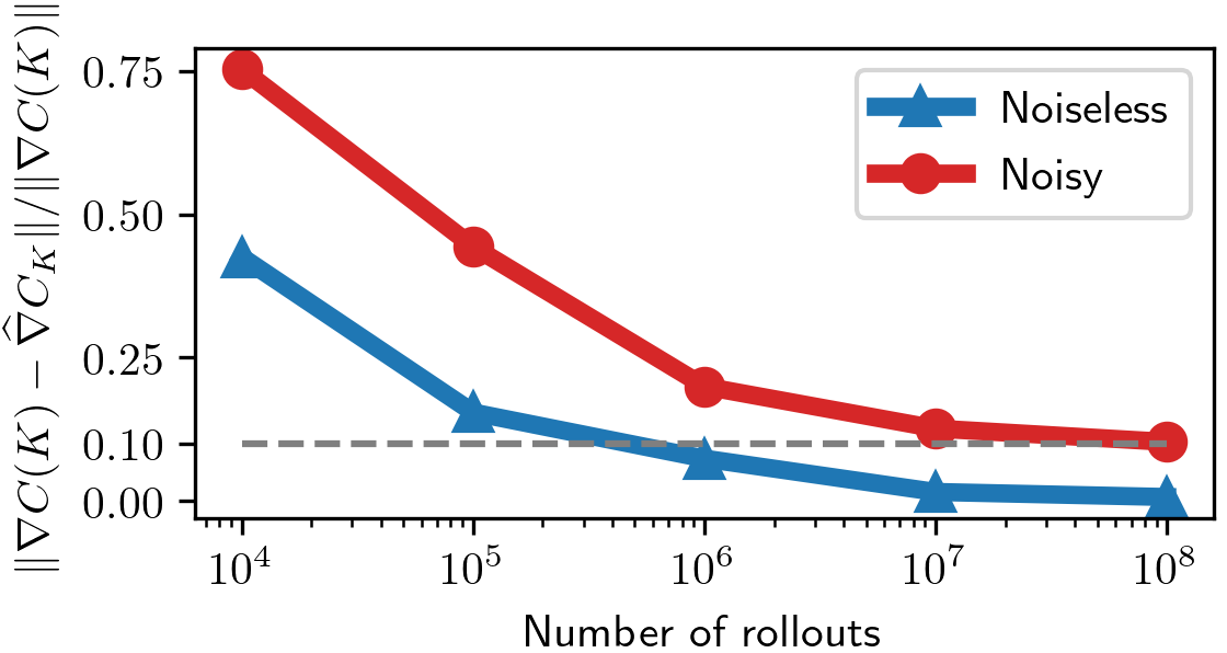
    Shows the increased difficulty of estimating the gradient from sample data in the presence of multiplicative noise.

All systems considered permitted a solution to the GARE (3). The bounds on the step size, number of rollouts, and rollout length given by the theoretical analysis can be rather conservative. For practicality, we selected the constant step size, number of rollouts, rollout length, and exploration radius according to a grid search over reasonable values. Additionally, we investigated the use of backtracking line search to adaptively select the step size; see e.g. [11]. Throughout the simulations, we computed the baseline optimal cost C⁡(K∗)C(K^{*}) by solving the GARE (3) to high precision via value iteration. Python code which implements the algorithms and generates the figures reported in this work can be found in the GitHub repository at https://github.com/TSummersLab/polgrad-multinoise/. The code was run on a desktop PC with a quad-core Intel i7 6700K 4.0GHz CPU, 16GB RAM; no GPU computing was utilized.

6.1. Importance of Accounting for Multiplicative Noise

We first considered an open-loop mean-square unstable system with four states and one input representing an active two-mass suspension converted from continuous to discrete time using a standard bilinear transformation, with parameters:

A=[+0.261+0.315+0.093−0.008−2.955+0.261+0.373−0.033+1.019+0.255−0.853+0.011−3.170−0.793−4.902−0.146],B=[0.1330.5320.1612.165],Q=I4,R=I1,\displaystyle A=\begin{bmatrix}+0.261&+0.315&+0.093&-0.008\\ -2.955&+0.261&+0.373&-0.033\\ +1.019&+0.255&-0.853&+0.011\\ -3.170&-0.793&-4.902&-0.146\end{bmatrix},\quad B=\begin{bmatrix}0.133\\ 0.532\\ 0.161\\ 2.165\end{bmatrix},\quad Q=I_{4},\quad R=I_{1},
[Ai]y,z={1​ if ​z=i,0​ otherwise,​B1=𝟏4×1,{αi}={0.017,0.017,0.017,0.017},β1=0.035.\displaystyle[A_{i}]_{y,z}=\begin{cases}1\text{ if }z=i,\\ 0\text{ otherwise,}\end{cases}B_{1}=\mathbf{1}_{4\times 1},\quad\{\alpha_{i}\}=\{0.017,0.017,0.017,0.017\},\quad\beta_{1}=0.035.

We performed model-based policy gradient descent; at each iteration gradients were calculated by solving generalized Lyapunov equations (9) and (11) using the problem data. The gains KmK_{m} and KℓK_{\ell} represent iterates during optimization of (“training” on) the LQRm and LQR cost (with the multiplicative noise variances set to zero), respectively. We performed the optimization starting from the same feasible initial gain, which was generated by perturbing the exact solution of the generalized algebraic Riccati equation such that the LQRm cost under the initial control was approximately 10 times that of the optimal control. The step size was chosen via backtracking line search. The optimization stopped once the Frobenius norm of the gradient fell below a small threshold. The plot in Fig. 1 shows the “testing” cost of the gains at each iteration evaluated on the LQRm cost (with multiplicative noise). From this figure, it is clear that KmK_{m} minimized the LQRm as desired. When there was high multiplicative noise, the noise-ignorant controller KℓK_{\ell} actually destabilized the system in the mean-square sense; this can be seen as the LQRm cost exploded upwards to infinity after iteration 10. In this sense, the multiplicative noise-aware optimization is generally safer and more robust than noise-ignorant optimization, and in examples like this is actually necessary for mean-square stabilization.

Refer to caption
(a) LQRm cost.
Refer to caption
(b) LQR cost.
Figure 1. Relative cost error C⁡(K)−C⁡(K∗)C⁡(K∗)\frac{C(K)-C(K^{*})}{C(K^{*})} vs. iteration during policy gradient descent on the 4-state, 1-input suspension example system.

6.2. Policy Gradient Methods Applied to a Network

Many practical networked systems can be approximated by diffusion dynamics with losses and stochastic diffusion constants (edge weights) between nodes; examples include heat flow through uninsulated pipes, hydraulic flow through leaky pipes, information flow between processors with packet loss, electrical power flow between generators with resistant electrical power lines, etc. A derivation of the discrete-time dynamics of this system is given in [57]. We considered a particular 4-state, 4-input system and open-loop mean-square stable with the following parameters:

A\displaystyle A =[0.7950.0500.1000.0500.0500.8450.0500.0500.1000.0500.6950.1500.0500.0500.1500.745],B=Q=R=Σ0=I4,\displaystyle=\begin{bmatrix}0.795&0.050&0.100&0.050\\ 0.050&0.845&0.050&0.050\\ 0.100&0.050&0.695&0.150\\ 0.050&0.050&0.150&0.745\end{bmatrix},\quad B=Q=R=\Sigma_{0}=I_{4},
{αi}\displaystyle\{\alpha_{i}\} ={0.005,0.015,0.010,0.015,0.005,0.020},{βj}={0.050,0.150,0.050,0.100},\displaystyle=\{0.005,0.015,0.010,0.015,0.005,0.020\},\quad\{\beta_{j}\}=\{0.050,0.150,0.050,0.100\},
[Ai]y,z\displaystyle[A_{i}]_{y,z} ={+1 if {ci=y&di=y} or {ci=z&di=z},−1 if {ci=z&di=y} or {ci=y&di=z},0​ otherwise, [Bj]y,z={+1​ if ​j=y=z,0​ otherwise. \displaystyle=\begin{cases}+1\text{ if }\{c_{i}\!=\!y\ \&\ d_{i}\!=\!y\}\text{ or }\{c_{i}\!=\!z\ \&\ d_{i}\!=\!z\},\\ -1\text{ if }\{c_{i}\!=\!z\ \&\ d_{i}\!=\!y\}\text{ or }\{c_{i}\!=\!y\ \&\ d_{i}\!=\!z\},\\ 0\text{ otherwise, }\end{cases}\quad[B_{j}]_{y,z}=\begin{cases}+1\text{ if }j=y=z,\\ 0\text{ otherwise. }\end{cases}
{(ci,di)}\displaystyle\{(c_{i},d_{i})\} ={(1,2),(1,3),(1,4),(2,3),(2,4),(3,4)}.\displaystyle=\{(1,2),(1,3),(1,4),(2,3),(2,4),(3,4)\}.

This system is open-loop mean-square stable, so we initialized the gains to all zeros for each trial. We performed policy optimization using the model-free gradient, and the model-based gradient, model-based natural gradient, and model-based Gauss-Newton step directions on 20 unique problem instances using two step size schemes:
Backtracking line search: Step sizes η\eta were chosen adaptively at each iteration by backtracking line search with parameters α=0.01\alpha=0.01, β=0.5\beta=0.5 (see [11] for a description), except for Gauss-Newton which used the optimal constant step-size of 1/21/2. Model-free gradients and costs were estimated with 100,000 rollouts per iteration. We ran a fixed number, 20, of iterations chosen such that the final cost using model-free gradient descent was no more than 5%5\% worse than optimal.
Constant step size: Step sizes were set to constants chosen as large as possible without observing infeasibility or divergence, which on this problem instance was η=5×10⁻⁵\eta=5\times 10^{-5} for gradient, η=2×10⁻⁴\eta=2\times 10^{-4} for natural gradient, and η=1/2\eta=1/2 for Gauss-Newton step directions. Model-free gradients were estimated with 1,000 rollouts per iteration. We ran a fixed number, 20,000, of iterations chosen such that convergence was achieved with all step directions.

In both cases sample gains were chosen for model-free gradient estimation with exploration radius r=0.1r\!=\!0.1 and the rollout length was set to ℓ=20\ell\!=\!20. The plots in Fig. 2 show the relative cost over the iterations; for the model-free gradient descent, the bold centerline is the mean of all trials and the shaded region is between the 10th and 90th percentile of all trials. Using backtracking line search, it is evident that in terms of convergence the Gauss-Newton step was extremely fast, and both the natural gradient and model-based gradient were slightly slower, but still quite fast. The model-free policy gradient converged to a reasonable neighborhood of the minimum cost quickly, but stagnated with further iterations; this is a consequence of the inherent gradient and cost estimation errors that arise due to random sampling and the multiplicative noise. Using constant stepsizes, we were forced to take small steps due to the steepness of the cost function near the initial gains, slowing overall convergence using the gradient and natural gradient methods. Here we observed that Gauss-Newton again converged most quickly, followed by natural gradient and lastly the gradient methods. The smaller step size also allowed us to use far fewer samples in the model-free setting, where we observed somewhat faster initial cost decrease with eventual stagnation around 10−210^{-2}, or 1%, relative error, which represents excellent control performance. All algorithms exhibited convergence to the optimum, confirming the asserted theoretical claims.

Refer to caption
(a) Backtracking line search.
Refer to caption
(b) Constant step sizes.
Figure 2. Relative cost error C⁡(K)−C⁡(K∗)C⁡(K∗)\frac{C(K)-C(K^{*})}{C(K^{*})} vs. iteration during policy gradient methods on a 4-state, 4-input lossy diffusion network with multiplicative noise using a) backtracking line search and b) constant step sizes.

6.3. Gradient Estimation

Multiplicative noise can significantly increase the variance and sample complexity of cost gradient estimates relative to the noiseless case, which is novelly reflected in the theoretical analysis for the number of rollouts and rollout length. To demonstrate this empirically, we evaluated the relative gradient estimation error vs. number of rollouts for the system

xt+1=([0.80.10.10.8]+δt​[0110]+[10]​K)​xt\displaystyle{x_{t+1}=\left(\begin{bmatrix}0.8&0.1\\ 0.1&0.8\end{bmatrix}+\delta_{t}\begin{bmatrix}0&1\\ 1&0\end{bmatrix}+\begin{bmatrix}1\\ 0\end{bmatrix}K\right)x_{t}} (121)

with K=0,Q=Σ0=I2,R=1K=0,Q=\Sigma_{0}=I_{2},R=1, δt∼𝒩⁡(0,0.1)\delta_{t}\sim\mathcal{N}(0,0.1), rollout length l=40l=40, exploration radius r=0.2r=0.2, averaged over 10 gradient estimates. The results are plotted in Figure 3. To achieve the same gradient estimate error of 10%10\%, the system with multiplicative noise required 200×200\times the number of rollout samples (10810^{8}) as when there was no noise (5×1055\times 10^{5}).

Refer to caption
Figure 3. Relative gradient estimation error vs. number of rollouts for (121).

7. Conclusions

We have shown that policy gradient methods in both model-based and model-free settings give global convergence to the globally optimal policy for LQR systems with multiplicative noise. These techniques are directly applicable for the design of robust controllers of uncertain systems and serve as a benchmark for data-driven control design. Our ongoing work is exploring ways of mitigating the relative sample inefficiency of model-free policy gradient methods by leveraging the special structure of LQR models and Nesterov-type acceleration, and exploring alternative system identification and adaptive control approaches. We are also investigating other methods of building robustness through ℋ∞\mathcal{H}_{\infty} and dynamic game approaches. Another extension relevant to networked control systems is enforcing sparse structure constraints on the gain matrix via projected policy gradient as suggested in [14].

Appendix A Standard matrix expressions

Before proceeding with the proof of the main results of this study, we first review several basic expressions that will be used later throughout the section. In this section we let AA, BB, CC, MiM_{i} be generic matrices ∈ℝn×m\in\mathds{R}^{n\times m}, aa, bb be generic vectors, and ss be a generic scalar.

Spectral norm:

We denote the matrix spectral norm as ‖A‖=σmax​(A)\|A\|=\sigma_{\text{max}}(A) which clearly satisfies

‖A‖=σmax​(A)≥σmin​(A).\|A\|=\sigma_{\text{max}}(A)\geq\sigma_{\min}(A). (122)
Frobenius norm:

We denote the matrix Frobenius norm as ‖A‖F\|A\|_{F} whose square satisfies

‖A‖F2=Tr⁡(AT​A).\|A\|_{F}^{2}=\Tr(A^{T}A). (123)
Frobenius norm ≥\geq spectral norm:

For any matrix AA the Frobenius norm is greater than or equal to the spectral norm:

‖A‖F≥‖A‖.\|A\|_{F}\geq\|A\|. (124)
Inverse of spectral norm inequality:
‖A−1‖≥‖A‖−1.\|A^{-1}\|\geq\|A\|^{-1}. (125)
Invariance of trace under cyclic permutation:
Tr⁡(∏i=1nMi)=Tr⁡(Mn​∏i=1n−1Mi).\Tr\left(\prod_{i=1}^{n}M_{i}\right)=\Tr\left(M_{n}\prod_{i=1}^{n-1}M_{i}\right). (126)
Invariance of trace under arbitrary permutation for a product of three matrices:
Tr⁡(A​B​C)=Tr⁡(B​C​A)=Tr⁡(C​A​B)=Tr⁡(A​C​B)=Tr⁡(B​A​C)=Tr⁡(C​B​A).\Tr(ABC)=\Tr(BCA)=\Tr(CAB)=\Tr(ACB)=\Tr(BAC)=\Tr(CBA). (127)
Scalar trace equivalence:
s=Tr⁡(s).s=\Tr(s). (128)
Trace-spectral norm inequalities:
|Tr⁡(AT​B)|≤‖AT‖|Tr⁡(B)|=‖A‖​|Tr⁡(B)|.|\Tr(A^{T}B)|\leq\|A^{T}\||\Tr(B)|=\|A\||\Tr(B)|. (129)

If A∈ℝn×nA\in\mathds{R}^{n\times n}

|Tr⁡(A)|≤n​‖A‖|\Tr(A)|\leq n\|A\| (130)

and if A⪰0A\succeq 0

Tr⁡(A)≥‖A‖.\Tr(A)\geq\|A\|. (131)
Sub-multiplicativity of spectral norm:
‖A​B‖≤‖A‖​‖B‖.\|AB\|\leq\|A\|\|B\|. (132)
Positive semidefinite matrix inequality:

Suppose A⪰0A\succeq 0 and B⪰0B\succeq 0. Then

A+B⪰A​ and ​A+B⪰B.A+B\succeq A\text{ \ and \ }A+B\succeq B. (133)
Vector self outer product positive semidefiniteness:
a​aT⪰0aa^{T}\succeq 0 (134)

since bT​a​aT​b=(aT​b)T​(aT​b)≥0​ for any ​bb^{T}aa^{T}b=(a^{T}b)^{T}(a^{T}b)\geq 0\text{ for any }b.

Singular value inequality for positive semidefinite matrices:

Suppose A⪰0A\succeq 0 and B⪰0B\succeq 0 and A⪰BA\succeq B. Then

σmin​(A)≥σmin​(B).\sigma_{\min}(A)\geq\sigma_{\min}(B). (135)
Weyl’s Inequality for singular values:

Suppose B=A+CB=A+C. Let singular values of AA, BB, and CC be

σ1​(A)≥σ2​(A)≥…≥σr​(A)≥0\displaystyle\sigma_{1}(A)\geq\sigma_{2}(A)\geq\ldots\geq\sigma_{r}(A)\geq 0
σ1​(B)≥σ2​(B)≥…≥σr​(B)≥0\displaystyle\sigma_{1}(B)\geq\sigma_{2}(B)\geq\ldots\geq\sigma_{r}(B)\geq 0
σ1​(C)≥σ2​(C)≥…≥σr​(C)≥0\displaystyle\sigma_{1}(C)\geq\sigma_{2}(C)\geq\ldots\geq\sigma_{r}(C)\geq 0

where r=min⁡{m,n}r=\min\{m,n\}. Then we have

σi+j−1​(B)≤σi​(A)+σj​(C)​∀i∈{1,2,…​r},j∈{1,2,…​r},i+j−1∈{1,2,…​r}.\displaystyle\sigma_{i+j-1}(B)\leq\sigma_{i}(A)+\sigma_{j}(C)\ \forall\ i\in\{1,2,\ldots r\},j\in\{1,2,\ldots r\},i+j-1\in\{1,2,\ldots r\}. (136)

Consequently, we have

‖B‖≤‖A‖+‖C‖\|B\|\leq\|A\|+\|C\| (137)

and

σmin​(B)≥σmin​(A)−‖C‖.\sigma_{\min}(B)\geq\sigma_{\min}(A)-\|C\|. (138)
Vector Bernstein inequality:

Suppose a^=∑ia^i,\hat{a}=\sum_{i}\hat{a}_{i}, where a^i\hat{a}_{i} are independent random vectors of dimension nn. Let 𝔼⁡[a^]=a\mathbb{E}[\hat{a}]=a , and the variance σ2=𝔼⁡[∑i‖a^i‖2]\sigma^{2}=\mathbb{E}\left[\sum_{i}\left\|\hat{a}_{i}\right\|^{2}\right]. If every a^i\hat{a}_{i} has norm ‖a^i‖≤s\left\|\hat{a}_{i}\right\|\leq s then with high probability we have

‖a^−a‖≤𝒪⁡(s​log⁡n+σ2​log⁡n).\displaystyle\|\hat{a}-a\|\leq\mathcal{O}\left(s\log n+\sqrt{\sigma^{2}\log n}\right). (139)

This is the same inequality given in [19]. See [50] for the exact scale constants and a proof.

Appendix B Model-based policy gradient descent

The proof of convergence using gradient descent proceeds by establishing several technical lemmas, bounding the infinite-horizon covariance ΣK\Sigma_{K}, then using that bound to limit the step size, and finally obtaining a one-step bound on gradient descent progress and applying it inductively at each successive step. We begin with a bound on the induced operator norm of 𝒯K\mathcal{T}_{K}:

Lemma B.1.

(𝒯K\mathcal{T}_{K} norm bound) The following bound holds for any mean-square stabilizing KK:

‖𝒯K‖≔sup𝑋​‖𝒯K​(X)‖‖X‖≤C⁡(K)σ¯​(Σ0)​σ¯​(Q).\displaystyle\|\mathcal{T}_{K}\|\coloneqq\underset{X}{\text{sup}}\frac{\|\mathcal{T}_{K}(X)\|}{\|X\|}\leq\frac{C(K)}{{\underline{\sigma}(\Sigma_{0})}\underline{\sigma}(Q)}. (140)
Proof.

The proof follows that given in [19] using our definition of 𝒯K\mathcal{T}_{K}. ∎

Lemma B.2.

(ℱK\mathcal{F}_{K} perturbation) Consider a pair of mean-square stabilizing gain matrices KK and K′K{{}^{\prime}}. The following ℱK\mathcal{F}_{K} perturbation bound holds:

∥ℱK′−ℱK∥\displaystyle\|\mathcal{F}_{K{{}^{\prime}}}-\mathcal{F}_{K}\| ≤2​‖A+B​K​‖‖B‖‖​Δ​‖+hB‖​B‖​‖Δ‖2\displaystyle\leq 2\|A+BK\|\|B\|\|\Delta\|+h_{B}\|B\|\|\Delta\|^{2} (141)
where hB\displaystyle\text{where }\quad h_{B} ≔‖B‖−1​(‖B‖2+∑j=1qβj​‖Bj‖2).\displaystyle\coloneqq{\|B\|}^{-1}\big(\|B\|^{2}+\sum_{j=1}^{q}\beta_{j}\|B_{j}\|^{2}\big). (142)
Proof.

Let Δ′=−Δ\Delta^{\prime}=-\Delta. For any matrix XX we have

(ℱK−ℱK′)(X)\displaystyle(\mathcal{F}_{K}-\mathcal{F}_{K{{}^{\prime}}})(X) =𝔼δ,γ[A~KXA~K⊺−A~K′XA~K′⊺]\displaystyle=\underset{\delta,\gamma}{\mathbb{E}}\left[\widetilde{A}_{K}X\widetilde{A}_{K}^{\intercal}-\widetilde{A}_{K{{}^{\prime}}}X\widetilde{A}_{K{{}^{\prime}}}^{\intercal}\right] (143)
=𝔼δ,γ​[A~K​X​(B~​Δ′)⊺+(B~​Δ′)​X​A~K⊺−(B~​Δ′)​X​(B~​Δ′)⊺]\displaystyle=\underset{\delta,\gamma}{\mathbb{E}}\left[\widetilde{A}_{K}X(\widetilde{B}\Delta^{\prime})^{\intercal}+(\widetilde{B}\Delta^{\prime})X\widetilde{A}_{K}^{\intercal}-(\widetilde{B}\Delta^{\prime})X(\widetilde{B}\Delta^{\prime})^{\intercal}\right] (144)
=AK​X​(B​Δ′)⊺+(B​Δ′)​X​AK⊺−𝔼γt​j​[(B~​Δ′)​X​(B~​Δ′)⊺]\displaystyle=A_{K}X({B}\Delta^{\prime})^{\intercal}+({B}\Delta^{\prime})XA_{K}^{\intercal}-\underset{\gamma_{tj}}{\mathbb{E}}\left[(\widetilde{B}\Delta^{\prime})X(\widetilde{B}\Delta^{\prime})^{\intercal}\right] (145)
=AK​X​(B​Δ′)⊺+(B​Δ′)​X​AK⊺−(B​Δ′)​X​(B​Δ′)⊺−∑j=1qβj​(Bj​Δ′)​X​(Bj​Δ′)⊺.\displaystyle=A_{K}X({B}\Delta^{\prime})^{\intercal}+({B}\Delta^{\prime})XA_{K}^{\intercal}-(B\Delta^{\prime})X(B\Delta^{\prime})^{\intercal}-\sum_{j=1}^{q}\beta_{j}(B_{j}\Delta^{\prime})X(B_{j}\Delta^{\prime})^{\intercal}. (146)

The operator norm ∥ℱK′−ℱK∥\|\mathcal{F}_{K{{}^{\prime}}}-\mathcal{F}_{K}\| is

∥ℱK′−ℱK∥=∥ℱK−ℱK′∥=sup𝑋∥(ℱK−ℱK′)(X)∥‖X‖\displaystyle\|\mathcal{F}_{K{{}^{\prime}}}-\mathcal{F}_{K}\|=\|\mathcal{F}_{K}-\mathcal{F}_{K{{}^{\prime}}}\|=\underset{X}{\text{sup}}\ \frac{\|(\mathcal{F}_{K}-\mathcal{F}_{K{{}^{\prime}}})(X)\|}{\|X\|} (147)

Applying submultiplicativity of spectral norm to (146) and noting that ‖Δ′‖=‖Δ‖\|\Delta^{\prime}\|=\|\Delta\| completes the proof. ∎

Lemma B.3 (𝒯K\mathcal{T}_{K} perturbation).

If KK and K′K{{}^{\prime}} are mean-square stabilizing and ∥𝒯K∥∥ℱK′−ℱK∥≤12\|\mathcal{T}_{K}\|\|\mathcal{F}_{K{{}^{\prime}}}-\mathcal{F}_{K}\|\leq\frac{1}{2} then

∥(𝒯K′−𝒯K)(Σ)∥\displaystyle\|(\mathcal{T}_{K{{}^{\prime}}}-\mathcal{T}_{K})(\Sigma)\| ≤2∥𝒯K∥∥ℱK′−ℱK∥∥𝒯K(Σ)∥\displaystyle\leq 2\|\mathcal{T}_{K}\|\|\mathcal{F}_{K{{}^{\prime}}}-\mathcal{F}_{K}\|\|\mathcal{T}_{K}(\Sigma)\| (148)
≤2∥𝒯K∥2∥ℱK′−ℱK∥∥Σ∥.\displaystyle\leq 2\|\mathcal{T}_{K}\|^{2}\|\mathcal{F}_{K{{}^{\prime}}}-\mathcal{F}_{K}\|\|\Sigma\|. (149)
Proof.

The proof follows [19] using our modified definitions of 𝒯K\mathcal{T}_{K} and ℱK\mathcal{F}_{K}. ∎

Lemma B.4 (ΣK\Sigma_{K} trace bound).

If ρ⁡(ℱK)<1\rho(\mathcal{F}_{K})<1 then

Tr⁡(ΣK)≥σ¯​(Σ0)1−ρ⁡(ℱK).\displaystyle\Tr\left(\Sigma_{K}\right)\geq\frac{{\underline{\sigma}(\Sigma_{0})}}{1-\rho(\mathcal{F}_{K})}. (150)
Proof.

We have by (17) that

Tr⁡(ΣK)\displaystyle\Tr(\Sigma_{K}) =Tr⁡(𝒯K​(Σ0))=∑t=0∞Tr⁡(ℱKt​(Σ0)).\displaystyle=\Tr(\mathcal{T}_{K}(\Sigma_{0}))=\sum_{t=0}^{\infty}\Tr({\mathcal{F}^{t}_{K}(\Sigma_{0})}). (151)

Since Σ0⪰σ¯​(Σ0)​I\Sigma_{0}\succeq{\underline{\sigma}(\Sigma_{0})}I we know the tt​ht^{th} term satisfies the inequality ℱKt​(Σ0)≥σ¯​(Σ0)​ℱKt​(I),{\mathcal{F}^{t}_{K}(\Sigma_{0})}\geq{\underline{\sigma}(\Sigma_{0})}{\mathcal{F}^{t}_{K}(I)}, so we have

Tr⁡(ΣK)≥σ¯​(Σ0)​∑t=0∞Tr⁡(ℱKt​(I)).\displaystyle\Tr(\Sigma_{K})\geq{\underline{\sigma}(\Sigma_{0})}\sum_{t=0}^{\infty}\Tr({\mathcal{F}^{t}_{K}(I)}). (152)

We have a generic inequality for a sum of nn matrices MiM_{i}:

Tr⁡[∑inMi​Mi⊺]=∑inTr⁡[Mi​Mi⊺]=∑in‖Mi‖F2=∑in‖Mi⊗Mi‖F≥‖∑inMi⊗Mi‖F\displaystyle\Tr\left[\sum_{i}^{n}M_{i}M_{i}^{\intercal}\right]=\sum_{i}^{n}\Tr\left[M_{i}M_{i}^{\intercal}\right]=\sum_{i}^{n}\left\|M_{i}\right\|_{F}^{2}=\sum_{i}^{n}\left\|M_{i}\otimes M_{i}\right\|_{F}\geq\left\|\sum_{i}^{n}M_{i}\otimes M_{i}\right\|_{F}

where the last step is due to the triangle inequality. Recalling the definitions of ℱKt​(I)\mathcal{F}^{t}_{K}(I) and ℱKt\mathcal{F}^{t}_{K} we see they are of the form of the LHS and RHS in (B) with all terms matched between ℱKt​(I)\mathcal{F}^{t}_{K}(I) and ℱKt\mathcal{F}^{t}_{K} so that the inequality in (B) holds; this can be seen by starting with t=1t=1 and incrementing tt up by 11 which will give (1+p+q)t(1+p+q)^{t} terms which are all matched. Thus,

Tr⁡[ℱKt​(I)]≥‖ℱKt‖F≥ρ​(ℱK)t.\displaystyle\Tr[\mathcal{F}^{t}_{K}(I)]\geq\|\mathcal{F}^{t}_{K}\|_{F}\geq\rho(\mathcal{F}_{K})^{t}. (153)

Continuing from (152) we have

Tr⁡(ΣK)≥σ¯​(Σ0)​∑t=0∞ρ​(ℱK)t.\displaystyle\Tr(\Sigma_{K})\geq{\underline{\sigma}(\Sigma_{0})}\sum_{t=0}^{\infty}\rho(\mathcal{F}_{K})^{t}. (154)

By hypothesis ρ⁡(ℱK)<1\rho(\mathcal{F}_{K})<1, and taking the sum of the geometric series completes the proof. ∎

Lemma B.5 (ΣK\Sigma_{K} perturbation).

If KK is mean-square stabilizing and ‖Δ‖≤hΔ​(K)\|\Delta\|\leq h_{\Delta}(K) where hΔ​(K)h_{\Delta}(K) is the polynomial

hΔ​(K)\displaystyle h_{\Delta}(K) ≔σ¯​(Q)​σ¯​(Σ0)4​hB​C​(K)​(‖AK‖+1),\displaystyle\coloneqq\frac{\underline{\sigma}(Q){\underline{\sigma}(\Sigma_{0})}}{4h_{B}C(K)\left(\|A_{K}\|+1\right)}, (155)

then the associated state covariance matrices satisfy

‖ΣK′−ΣK‖≤4​(C⁡(K)σ¯​(Q))2​‖B‖​(‖AK‖+1)σ¯​(Σ0)​‖Δ‖≤C⁡(K)σ¯​(Q).\displaystyle\|\Sigma_{K^{\prime}}\!-\!\Sigma_{K}\|\leq 4\left(\frac{C(K)}{\underline{\sigma}(Q)}\right)^{2}\frac{\|B\|(\|A_{K}\|+1)}{{\underline{\sigma}(\Sigma_{0})}}\|\Delta\|\leq\frac{C(K)}{\underline{\sigma}(Q)}.
Proof.

First we show that KK is mean-square stabilizing and ‖Δ‖≤hΔ​(K)\|\Delta\|\leq h_{\Delta}(K) then K′K{{}^{\prime}} is also mean-square stabilizing. This follows from an analogous argument in [19] by characterizing mean-square stability in terms of ρ⁡(ℱK)\rho(\mathcal{F}_{K}) rather than ρ⁡(AK)\rho(A_{K}) and using Lemma B.4. Let K′′K^{\prime\prime} be distinct from KK with ρ⁡(ℱK′′)<1\rho(\mathcal{F}_{K^{\prime\prime}})<1 and ‖K′′−K‖≤hΔ\|K^{\prime\prime}-K\|\leq h_{\Delta}. We have

|Tr⁡(ΣK′′−ΣK)|≤n​‖ΣK′′−ΣK‖.\displaystyle|\Tr(\Sigma_{K^{\prime\prime}}-\Sigma_{K})|\leq n\|\Sigma_{K^{\prime\prime}}-\Sigma_{K}\|. (156)

Since KK and K′′K^{\prime\prime} are mean-square stabilizing Lemma B.5 holds so we have

|Tr⁡(ΣK′′−ΣK)|≤n​C⁡(K)σmin​(Q)⇒Tr⁡(ΣK′′)≤Γ,\displaystyle|\Tr(\Sigma_{K^{\prime\prime}}-\Sigma_{K})|\leq n\frac{C(K)}{\sigma_{\min}(Q)}\Rightarrow\Tr(\Sigma_{K^{\prime\prime}})\leq\Gamma, (157)

where we define

Γ≔Tr⁡(ΣK)+n​C⁡(K)σmin​(Q),ϵ=σmin​(Σ0)2​Γ.\displaystyle\Gamma\coloneqq\Tr(\Sigma_{K})+n\frac{C(K)}{\sigma_{\min}(Q)},\quad\epsilon=\frac{\sigma_{\min}(\Sigma_{0})}{2\Gamma}. (158)

Using Lemma B.4 we have

Tr⁡(ΣK)≥σmin​(Σ0)1−ρ⁡(ℱK)=2​ϵ​Γ1−ρ⁡(ℱK)\displaystyle\Tr\left(\Sigma_{K}\right)\geq\frac{{\sigma_{\min}(\Sigma_{0})}}{1-\rho(\mathcal{F}_{K})}=\frac{{2\epsilon\Gamma}}{1-\rho(\mathcal{F}_{K})} (159)

Rearranging and substituting for Γ\Gamma,

ρ⁡(ℱK)≤1−2​ϵ​ΓTr⁡(ΣK)\displaystyle\rho(\mathcal{F}_{K})\leq 1-\frac{2\epsilon\Gamma}{\Tr(\Sigma_{K})} =1−2​ϵ​(Tr⁡(ΣK)+n​C⁡(K)σmin​(Q))Tr⁡(ΣK)\displaystyle=1-\frac{2\epsilon\left(\Tr(\Sigma_{K})+n\frac{C(K)}{\sigma_{\min}(Q)}\right)}{\Tr(\Sigma_{K})}
=1−2​ϵ​(1+n​C​(K)σmin​(Q)​Tr⁡(ΣK))\displaystyle=1-2\epsilon\left(1+\frac{nC(K)}{\sigma_{\min}(Q)\Tr(\Sigma_{K})}\right) (160)
<1−2​ϵ<1−ϵ.\displaystyle<1-2\epsilon<1-\epsilon. (161)

Now we construct the proof by contradiction. Suppose there is a K′K^{\prime} with ρ⁡(ℱK′)>1\rho(\mathcal{F}_{K^{\prime}})>1 satisfying the perturbation restriction

‖K′−K‖≤hΔ.\displaystyle\|K^{\prime}-K\|\leq h_{\Delta}. (162)

Since spectral radius is a continuous function (see [52]) there must be a point K′′′K^{\prime\prime\prime} on the path between KK and K′K^{\prime} such that ρ⁡(ℱK′′′)=1−ϵ<1\rho(\mathcal{F}_{K^{\prime\prime\prime}})=1-\epsilon<1. Since KK and K′′′K^{\prime\prime\prime} are mean-square stabilizing Lemma B.5 holds so we have

|Tr⁡(ΣK′′′−ΣK)|≤n​C⁡(K)σmin​(Q),\displaystyle|\Tr(\Sigma_{K^{\prime\prime\prime}}-\Sigma_{K})|\leq n\frac{C(K)}{\sigma_{\min}(Q)}, (163)

and rearranging

Tr⁡(ΣK′′′)≤Tr⁡(ΣK)+n​C⁡(K)σmin​(Q)=Γ.\displaystyle\Tr(\Sigma_{K^{\prime\prime\prime}})\leq\Tr(\Sigma_{K})+n\frac{C(K)}{\sigma_{\min}(Q)}=\Gamma. (164)

However since K′′′K^{\prime\prime\prime} is mean-square stabilizing Lemma B.4 holds so we have

Tr⁡(ΣK′′′)≥σmin​(Σ0)1−ρ⁡(ℱK′′′)=2​ϵ​Γ1−(1−ϵ)=2​Γ\displaystyle\Tr\left(\Sigma_{K^{\prime\prime\prime}}\right)\geq\frac{{\sigma_{\min}(\Sigma_{0})}}{1-\rho(\mathcal{F}_{K^{\prime\prime\prime}})}=\frac{{2\epsilon\Gamma}}{1-(1-\epsilon)}=2\Gamma (165)

which is a contradiction. Therefore no such mean-square unstable K′K^{\prime} satisfying the hypothesized perturbation restriction can exist, completing the first part of the proof.

The rest of the proof follows [19] by using the condition on ‖Δ‖\|\Delta\|, ‖ΣK‖≥σ¯​(Σ0){\|\Sigma_{K}\|\geq{\underline{\sigma}(\Sigma_{0})}}, and Lemmas 3.7, B.1, and B.3. The condition on ‖Δ‖\|\Delta\| directly implies

hB​‖Δ‖\displaystyle h_{B}\|\Delta\| ≤σ¯​(Q)​σ¯​(Σ0)4​C​(K)​(‖AK‖+1)≤σ¯​(Q)​σ¯​(Σ0)4​C​(K)≤14.\displaystyle\leq\frac{\underline{\sigma}(Q){\underline{\sigma}(\Sigma_{0})}}{4C(K)\left(\|A_{K}\|+1\right)}\leq\frac{\underline{\sigma}(Q){\underline{\sigma}(\Sigma_{0})}}{4C(K)}\leq\frac{1}{4}. (166)

where the last step is due to the combination of Lemma 3.7 with ‖ΣK‖≥σ¯​(Σ0){\|\Sigma_{K}\|\geq{\underline{\sigma}(\Sigma_{0})}}. By Lemma B.2 we have

∥ℱK′−ℱK∥\displaystyle\|\mathcal{F}_{K{{}^{\prime}}}-\mathcal{F}_{K}\| ≤2​‖B‖​‖Δ‖​(‖A+B​K‖+‖Δ‖​hB/2)\displaystyle\leq 2\|B\|\|\Delta\|\big(\|A+BK\|+\|\Delta\|h_{B}/2\big) (167)
≤2​‖B‖​‖Δ‖​(‖A+B​K‖+1/8)\displaystyle\leq 2\|B\|\|\Delta\|\big(\|A+BK\|+1/8\big) (168)
≤2​‖B‖​‖Δ‖​(‖A+B​K‖+1).\displaystyle\leq 2\|B\|\|\Delta\|\big(\|A+BK\|+1\big). (169)

Combining this with Lemma B.1 we have

∥TK∥∥ℱK′−ℱK∥≤(C⁡(K)σ¯​(Σ0)​σ¯​(Q))(2∥B∥∥Δ∥(∥AK∥+1)).\displaystyle\|T_{K}\|\|\mathcal{F}_{K{{}^{\prime}}}-\mathcal{F}_{K}\|\leq\left(\frac{C(K)}{{\underline{\sigma}(\Sigma_{0})}\underline{\sigma}(Q)}\right)\left(2\|B\|\|\Delta\|\left(\|A_{K}\|+1\right)\right). (170)

By the condition on ‖Δ‖\|\Delta\| we have

‖Δ‖\displaystyle\|\Delta\| ≤σ¯​(Q)​σ¯​(Σ0)4​C​(K)​‖B‖​(‖AK‖+1),\displaystyle\leq\frac{\underline{\sigma}(Q){\underline{\sigma}(\Sigma_{0})}}{4C(K)\|B\|\left(\|A_{K}\|+1\right)}, (171)

so

∥TK∥∥ℱK′−ℱK∥\displaystyle\|T_{K}\|\|\mathcal{F}_{K{{}^{\prime}}}-\mathcal{F}_{K}\| ≤12\displaystyle\leq\frac{1}{2} (172)

which allows us to use Lemma B.3 by which we have

∥(𝒯K−𝒯K)(Σ0)∥≤2∥𝒯K∥∥ℱK′−ℱK∥∥𝒯K(Σ0)∥≤(2​C​(K)σ¯​(Σ0)​σ¯​(Q))(2∥B∥∥Δ∥(∥AK∥+1))∥𝒯K(Σ0)∥\displaystyle\|(\mathcal{T}_{K}-\mathcal{T}_{K})(\Sigma_{0})\|\leq 2\|\mathcal{T}_{K}\|\|\mathcal{F}_{K{{}^{\prime}}}-\mathcal{F}_{K}\|\|\mathcal{T}_{K}(\Sigma_{0})\|\leq\left(\frac{2C(K)}{{\underline{\sigma}(\Sigma_{0})}\underline{\sigma}(Q)}\right)\left(2\|B\|\|\Delta\|\left(\|A_{K}\|+1\right)\right)\|\mathcal{T}_{K}(\Sigma_{0})\|

where the last step used (170). Using 𝒯K​(Σ0)=ΣK\mathcal{T}_{K}(\Sigma_{0})=\Sigma_{K} gives

∥ΣK′−ΣK∥≤(2​C​(K)σ¯​(Σ0)​σ¯​(Q))(2∥B∥∥Δ∥(∥AK∥+1))∥(ΣK)∥.\displaystyle\|\Sigma_{K{{}^{\prime}}}-\Sigma_{K}\|\leq\left(\frac{2C(K)}{{\underline{\sigma}(\Sigma_{0})}\underline{\sigma}(Q)}\right)\left(2\|B\|\|\Delta\|\left(\|A_{K}\|+1\right)\right)\|(\Sigma_{K})\|.

Using Lemma 3.7 completes the proof. ∎

Now we bound the one step progress of policy gradient where we allow the step size to depend explicitly on the current gain matrix iterate KsK_{s}.

Lemma B.6 (Gradient descent, one-step).

Using the policy gradient step update Ks+1=Ks−η∇C(Ks)K_{s+1}=K_{s}-\eta\nabla C(K_{s}) with step size

0<η≤116​min⁡{(σ¯​(Q)​σ¯​(Σ0)C⁡(K))2hB​‖∇C​(K)‖​(‖AK‖+1),σ¯​(Q)C⁡(K)​‖RK‖}\displaystyle 0<\eta\leq\frac{1}{16}\min\Bigg\{\frac{\left(\frac{\underline{\sigma}(Q){\underline{\sigma}(\Sigma_{0})}}{C(K)}\right)^{2}}{h_{B}\|\nabla C(K)\|(\|A_{K}\|+1)},\frac{\underline{\sigma}(Q)}{C(K)\|R_{K}\|}\Bigg\}

gives the one step progress bound

C⁡(Ks+1)−C⁡(K∗)C⁡(Ks)−C⁡(K∗)≤1−2​η​σ¯​(R)​σ¯​(Σ0)2‖ΣK∗‖.\displaystyle\frac{C(K_{s+1})-C(K^{*})}{C(K_{s})-C(K^{*})}\leq 1-2\eta\frac{\underline{\sigma}(R){\underline{\sigma}(\Sigma_{0})}^{2}}{\|\Sigma_{K^{*}}\|}. (173)
Proof.

The gradient update yields Δ=−2​η​EKs​ΣKs.\Delta=-2\eta E_{K_{s}}\Sigma_{K_{s}}. Putting this into Lemma 3.5 gives

C⁡(Ks+1)−C⁡(Ks)\displaystyle C(K_{s+1})-C(K_{s})
=2​Tr⁡[ΣKs+1​Δ⊺​EKs]+Tr⁡[ΣKs+1​Δ⊺​RKs​Δ]\displaystyle=2\Tr\big[\Sigma_{K_{s+1}}\Delta^{\intercal}E_{K_{s}}\big]+\Tr\big[\Sigma_{K_{s+1}}\Delta^{\intercal}R_{K_{s}}\Delta\big]
=−4​η​Tr⁡[ΣKs+1​ΣKs​EKs⊺​EKs]+4​η2​Tr⁡[ΣKs​ΣKs+1​ΣKs​EKs⊺​RKs​EKs]\displaystyle=-4\eta\Tr\big[\Sigma_{K_{s+1}}\Sigma_{K_{s}}E_{K_{s}}^{\intercal}E_{K_{s}}\big]+4\eta^{2}\Tr\big[\Sigma_{K_{s}}\Sigma_{K_{s+1}}\Sigma_{K_{s}}E_{K_{s}}^{\intercal}R_{K_{s}}E_{K_{s}}\big]
=−4​η​Tr⁡[ΣKs​ΣKs​EKs⊺​EKs]+4​η​Tr⁡[(−ΣKs+1+ΣKs)​ΣKs​EKs⊺​EKs]\displaystyle=-4\eta\Tr\big[\Sigma_{K_{s}}\Sigma_{K_{s}}E_{K_{s}}^{\intercal}E_{K_{s}}\big]+4\eta\Tr\big[(-\Sigma_{K_{s+1}}+\Sigma_{K_{s}})\Sigma_{K_{s}}E_{K_{s}}^{\intercal}E_{K_{s}}\big]
+4​η2​Tr⁡[ΣKs​ΣKs+1​ΣKs​EKs⊺​RKs​EKs]\displaystyle\quad+4\eta^{2}\Tr\big[\Sigma_{K_{s}}\Sigma_{K_{s+1}}\Sigma_{K_{s}}E_{K_{s}}^{\intercal}R_{K_{s}}E_{K_{s}}\big]
≤−4​η​Tr⁡[ΣKs​ΣKs​EKs⊺​EKs]+4​η​‖ΣKs+1−ΣKs‖​Tr⁡[ΣKs​EKs⊺​EKs]\displaystyle\leq-4\eta\Tr\big[\Sigma_{K_{s}}\Sigma_{K_{s}}E_{K_{s}}^{\intercal}E_{K_{s}}\big]+4\eta\|\Sigma_{K_{s+1}}-\Sigma_{K_{s}}\|\Tr\big[\Sigma_{K_{s}}E_{K_{s}}^{\intercal}E_{K_{s}}\big]
+4​η2​‖ΣKs+1‖​‖RKs‖​Tr⁡[ΣKs​ΣKs​EKs⊺​EKs]\displaystyle\quad+4\eta^{2}\|\Sigma_{K_{s+1}}\|\|R_{K_{s}}\|\Tr\big[\Sigma_{K_{s}}\Sigma_{K_{s}}E_{K_{s}}^{\intercal}E_{K_{s}}\big]
≤−4​η​Tr⁡[ΣKs​ΣKs​EKs⊺​EKs]+4​η​‖ΣKs+1−ΣKs‖σ¯​(ΣKs)​Tr⁡[ΣKs⊺​EKs⊺​EKs​ΣKs]\displaystyle\leq-4\eta\Tr\big[\Sigma_{K_{s}}\Sigma_{K_{s}}E_{K_{s}}^{\intercal}E_{K_{s}}\big]+4\eta\frac{\|\Sigma_{K_{s+1}}-\Sigma_{K_{s}}\|}{\underline{\sigma}(\Sigma_{K_{s}})}\Tr\big[\Sigma_{K_{s}}^{\intercal}E_{K_{s}}^{\intercal}E_{K_{s}}\Sigma_{K_{s}}\big]
+4​η2​‖ΣKs+1‖​‖RKs‖​Tr⁡[ΣKs​ΣKs​EKs⊺​EKs]\displaystyle\quad+4\eta^{2}\|\Sigma_{K_{s+1}}\|\|R_{K_{s}}\|\Tr\big[\Sigma_{K_{s}}\Sigma_{K_{s}}E_{K_{s}}^{\intercal}E_{K_{s}}\big]
=−4η(1−‖ΣKs+1−ΣKs‖σ¯​(ΣKs)−η∥ΣKs+1∥∥RKs∥)×Tr[ΣKs⊺EKs⊺EKsΣKs]\displaystyle=-4\eta\bigg(1-\frac{\|\Sigma_{K_{s+1}}-\Sigma_{K_{s}}\|}{\underline{\sigma}(\Sigma_{K_{s}})}-\eta\|\Sigma_{K_{s+1}}\|\|R_{K_{s}}\|\bigg)\times\Tr\big[\Sigma_{K_{s}}^{\intercal}E_{K_{s}}^{\intercal}E_{K_{s}}\Sigma_{K_{s}}\big]
=−η(1−‖ΣKs+1−ΣKs‖σ¯​(ΣKs)−η∥ΣKs+1∥∥RKs∥)×Tr[∇C(Ks)⊺∇C(Ks)]\displaystyle=-\eta\bigg(1-\frac{\|\Sigma_{K_{s+1}}-\Sigma_{K_{s}}\|}{\underline{\sigma}(\Sigma_{K_{s}})}-\eta\|\Sigma_{K_{s+1}}\|\|R_{K_{s}}\|\bigg)\times\Tr\big[\nabla C(K_{s})^{\intercal}\nabla C(K_{s})\big]
≤−η(1−‖ΣKs+1−ΣKs‖σ¯​(Σ0)−η∥ΣKs+1∥∥RKs∥)×Tr[∇C(Ks)⊺∇C(Ks)]\displaystyle\leq-\eta\bigg(1-\frac{\|\Sigma_{K_{s+1}}-\Sigma_{K_{s}}\|}{{\underline{\sigma}(\Sigma_{0})}}-\eta\|\Sigma_{K_{s+1}}\|\|R_{K_{s}}\|\bigg)\times\Tr\big[\nabla C(K_{s})^{\intercal}\nabla C(K_{s})\big]
≤−η(1−‖ΣKs+1−ΣKs‖σ¯​(Σ0)−η∥ΣKs+1∥∥RKs∥)×4σ¯​(R)​σ¯​(Σ0)2‖ΣK∗‖(C(Ks)−C(K∗)).\displaystyle\leq-\eta\bigg(1-\frac{\|\Sigma_{K_{s+1}}-\Sigma_{K_{s}}\|}{{\underline{\sigma}(\Sigma_{0})}}-\eta\|\Sigma_{K_{s+1}}\|\|R_{K_{s}}\|\bigg)\times 4\frac{\underline{\sigma}(R){\underline{\sigma}(\Sigma_{0})}^{2}}{\|\Sigma_{K^{*}}\|}(C(K_{s})-C(K^{*})).

where the last step is due to σ¯​(Σ0)≤σ¯​(ΣKs)\underline{\sigma}(\Sigma_{0})\leq\underline{\sigma}(\Sigma_{K_{s}}) and Lemma 3.3. Note that the assumed condition on the step size ensures the gain matrix difference satisfies the condition for Lemma B.5 as follows:

‖Δ‖=η​‖∇C​(Ks)‖\displaystyle\|\Delta\|=\eta\|\nabla C(K_{s})\| ≤116​(σ¯​(Q)​σ¯​(Σ0)C⁡(Ks))2​‖∇C​(Ks)‖hB​‖∇C​(Ks)‖​(‖AKs‖+1)\displaystyle\leq\frac{1}{16}\left(\frac{\underline{\sigma}(Q){\underline{\sigma}(\Sigma_{0})}}{C(K_{s})}\right)^{2}\frac{\|\nabla C(K_{s})\|}{h_{B}\|\nabla C(K_{s})\|(\|A_{K_{s}}\|+1)} (174)
≤14​(σ¯​(Q)​σ¯​(Σ0)C⁡(Ks))2​1hB​(‖AKs‖+1)≤hΔ​(K)\displaystyle\leq\frac{1}{4}\left(\frac{\underline{\sigma}(Q){\underline{\sigma}(\Sigma_{0})}}{C(K_{s})}\right)^{2}\frac{1}{h_{B}(\|A_{K_{s}}\|+1)}\leq h_{\Delta}(K) (175)

where the last inequality is due to Lemma 3.7. Thus we can indeed apply Lemma B.5, by which we have

‖ΣKs+1−ΣKs‖σ¯​(Σ0)≤4​C​(Ks)2σ¯​(Q)2​σ¯​(Σ0)2​‖B‖​(‖AKs‖+1)​‖Δ‖≤14\displaystyle\frac{\|\Sigma_{K_{s+1}}-\Sigma_{K_{s}}\|}{{\underline{\sigma}(\Sigma_{0})}}\leq\frac{4C(K_{s})^{2}}{\underline{\sigma}(Q)^{2}{\underline{\sigma}(\Sigma_{0})^{2}}}\|B\|(\|A_{K_{s}}\|+1)\|\Delta\|\leq\frac{1}{4}

where the last inequality is due to using the substitution ‖Δ‖=η​‖∇C​(Ks)‖{\|\Delta\|=\eta\|\nabla C(K_{s})\|} and the hypothesized condition on η\eta. Using this and Lemma 3.7 we have

‖ΣKs+1‖≤‖ΣKs+1−ΣKs‖+‖ΣKs‖≤σ¯​(Σ0)4+C⁡(Ks)σ¯​(Q)≤‖ΣKs+1‖4+C⁡(Ks)σ¯​(Q).\displaystyle\|\Sigma_{K_{s+1}}\|\leq\|\Sigma_{K_{s+1}}-\Sigma_{K_{s}}\|+\|\Sigma_{K_{s}}\|\leq\frac{{\underline{\sigma}(\Sigma_{0})}}{4}+\frac{C(K_{s})}{\underline{\sigma}(Q)}\leq\frac{\|\Sigma_{K_{s+1}}\|}{4}+\frac{C(K_{s})}{\underline{\sigma}(Q)}.

Solving for ‖ΣKs+1‖\|\Sigma_{K_{s+1}}\| gives ‖ΣKs+1‖≤43​C⁡(Ks)σ¯​(Q),\|\Sigma_{K_{s+1}}\|\leq\frac{4}{3}\frac{C(K_{s})}{\underline{\sigma}(Q)}, so

1−‖ΣKs+1−ΣKs‖σ¯​(Σ0)−η​‖ΣKs+1‖​‖RKs‖≥1−14−η​43​C⁡(Ks)σ¯​(Q)​‖RKs‖≥1−14−43⋅116=23≥12\displaystyle 1-\frac{\|\Sigma_{K_{s+1}}-\Sigma_{K_{s}}\|}{{\underline{\sigma}(\Sigma_{0})}}-\eta\|\Sigma_{K_{s+1}}\|\|R_{K_{s}}\|\geq 1-\frac{1}{4}-\eta\frac{4}{3}\frac{C(K_{s})}{\underline{\sigma}(Q)}\|R_{K_{s}}\|\geq 1-\frac{1}{4}-\frac{4}{3}\cdot\frac{1}{16}=\frac{2}{3}\geq\frac{1}{2} (176)

where the second-to-last inequality used the hypothesized condition on η\eta. Therefore

C⁡(Ks+1)−C⁡(Ks)C⁡(Ks)−C⁡(K∗)\displaystyle\frac{C(K_{s+1})-C(K_{s})}{C(K_{s})-C(K^{*})} ≤−2​η​σ¯​(R)​σ¯​(Σ0)2‖ΣK∗‖.\displaystyle\leq-2\eta\frac{\underline{\sigma}(R){\underline{\sigma}(\Sigma_{0})}^{2}}{\|\Sigma_{K^{*}}\|}. (177)

Adding 1 to both sides completes the proof. ∎

Lemma B.7 (Cost difference lower bound).

The following cost difference inequality holds:

C⁡(K)−C⁡(K∗)≥σ¯​(Σ0)‖RK‖​Tr⁡(EK⊺​EK).\displaystyle C(K)-C(K^{*})\geq\frac{{\underline{\sigma}(\Sigma_{0})}}{\|R_{K}\|}\Tr(E_{K}^{\intercal}E_{K}). (178)
Proof.

The proof follows that for an analogous condition located in the gradient domination lemma in [19]. Let KK and K′K{{}^{\prime}} generate the (stochastic) state and action sequences {xt}K,x,{ut}K,x\{x_{t}\}_{K,x}\ ,\{u_{t}\}_{K,x} and {xt}K′,x,{ut}K′,x\{x_{t}\}_{K{{}^{\prime}},x}\ ,\{u_{t}\}_{K{{}^{\prime}},x} respectively. By definition of the optimal gains we have C(K∗)≤C(K)′C(K^{*})\leq C(K{{}^{\prime}}). Then by Lemma 3.2 we have

C⁡(K)−C⁡(K∗)\displaystyle C(K)-C(K^{*}) ≥C(K)−C(K)′\displaystyle\geq C(K)-C(K{{}^{\prime}}) (179)
=−𝔼x0[∑t=0∞𝒜K({xt}K′,x,{ut}K′,x)].\displaystyle=-\underset{x_{0}}{\mathbb{E}}\bigg[\sum_{t=0}^{\infty}\mathcal{A}_{K}\big(\{x_{t}\}_{K{{}^{\prime}},x},\{u_{t}\}_{K{{}^{\prime}},x}\big)\bigg]. (180)

Choose K′K^{\prime} such that Δ=K′−K=−RK−1EK\Delta=K{{}^{\prime}}-K=-R_{K}^{-1}E_{K} so that (64) from Lemma 3.3 holds with equality as

𝒜K​(x,K​x′)=−Tr⁡[x​x⊺​EK⊺​RK−1​EK].\displaystyle\mathcal{A}_{K}(x,K{{}^{\prime}}x)=-\Tr\big[xx^{\intercal}E_{K}^{\intercal}R_{K}^{-1}E_{K}\big]. (181)

Thus we have

C⁡(K)−C⁡(K∗)\displaystyle C(K)-C(K^{*}) ≥𝔼x0[∑t=0∞Tr({xt}K′,x{xt}K′,x⊺EK⊺RK−1EK)]\displaystyle\geq\underset{x_{0}}{\mathbb{E}}\bigg[\sum_{t=0}^{\infty}\Tr\bigg(\{x_{t}\}_{K{{}^{\prime}},x}\{x_{t}\}_{K{{}^{\prime}},x}^{\intercal}E_{K}^{\intercal}R_{K}^{-1}E_{K}\bigg)\bigg]
=Tr(ΣK′EK⊺RK−1EK)\displaystyle=\Tr(\Sigma_{K{{}^{\prime}}}E_{K}^{\intercal}R_{K}^{-1}E_{K})
≥σ¯​(Σ0)‖RK‖​Tr⁡(EK⊺​EK).\displaystyle\geq\frac{{\underline{\sigma}(\Sigma_{0})}}{\|R_{K}\|}\Tr(E_{K}^{\intercal}E_{K}).

∎

Lemma B.8.

The following inequalities hold:

‖∇C​(K)‖≤‖∇C​(K)‖F≤h1​(K) and ‖K‖≤h2​(K).\displaystyle\|\nabla C(K)\|\leq\|\nabla C(K)\|_{F}\leq h_{1}(K)\quad\text{ and }\quad\|K\|\leq h_{2}(K).

where h0​(K)h_{0}(K), h1​(K)h_{1}(K), h2​(K)h_{2}(K) are the polynomials

h0​(K)\displaystyle h_{0}(K) ≔‖RK‖​(C⁡(K)−C⁡(K∗))σ¯​(Σ0),\displaystyle\coloneqq\sqrt{\frac{\|R_{K}\|(C(K)-C(K^{*}))}{{\underline{\sigma}(\Sigma_{0})}}},
h1​(K)\displaystyle h_{1}(K) ≔2​C⁡(K)​h0​(K)σ¯​(Q),h2​(K)≔h0​(K)+‖B⊺​PK​A‖σ¯​(R).\displaystyle\coloneqq 2\frac{C(K)h_{0}(K)}{\underline{\sigma}(Q)},\quad h_{2}(K)\coloneqq\frac{h_{0}(K)+\|B^{\intercal}P_{K}A\|}{\underline{\sigma}(R)}.
Proof.

The proof follows [19] with RKR_{K} defined here. From the policy gradient expression we have

‖∇C​(K)‖F2=‖2​EK​ΣK‖F2\displaystyle\|\nabla C(K)\|_{F}^{2}=\|2E_{K}\Sigma_{K}\|_{F}^{2} =4​Tr⁡(ΣK⊺​EK⊺​EK​ΣK)\displaystyle=4\Tr(\Sigma_{K}^{\intercal}E_{K}^{\intercal}E_{K}\Sigma_{K})
≤4​‖ΣK‖2​Tr⁡(EK⊺​EK).\displaystyle\leq 4\|\Sigma_{K}\|^{2}\Tr(E_{K}^{\intercal}E_{K}).

Using Lemma 3.7 we have

‖∇C​(K)‖2≤4​(C⁡(K)σ¯​(Q))2​Tr⁡(EK⊺​EK),\displaystyle\|\nabla C(K)\|^{2}\leq 4\left(\frac{C(K)}{\underline{\sigma}(Q)}\right)^{2}\Tr(E_{K}^{\intercal}E_{K}), (182)

and using Lemma B.7 we have

Tr⁡(EK⊺​EK)≤‖RK‖​(C⁡(K)−C⁡(K∗))σ¯​(Σ0),\displaystyle\Tr(E_{K}^{\intercal}E_{K})\leq\frac{\|R_{K}\|(C(K)-C(K^{*}))}{{\underline{\sigma}(\Sigma_{0})}}, (183)

so

‖∇C​(K)‖F2≤4​(C⁡(K)σ¯​(Q))2​‖RK‖​(C⁡(K)−C⁡(K∗))σ¯​(Σ0)\displaystyle\|\nabla C(K)\|_{F}^{2}\leq 4\left(\frac{C(K)}{\underline{\sigma}(Q)}\right)^{2}\frac{\|R_{K}\|(C(K)-C(K^{*}))}{{\underline{\sigma}(\Sigma_{0})}} (184)

Taking square roots completes the proof of the first part of the lemma.
For the second part of the lemma, we have

‖K‖≤‖RK−1‖​‖RK​K‖\displaystyle\|K\|\leq\|R_{K}^{-1}\|\|R_{K}K\| ≤1σ¯​(R)​‖RK​K‖\displaystyle\leq\frac{1}{\underline{\sigma}(R)}\|R_{K}K\| (185)
≤1σ¯​(R)​(‖RK​K+B⊺​PK​A‖+‖B⊺​PK​A‖)\displaystyle\leq\frac{1}{\underline{\sigma}(R)}(\|R_{K}K+B^{\intercal}P_{K}A\|+\|B^{\intercal}P_{K}A\|) (186)
≤1σ¯​(R)​(Tr⁡(EK⊺​EK)+‖B⊺​PK​A‖)\displaystyle\leq\frac{1}{\underline{\sigma}(R)}\left(\sqrt{\Tr(E_{K}^{\intercal}E_{K})}+\|B^{\intercal}P_{K}A\|\right) (187)

where the second line is due to Weyl’s inequality for singular values [19]. Using Lemma B.7 again on the Tr⁡(EK⊺​EK)\Tr(E_{K}^{\intercal}E_{K}) term completes the proof. ∎

We now give the parameter and proof of global convergence of policy gradient descent in Theorem 4.3.

Theorem B.9 (Policy gradient convergence).

Consider the assumptions and notations of Theorem 4.3 and define

cpg\displaystyle c_{\text{pg}} ≔116​min⁡{(σ¯​(Q)​σ¯​(Σ0)C⁡(K0))2hB​h1¯​(‖A‖+h2¯​‖B‖+1),σ¯​(Q)C⁡(K0)​‖RK‖¯}\displaystyle\coloneqq\frac{1}{16}\min\Bigg\{\frac{\left(\frac{\underline{\sigma}(Q){\underline{\sigma}(\Sigma_{0})}}{C(K_{0})}\right)^{2}}{h_{B}\overline{h_{1}}(\|A\|\!+\!\overline{h_{2}}\|B\|\!+\!1)},\frac{\underline{\sigma}(Q)}{C(K_{0})\overline{\|R_{K}\|}}\Bigg\}
h1¯\displaystyle\overline{h_{1}} ≔ maxK​h1​(K)​ subject to ​C​(K)≤C⁡(K0),\displaystyle\coloneqq\text{ max}_{K}\ h_{1}(K)\text{ subject to }C(K)\leq C(K_{0}),
h2¯\displaystyle\overline{h_{2}} ≔ maxK​h2​(K)​ subject to ​C​(K)≤C⁡(K0),\displaystyle\coloneqq\text{ max}_{K}\ h_{2}(K)\text{ subject to }C(K)\leq C(K_{0}),
‖RK‖¯\displaystyle\overline{\|R_{K}\|} ≔ maxK​‖RK‖​ subject to ​C​(K)≤C⁡(K0).\displaystyle\coloneqq\text{ max}_{K}\ \|R_{K}\|\text{ subject to }C(K)\leq C(K_{0}).

Then the claim of Theorem 4.3 holds.

Proof.

We have by Weyl’s inequality for singular values (137), submultiplicativity of spectral norm, and Lemma B.8 that

‖B‖​‖∇C​(K)‖​(‖A+B​K‖+1)\displaystyle\|B\|\|\nabla C(K)\|(\|A+BK\|+1) ≤‖B‖​‖∇C​(K)‖​(‖A‖+‖B‖​‖K‖+1)\displaystyle\leq\|B\|\|\nabla C(K)\|(\|A\|+\|B\|\|K\|+1) (188)
≤‖B‖​h1​(K)​(‖A‖+‖B‖​h2​(K)+1)\displaystyle\leq\|B\|h_{1}(K)(\|A\|+\|B\|h_{2}(K)+1) (189)

Thus by choosing 0<η≤cp​g0<\eta\leq c_{pg} we satisfy the requirements for Lemma B.6 at s=1s=1, which implies that progress is made at s=1s=1, i.e., that C⁡(K1)≤C⁡(K0)C(K_{1})\leq C(K_{0}) according to the rate in Lemma B.6. Proceeding inductively and applying Lemma B.6 at each step completes the proof. ∎

Remark B.10.

The quantities h1¯\overline{h_{1}}, h2¯\overline{h_{2}}, and ‖RK‖¯\overline{\|R_{K}\|} may be upper bounded by quantities that depend only on problem data and C⁡(K0)C(K_{0}) e.g. using the cost bounds in Lemma 3.7, which we omit for brevity, so a conservative minimum step size η\eta may be computed exactly.

Appendix C Model-free policy gradient descent

The overall proof technique of showing high probability convergence of model-free policy gradient proceeds by showing that the difference between estimated gradient and true gradient is bounded by a sufficiently small value that the iterative descent progress remains sufficiently large to maintain a linear rate. We use a matrix Bernstein inequality to ensure that enough sample trajectories are collected to estimate the gradient to high enough accuracy.

We begin with a lemma shows that C⁡(K)C(K) and ΣK\Sigma_{K} can be estimated with arbitrarily high accuracy as the rollout length ℓ\ell increases.

Lemma C.1 (Approximating C⁡(K)C(K) and ΣK\Sigma_{K} with infinitely many finite horizon rollouts).

Let ϵ\epsilon be an arbitrary small constant. Suppose KK gives finite C⁡(K)C(K). Define the finite-horizon estimates

ΣK(ℓ)≔𝔼⁡[∑i=0ℓ−1xi​xi⊺],C(ℓ)​(K)≔𝔼⁡[∑i=0ℓ−1xi⊺​Q​xi+ui⊺​R​ui]\displaystyle\Sigma_{K}^{(\ell)}\coloneqq\mathbb{E}\left[\sum_{i=0}^{\ell-1}x_{i}x_{i}^{\intercal}\right],\ C^{(\ell)}(K)\coloneqq\mathbb{E}\left[\sum_{i=0}^{\ell-1}x_{i}^{\intercal}Qx_{i}+u_{i}^{\intercal}Ru_{i}\right]

where expectation is with respect to x0,{δt​i},{γt​j}x_{0},\{\delta_{ti}\},\{\gamma_{tj}\}. Then the following hold:

ℓ≥hℓ¯​(ϵ)\displaystyle\ell\geq\overline{h_{\ell}}(\epsilon) ≔n⋅C2​(K)ϵ​σ¯​(Σ0)​σ¯2​(Q)⇒∥ΣK(ℓ)−ΣK∥≤ϵ\displaystyle\coloneqq\frac{n\cdot C^{2}(K)}{\epsilon{\underline{\sigma}(\Sigma_{0})}\underline{\sigma}^{2}(Q)}\quad\Rightarrow\quad\|\Sigma_{K}^{(\ell)}-\Sigma_{K}\|\leq\epsilon
ℓ≥hℓ​(ϵ)\displaystyle\ell\geq h_{\ell}(\epsilon) ≔hℓ¯(ϵ)∥QK∥⇒|C(ℓ)(K)−C(K)|≤ϵ.\displaystyle\coloneqq\overline{h_{\ell}}(\epsilon)\|Q_{K}\|\qquad\Rightarrow\quad|C^{(\ell)}(K)-C(K)|\leq\epsilon.
Proof.

The proof follows [19] exactly using suitably modified definitions of C⁡(K)C(K), 𝒯K\mathcal{T}_{K}, ℱK\mathcal{F}_{K}. ∎

Next we bound cost and gradient perturbations in terms of gain matrix perturbations and problem data. Using the same restriction as in Lemma B.5 we have Lemmas C.2 and C.3.

Lemma C.2 (C⁡(K)C(K) perturbation).

If ‖Δ‖≤hΔ​(K),\|\Delta\|\leq h_{\Delta}(K), then the cost difference is bounded as

|C(K)′−C(K)|\displaystyle|C({K{{}^{\prime}}})-C({K})| ≤hcost​(K)​C​(K)​‖Δ‖\displaystyle\leq h_{\text{cost}}(K)C(K)\|\Delta\| (190)

where hcost​(K)h_{\text{cost}}(K) is the polynomial

hcost​(K)\displaystyle h_{\text{cost}}(K) ≔4​Tr⁡(Σ0)​‖R‖σ¯​(Σ0)​σ¯​(Q)​(‖K‖+hΔ​(K)2+‖B‖​‖K‖2​(‖AK‖+1)​C⁡(K)σ¯​(Σ0)​σ¯​(Q))\displaystyle\coloneqq\frac{4\Tr(\Sigma_{0})\|R\|}{\underline{\sigma}(\Sigma_{0})\underline{\sigma}(Q)}\Big(\|K\|+\frac{h_{\Delta}(K)}{2}+\|B\|\|K\|^{2}(\|A_{K}\|+1)\frac{C(K)}{\underline{\sigma}(\Sigma_{0})\underline{\sigma}(Q)}\Big)
Proof.

The proof follows [19] using suitably modified definitions of C⁡(K)C(K), 𝒯K\mathcal{T}_{K}, ℱK\mathcal{F}_{K}, however compared with [19] we terminate the proof bound earlier so as to avoid a degenerate bound in the case of K=0K=0, and we also correct typographical errors. Note that ‖Δ‖\|\Delta\| has a more restrictive upper bound due to the multiplicative noise. ∎

Lemma C.3 (∇C​(K)\nabla C(K) perturbation).

If ‖Δ‖≤hΔ​(K),\|\Delta\|\leq h_{\Delta}(K), then the policy gradient difference is bounded as

∥∇C(K)′−∇C(K)∥\displaystyle\|\nabla C({K{{}^{\prime}}})-\nabla C({K})\| ≤hgrad​(K)​‖Δ‖,\displaystyle\leq h_{\text{grad}}(K)\|\Delta\|,
and ∥∇C(K)′−∇C(K)∥F\displaystyle\text{and }\|\nabla C({K{{}^{\prime}}})-\nabla C({K})\|_{F} ≤hgrad​(K)​‖Δ‖F,\displaystyle\leq h_{\text{grad}}(K)\|\Delta\|_{F},

where

hgrad​(K)\displaystyle h_{\text{grad}}(K) ≔4​(C⁡(K)σ¯​(Q))​[‖R‖+‖B‖​(‖A‖+hB​(‖K‖+hΔ​(K)))​(hcost​(K)​C​(K)Tr⁡(Σ0))+hB​‖B‖​(C⁡(K)σ¯​(Σ0))]\displaystyle\coloneqq 4\left(\frac{C(K)}{\underline{\sigma}(Q)}\right)\bigg[\|R\|+\|B\|\left(\|A\|+h_{B}(\|K\|+h_{\Delta}(K))\right)\left(\frac{h_{\text{cost}}(K)C(K)}{\Tr(\Sigma_{0})}\right)+h_{B}\|B\|\left(\frac{C(K)}{{\underline{\sigma}(\Sigma_{0})}}\right)\bigg]
+8​(C⁡(K)σ¯​(Q))2​(‖B‖​(‖AK‖+1)σ¯​(Σ0))​h0​(K).\displaystyle\quad+8\left(\frac{C(K)}{\underline{\sigma}(Q)}\right)^{2}\left(\frac{\|B\|(\|A_{K}\|+1)}{{\underline{\sigma}(\Sigma_{0})}}\right)h_{0}(K).
Proof.

The proof generally follows [19] using Lemmas B.5, C.2, and B.7 with RKR_{K} and EKE_{K} modified appropriately. Recalling ∇C​(K)=2​EK​ΣK\nabla C(K)=2E_{K}\Sigma_{K}, and using the triangle inequality,

‖∇C​(K′)−∇C​(K)‖\displaystyle\|\nabla C\left(K^{\prime}\right)-\nabla C(K)\| =‖2​EK′​ΣK′−2​EK​ΣK‖\displaystyle=\|2E_{K^{\prime}}\Sigma_{K^{\prime}}-2E_{K}\Sigma_{K}\|
≤2​‖(EK′−EK)​ΣK′​‖+2‖​EK​(ΣK′−ΣK)‖.\displaystyle\leq 2\|\left(E_{K^{\prime}}-E_{K}\right)\Sigma_{K^{\prime}}\|+2\|E_{K}\left(\Sigma_{K^{\prime}}-\Sigma_{K}\right)\|. (191)

First we bound the second term of (C). By Lemma B.7

‖EK‖≤‖EK‖F=Tr⁡(EK⊺​EK)≤h0​(K).\displaystyle\|E_{K}\|\leq\|E_{K}\|_{F}=\sqrt{\Tr(E_{K}^{\intercal}E_{K})}\leq h_{0}(K). (192)

Since ‖Δ‖≤hΔ​(K)\|\Delta\|\leq h_{\Delta}(K) Lemma B.5 holds and we have

‖ΣK′−ΣK‖≤4​(C⁡(K)σ¯​(Q))2​‖B‖​(‖AK‖+1)σ¯​(Σ0)​‖Δ‖.\displaystyle\|\Sigma_{K^{\prime}}-\Sigma_{K}\|\leq 4\left(\frac{C(K)}{\underline{\sigma}(Q)}\right)^{2}\frac{\|B\|(\|A_{K}\|+1)}{{\underline{\sigma}(\Sigma_{0})}}\|\Delta\|.

Therefore the second term is bounded as

2​‖EK​(ΣK′−ΣK)‖\displaystyle 2\|E_{K}\left(\Sigma_{K^{\prime}}-\Sigma_{K}\right)\| ≤2​‖EK‖​‖ΣK′−ΣK‖\displaystyle\leq 2\|E_{K}\|\|\Sigma_{K^{\prime}}-\Sigma_{K}\|
≤8​(C⁡(K)σ¯​(Q))2​(‖B‖​(‖AK‖+1)σ¯​(Σ0))​h0​(K)​‖Δ‖.\displaystyle\leq 8\left(\frac{C(K)}{\underline{\sigma}(Q)}\right)^{2}\left(\frac{\|B\|(\|A_{K}\|+1)}{{\underline{\sigma}(\Sigma_{0})}}\right)h_{0}(K)\|\Delta\|. (193)

Now we bound the first term of (C). Since ‖Δ‖≤hΔ​(K)\|\Delta\|\leq h_{\Delta}(K) Lemma B.5 holds and by the reverse triangle inequality

‖ΣK′‖−‖ΣK‖≤‖ΣK′−ΣK‖≤C⁡(K)σ¯​(Q).\displaystyle\|\Sigma_{K^{\prime}}\|-\|\Sigma_{K}\|\leq\|\Sigma_{K^{\prime}}-\Sigma_{K}\|\leq\frac{C(K)}{\underline{\sigma}(Q)}. (194)

Rearranging and using Lemma 3.7 gives

‖ΣK′‖≤‖ΣK‖+C⁡(K)σ¯​(Q)≤2​C​(K)σ¯​(Q).\displaystyle\|\Sigma_{K^{\prime}}\|\leq\|\Sigma_{K}\|+\frac{C(K)}{\underline{\sigma}(Q)}\leq\frac{2C(K)}{\underline{\sigma}(Q)}. (195)

By an intermediate step in the proof of Lemma C.2 we have

‖PK′−PK‖≤hcost​(K)​C​(K)Tr⁡(Σ0)​‖Δ‖.\displaystyle\|P_{K^{\prime}}-P_{K}\|\leq\frac{h_{\text{cost}}(K)C(K)}{\Tr(\Sigma_{0})}\|\Delta\|. (196)

Expanding the difference EK′−EKE_{K^{\prime}}-E_{K} gives

EK′−EK\displaystyle E_{K^{\prime}}-E_{K} =R⁡(K′−K)+B⊺​(PK′−PK)​A\displaystyle=R\left(K^{\prime}-K\right)+B^{\intercal}\left(P_{K^{\prime}}-P_{K}\right)A
+B⊺​(PK′−PK)​B​K′+∑j=1qβj​Bj⊺​(PK′−PK)​Bj​K′\displaystyle\quad+B^{\intercal}\left(P_{K^{\prime}}-P_{K}\right)BK^{\prime}+\sum_{j=1}^{q}\beta_{j}B_{j}^{\intercal}\left(P_{K^{\prime}}-P_{K}\right)B_{j}K^{\prime}
+B⊺​PK​B​(K′−K)+∑j=1qβj​Bj⊺​PK​Bj​(K′−K).\displaystyle\quad+B^{\intercal}P_{K}B\left(K^{\prime}-K\right)+\sum_{j=1}^{q}\beta_{j}B_{j}^{\intercal}P_{K}B_{j}\left(K^{\prime}-K\right). (197)

Using the reverse triangle inequality with the Δ\Delta bound yields

‖K′‖−‖K‖≤‖Δ‖≤hΔ​(K)→‖K′‖≤|K|+hΔ​(K)\displaystyle\|K^{\prime}\|-\|K\|\leq\|\Delta\|\leq h_{\Delta}(K)\rightarrow\|K^{\prime}\|\leq\|K\|+h_{\Delta}(K) (198)

so

‖EK′−EK‖\displaystyle\|E_{K^{\prime}}-E_{K}\| ≤‖R‖​‖K′−K‖+‖A‖​‖B‖​‖PK′−PK‖\displaystyle\leq\|R\|\|K^{\prime}-K\|+\|A\|\|B\|\|P_{K^{\prime}}-P_{K}\|
+(‖B‖2+∑j=1qβj​‖Bj‖2)​(‖K‖+hΔ​(K))​‖PK′−PK‖\displaystyle\quad+\bigg(\|B\|^{2}+\sum_{j=1}^{q}\beta_{j}\|B_{j}\|^{2}\bigg)(\|K\|+h_{\Delta}(K))\|P_{K^{\prime}}-P_{K}\|
+(‖B‖2+∑j=1qβj​‖Bj‖2)​‖PK‖​‖K′−K‖.\displaystyle\quad+\bigg(\|B\|^{2}+\sum_{j=1}^{q}\beta_{j}\|B_{j}\|^{2}\bigg)\|P_{K}\|\|K^{\prime}-K\|. (199)

Substituting in (196) and ‖PK‖≤C⁡(K)σ¯​(Σ0)\|P_{K}\|\leq\frac{C(K)}{{\underline{\sigma}(\Sigma_{0})}} from Lemma 3.7:

‖EK′−EK‖≤[‖R‖+(‖A‖​‖B‖+hB​‖B‖​(‖K‖+hΔ​(K)))​(hcost​(K)​C​(K)Tr⁡(Σ0))+hB​‖B‖​(C⁡(K)σ¯​(Σ0))]​‖Δ‖.\displaystyle\|E_{K^{\prime}}\!-\!E_{K}\|\leq\left[\|R\|+\left(\|A\|\|B\|+h_{B}\|B\|(\|K\|\!+\!h_{\Delta}(K))\right)\left(\frac{h_{\text{cost}}(K)C(K)}{\Tr(\Sigma_{0})}\right)+h_{B}\|B\|\left(\frac{C(K)}{{\underline{\sigma}(\Sigma_{0})}}\right)\right]\|\Delta\|.

Using ‖(EK′−EK)​ΣK′‖≤‖EK′−EK‖​‖ΣK′‖\|\left(E_{K^{\prime}}-E_{K}\right)\Sigma_{K^{\prime}}\|\leq\|E_{K^{\prime}}-E_{K}\|\|\Sigma_{K^{\prime}}\| and adding the two terms of (C) completes the proof. ∎

We now discuss smoothing of the cost in the context of model-free gradient descent. As in [19], in the model-free setting we apply Frobenius-norm ball smoothing to the cost. Let 𝕊r\mathbb{S}_{r} be the uniform distribution over all matrices with Frobenius norm rr (the boundary of the ball), and 𝔹r\mathbb{B}_{r} be the uniform distribution over all matrices with Frobenius norm at most rr (the entire ball). The smoothed cost is

Cr​(K)=𝔼U∼𝔹r​[C⁡(K+U)]\displaystyle C_{r}(K)=\mathbb{E}_{U\sim\mathbb{B}_{r}}[C(K+U)] (200)

where UU is a random matrix with the same dimensions as KK and Frobenius norm rr. The following lemma shows that the gradient of the smoothed function can be estimated just with an oracle of the function value.

Lemma C.4 (Zeroth-order gradient estimation).

The gradient of the smoothed cost is related to the unsmoothed cost by

∇Cr​(K)=m​nr2​𝔼U∼𝕊r​[C⁡(K+U)​U].\displaystyle\nabla C_{r}(K)=\frac{mn}{r^{2}}\mathbb{E}_{U\sim\mathbb{S}_{r}}[C(K+U)U]. (201)
Proof.

The result is proved in Lemma 2.1 in [21]. For completeness, we prove it here. By Stokes’ Theorem we have

∇∫𝔹rC(K+U)dU=∫𝕊rC(K+U)(U‖U‖F)dU=∫𝕊rC(K+U)(Ur)dU.\displaystyle\nabla\int_{\mathbb{B}_{r}}C(K+U)dU=\int_{\mathbb{S}_{r}}C(K+U)\left(\frac{U}{\|U\|_{F}}\right)dU=\int_{\mathbb{S}_{r}}C(K+U)\left(\frac{U}{r}\right)dU. (202)

By definition we have

Cr​(K)=∫𝔹rC⁡(K+U)​𝑑Uvold⁡(𝔹r).\displaystyle C_{r}(K)=\frac{\int_{\mathbb{B}_{r}}C(K+U)dU}{\operatorname{vol}_{d}\left(\mathbb{B}_{r}\right)}. (203)

We also have

𝔼U∼𝕊r​[C​(K+U)​U]\displaystyle\mathbb{E}_{U\sim\mathbb{S}_{r}}[C(K+U)U] =r​𝔼U∼𝕊r​[C⁡(K+U)​(Ur)]=r​∫δ​𝕊rC⁡(K+U)​(Ur)​𝑑Uvold−1⁡(𝕊r)\displaystyle=r\mathbb{E}_{U\sim\mathbb{S}_{r}}\left[C(K+U)\left(\frac{U}{r}\right)\right]=r\frac{\int_{\delta\mathbb{S}_{r}}C(K+U)\left(\frac{U}{r}\right)dU}{\operatorname{vol}_{d-1}\left(\mathbb{S}_{r}\right)} (204)

and the ratio of ball surface area to volume

vold−1⁡(𝕊r)vold⁡(𝔹r)=dr.\displaystyle\frac{\operatorname{vol}_{d-1}\left(\mathbb{S}_{r}\right)}{\operatorname{vol}_{d}\left(\mathbb{B}_{r}\right)}=\frac{d}{r}. (205)

Combining, we have

∇Cr​(K)\displaystyle\nabla C_{r}(K) =∇∫𝔹rC(K+U)dUvold⁡(𝔹r)=∫𝕊rC⁡(K+U)​(Ur)​𝑑Uvold−1⁡(𝕊r)=dr2​𝔼U∼𝕊r​[C⁡(K+U)​U].\displaystyle=\frac{\nabla\int_{\mathbb{B}_{r}}C(K+U)dU}{\operatorname{vol}_{d}\left(\mathbb{B}_{r}\right)}=\frac{\int_{\mathbb{S}_{r}}C(K+U)\left(\frac{U}{r}\right)dU}{\operatorname{vol}_{d-1}\left(\mathbb{S}_{r}\right)}=\frac{d}{r^{2}}\mathbb{E}_{U\sim\mathbb{S}_{r}}[C(K+U)U]. (206)

∎

Lemma C.4 shows that the gradient of the smoothed cost can be found exactly with infinitely many infinite-horizon rollouts. Much of the remaining proofs goes towards showing that the error between the gradient of the smoothed cost and the unsmoothed cost, the error due to using finite-horizon rollouts, and the error due to using finitely many rollouts can all be bounded by polynomials of the problem data. As noted by [19] the reason for smoothing in a Frobenius norm ball rather than over a Gaussian distribution is to ensure stability and finiteness of the cost of every gain within the smoothing domain, although now in the multiplicative noise case we must be even more restrictive about our choice of perturbation on KK because we require not only mean stability, but also mean-square stability.

We now give a Bernstein inequality for random matrices and some simple variants; this allows us to bound the difference between the sample average of a random matrix and its expectation.

Lemma C.5 (Matrix Bernstein inequality [50]).

Let {Zi}i=1N\{Z_{i}\}_{i=1}^{N} be a set of NN independent random matrices of dimension d1×d2d_{1}\times d_{2} with d+=d1+d2d_{+}=d_{1}+d_{2}, 𝔼⁡[Zi]=0\mathbb{E}[Z_{i}]=0, ‖Zi‖≤R\|Z_{i}\|\leq R almost surely, and maximum variance σ2:=max⁡(‖∑i=1N𝔼⁡(Zi​Zi⊺)‖,‖∑i=1N𝔼⁡(Zi⊺​Zi)‖)\sigma^{2}:=\max\left(\left\|\sum_{i=1}^{N}\mathbb{E}(Z_{i}Z_{i}^{\intercal})\right\|,\left\|\sum_{i=1}^{N}\mathbb{E}(Z_{i}^{\intercal}Z_{i})\right\|\right). Then for all ϵ≥0\epsilon\geq 0

ℙ[‖∑i=1NZi‖≥ϵ]≤d+exp(−32⋅ϵ23​σ2+R​ϵ)\displaystyle\mathbb{P}\left[\left\|\sum_{i=1}^{N}Z_{i}\right\|\geq\epsilon\right]\leq d_{+}\exp\left(-\frac{3}{2}\cdot\frac{\epsilon^{2}}{3\sigma^{2}+R\epsilon}\right) (207)
Proof.

The lemma and proof follow [50] exactly. ∎

Lemma C.6 (Matrix Bernstein inequality, sample mean variant).

Let {Zi}i=1N\{Z_{i}\}_{i=1}^{N} be a set of NN independent random matrices of dimension d1×d2d_{1}\times d_{2} with d+=d1+d2d_{+}=d_{1}+d_{2}, 𝔼⁡[Zi]=Z\mathbb{E}[Z_{i}]=Z, ‖Zi−Z‖≤R\|Z_{i}-Z\|\leq R almost surely, and maximum variance σ2:=max⁡(‖𝔼⁡(Zi​Zi⊺)−Z​Z⊺‖,‖𝔼⁡(Zi⊺​Zi)−Z⊺​Z‖)\sigma^{2}:=\max\left(\left\|\mathbb{E}(Z_{i}Z_{i}^{\intercal})-ZZ^{\intercal}\right\|,\left\|\mathbb{E}(Z_{i}^{\intercal}Z_{i})-Z^{\intercal}Z\right\|\right), and sample average Z^:=1N​∑i=1NZi\widehat{Z}:=\frac{1}{N}\sum_{i=1}^{N}Z_{i}. Then for all ϵ≥0\epsilon\geq 0

ℙ[‖Z^−Z‖≥ϵ]≤d+exp(−32⋅ϵ2​N3​σ2+R​ϵ)\displaystyle\mathbb{P}\left[\left\|\widehat{Z}-Z\right\|\geq\epsilon\right]\leq d_{+}\exp\left(-\frac{3}{2}\cdot\frac{\epsilon^{2}N}{3\sigma^{2}+R\epsilon}\right) (208)
Proof.

The lemma follows readily from the matrix Bernstein inequality in Lemma C.5 by variable substitutions. Notice that the bound in the RHS of this variant depends on the number of samples NN. ∎

Lemma C.7 (Matrix Bernstein inequality, rephrased).


Let {Zi}i=1N\{Z_{i}\}_{i=1}^{N} be a set of NN independent random matrices of dimension d1×d2{d_{1}\times d_{2}} with 𝔼⁡[Zi]=Z{\mathbb{E}[Z_{i}]=Z}, ‖Zi−Z‖≤RZ{\|Z_{i}-Z\|\leq R_{Z}} almost surely, and maximum variance max⁡(‖𝔼⁡(Zi​Zi⊺)−Z​Z⊺‖,‖𝔼⁡(Zi⊺​Zi)−Z⊺​Z‖)≤σZ2{\max\left(\left\|\mathbb{E}(Z_{i}Z_{i}^{\intercal})-ZZ^{\intercal}\right\|,\left\|\mathbb{E}(Z_{i}^{\intercal}Z_{i})-Z^{\intercal}Z\right\|\right)\leq\sigma_{Z}^{2}}, and sample average Z^:=1N​∑i=1NZi{\widehat{Z}:=\frac{1}{N}\sum_{i=1}^{N}Z_{i}}. Let a small tolerance ϵ≥0{\epsilon\geq 0} and small probability 0≤μ≤1{0\leq\mu\leq 1} be given. If

N≥2​min⁡(d1,d2)ϵ2​(σZ2+RZ​ϵ3​min⁡(d1,d2))​log⁡[d1+d2μ]\displaystyle N\geq\frac{2\min(d_{1},d_{2})}{\epsilon^{2}}\left(\sigma_{Z}^{2}+\frac{R_{Z}\epsilon}{3\sqrt{\min(d_{1},d_{2})}}\right)\log\left[\frac{d_{1}+d_{2}}{\mu}\right]

then

ℙ[‖Z^−Z‖F≤ϵ]≥1−μ.\displaystyle\mathbb{P}\left[\left\|\widehat{Z}-Z\right\|_{F}\leq\epsilon\right]\geq 1-\mu. (209)
Proof.

The lemma follows readily from the matrix Bernstein inequality in Lemma C.6 by rearrangement and the bound ‖M‖F≤min⁡(d1,d2)​‖M‖\|M\|_{F}\leq\sqrt{\min(d_{1},d_{2})}\|M\|. ∎

Lemma C.8 (Estimating ∇C​(K)\nabla C(K) with finitely many infinite-horizon rollouts).

Given an arbitrary tolerance ϵ\epsilon and probability μ\mu suppose the exploration radius rr is chosen as

r≤hr​(ϵ2)≔min⁡{hΔ​(K),1hcost​(K),ϵ2​hgrad​(K)}\displaystyle r\leq h_{r}\left(\frac{\epsilon}{2}\right)\coloneqq\min\left\{h_{\Delta}(K),\frac{1}{h_{\text{cost}}(K)},\frac{\epsilon}{2h_{\text{grad}}(K)}\right\} (210)

and the number of samples nsamplen_{\text{sample}} of Ui∼𝕊rU_{i}\sim\mathbb{S}_{r} is chosen as

nsample≥hsample​(ϵ2,μ)\displaystyle n_{\text{sample}}\geq h_{\text{sample}}\left(\frac{\epsilon}{2},\mu\right) ≔8​min⁡(m,n)ϵ2​(σ∇^2+R∇^​ϵ6​min⁡(m,n))​log⁡[m+nμ],\displaystyle\coloneqq\frac{8\min(m,n)}{\epsilon^{2}}\bigg(\!\sigma^{2}_{\widehat{\nabla}}+\frac{R_{\widehat{\nabla}}\epsilon}{6\sqrt{\min(m,n)}}\bigg)\log\!\left[\frac{m+n}{\mu}\right]\!,
R∇^\displaystyle R_{\widehat{\nabla}} :=2​m​n​C​(K)r+ϵ2+h1​(K),\displaystyle:=\frac{2mnC(K)}{r}+\frac{\epsilon}{2}+h_{1}(K),
σ∇^2\displaystyle\sigma^{2}_{\widehat{\nabla}} :=(2​m​n​C​(K)r)2+(ϵ2+h1​(K))2.\displaystyle:=\left(\frac{2mnC(K)}{r}\right)^{2}+\left(\frac{\epsilon}{2}+h_{1}(K)\right)^{2}.

Then with high probability of at least 1−μ1-\mu the estimate

∇^​C​(K)=1nsample​∑i=1nsamplem​nr2​C​(K+Ui)​Ui\displaystyle\hat{\nabla}C(K)=\frac{1}{n_{\text{sample}}}\sum_{i=1}^{n_{\text{sample}}}\frac{mn}{r^{2}}C\left(K+U_{i}\right)U_{i} (211)

satisfies the error bound

‖∇^​C​(K)−∇C​(K)‖F≤ϵ.\displaystyle\|\hat{\nabla}C(K)-\nabla C(K)\|_{F}\leq\epsilon. (212)
Proof.

First note that ‖K′−K‖F=‖Δ‖F=‖U‖F=r\|K^{\prime}-K\|_{F}=\|\Delta\|_{F}=\|U\|_{F}=r. We break the difference between estimated and true gradient ∇^​C​(K)−∇C​(K)\hat{\nabla}C(K)-\nabla C(K) into two terms as

(∇Cr​(K)−∇C​(K))+(∇^​C​(K)−∇Cr​(K)).\displaystyle\big(\nabla C_{r}(K)-\nabla C(K)\big)+\big(\hat{\nabla}C(K)-\nabla C_{r}(K)\big). (213)

Since r≤hΔ​(K)r\leq h_{\Delta}(K) we see that Lemmas C.2 and C.3 hold. By enforcing the bound r≤1hcost​(K)r\leq\frac{1}{h_{\text{cost}}(K)}, by Lemma C.2 and noting that ‖Δ‖≤‖Δ‖F\|\Delta\|\leq\|\Delta\|_{F} we have

|C⁡(K+U)−C⁡(K)|≤C⁡(K)→C⁡(K+U)≤2​C​(K).\displaystyle|C(K\!+\!U)-C(K)|\leq C(K)\rightarrow C(K\!+\!U)\leq 2C(K).\phantom{\hskip 14.22636pt} (214)

This ensures stability of the system under the perturbed gains so that C⁡(K+U)C(K+U) is well-defined. For the first term ∇Cr​(K)−∇C​(K)\nabla C_{r}(K)-\nabla C(K), by enforcing r≤ϵ2​hgrad​(K)r\leq\frac{\epsilon}{2h_{\text{grad}}(K)}, by Lemma C.3 we have

‖∇C​(K+U)−∇C​(K)‖F≤ϵ2.\displaystyle\|\nabla C({K+U})-\nabla C({K})\|_{F}\leq\frac{\epsilon}{2}. (215)

Since ∇Cr​(K)\nabla C_{r}(K) is the expectation of ∇C​(K+U)\nabla C({K+U}), by the triangle inequality we have

‖∇Cr​(K)−∇C​(K)‖F≤ϵ2.\displaystyle\|\nabla C_{r}(K)-\nabla C({K})\|_{F}\leq\frac{\epsilon}{2}. (216)

For the second term ∇^​C​(K)−∇Cr​(K)\hat{\nabla}C(K)-\nabla C_{r}(K), we work towards using the matrix Bernstein inequality and adopt the notation of the associated lemma. First note that by Lemma C.4 we have Z:=∇Cr​(K)=𝔼⁡[∇^​C​(K)]Z:=\nabla C_{r}(K)=\mathbb{E}[\hat{\nabla}C(K)]. Each individual sample Zi:=(m​nr2)​C​(K+Ui)​UiZ_{i}:=\left(\frac{mn}{r^{2}}\right)C(K+U_{i})U_{i} has the bounded Frobenius norm

‖Zi‖F=‖(m​nr2)​C​(K+Ui)​Ui‖F=m​n​C​(K+Ui)​‖Ui‖Fr2=m​n​C​(K+Ui)​rr2=m​n​C​(K+Ui)r≤2​m​n​C​(K)r.\displaystyle\|Z_{i}\|_{F}=\left\|\left(\frac{mn}{r^{2}}\right)C(K+U_{i})U_{i}\right\|_{F}=\frac{mnC(K+U_{i})\|U_{i}\|_{F}}{r^{2}}=\frac{mnC(K+U_{i})r}{r^{2}}=\frac{mnC(K+U_{i})}{r}\leq\frac{2mnC(K)}{r}.

Next, from (216) and Lemma B.8 we have

‖Z‖F=‖∇Cr​(K)‖F\displaystyle\|Z\|_{F}=\|\nabla C_{r}(K)\|_{F} ≤ϵ2+‖∇C​(K)‖F\displaystyle\leq\frac{\epsilon}{2}+\|\nabla C({K})\|_{F} (217)
≤ϵ2+h1​(K)\displaystyle\leq\frac{\epsilon}{2}+h_{1}(K) (218)

so by the triangle inequality each sample difference has the bounded Frobenius norm

‖Zi−Z‖F\displaystyle\|Z_{i}-Z\|_{F} ≤‖Zi‖F+‖Z‖F\displaystyle\leq\|Z_{i}\|_{F}+\|Z\|_{F}
≤2​m​n​C​(K)r+ϵ2+h1​(K).\displaystyle\leq\frac{2mnC(K)}{r}+\frac{\epsilon}{2}+h_{1}(K).

Using (214) and ‖Ui‖F≤r\|U_{i}\|_{F}\leq r, the variance of the differences is likewise bounded as

‖𝔼⁡(Zi​Zi⊺)−Z​Z⊺‖\displaystyle\left\|\mathbb{E}(Z_{i}Z_{i}^{\intercal})-ZZ^{\intercal}\right\| ≤‖𝔼⁡(Zi​Zi⊺)‖F+‖Z​Z⊺‖F\displaystyle\leq\left\|\mathbb{E}(Z_{i}Z_{i}^{\intercal})\right\|_{F}+\|ZZ^{\intercal}\|_{F} (219)
≤maxZi⁡(‖Zi‖F)2+‖Z‖F2\displaystyle\leq\max_{Z_{i}}\left(\|Z_{i}\|_{F}\right)^{2}+\|Z\|_{F}^{2} (220)
≤(2​m​n​C​(K)r)2+(ϵ2+h1​(K))2\displaystyle\leq\left(\frac{2mnC(K)}{r}\right)^{2}+\left(\frac{\epsilon}{2}+h_{1}(K)\right)^{2} (221)

An identical argument holds for ‖𝔼⁡(Zi⊺​Zi)−Z⊺​Z‖\left\|\mathbb{E}(Z_{i}^{\intercal}Z_{i})-Z^{\intercal}Z\right\| so the assumed choice of σ∇^2\sigma^{2}_{\widehat{\nabla}} is valid. Thus, using the assumed number of samples nsample≥hsamplen_{\text{sample}}\geq h_{\text{sample}} satisfies the condition of the matrix Bernstein inequality, and thus with high probability of at least 1−μ1-\mu we have

‖∇^​C​(K)−𝔼⁡[∇^​C​(K)]‖F=‖∇^​C​(K)−∇Cr​(K)‖F≤ϵ2.\displaystyle\|\hat{\nabla}C(K)-\mathbb{E}[\hat{\nabla}C(K)]\|_{F}=\|\hat{\nabla}C(K)-\nabla C_{r}(K)\|_{F}\leq\frac{\epsilon}{2}.

Adding the bounds on the two terms in (213) and using the triangle inequality completes the proof. ∎

Lemma C.9 (Estimating ∇KC​(K)\nabla_{K}C(K) with finitely many finite-horizon rollouts).

Given an arbitrary tolerance ϵ\epsilon and probability μ\mu, suppose the exploration radius rr is chosen as

r≤hr​(ϵ4)=min⁡{hΔ​(K),1hcost​(K),ϵ4​hgrad​(K)}\displaystyle r\leq h_{r}\left(\frac{\epsilon}{4}\right)=\min\left\{h_{\Delta}(K),\frac{1}{h_{\text{cost}}(K)},\frac{\epsilon}{4h_{\text{grad}}(K)}\right\} (222)

and the rollout length ℓ\ell is chosen as

ℓ≥hℓ​(r​ϵ4​m​n)=4​m​n2​C2​(K)​(‖Q‖+‖R‖​‖K‖2)r​ϵ​σ¯​(Σ0)​σ¯2​(Q).\displaystyle\ell\geq h_{\ell}\left(\frac{r\epsilon}{4mn}\right)=\frac{4mn^{2}C^{2}(K)\left(\|Q\|+\|R\|\|K\|^{2}\right)}{r\epsilon{\underline{\sigma}(\Sigma_{0})}\underline{\sigma}^{2}(Q)}. (223)

Suppose that the distribution of the initial states is such that x0∼𝒫0x_{0}\sim\mathcal{P}_{0} implies ‖x0i‖≤L0\|x_{0}^{i}\|\leq L_{0} almost surely for any given realization x0ix_{0}^{i} of x0x_{0}. Suppose additionally that the multiplicative noises are distributed such that the following bound is satisfied almost surely under the closed-loop dynamics with any gain K+UiK+U_{i} where ‖Ui‖≤r\|U_{i}\|\leq r for any given realized sequence xtix_{t}^{i} of xtx_{t} with a positive scalar z≥1z\geq 1

∑t=0ℓ−1(xti⊺​Q​xti+uti⊺​R​uti)≤z​𝔼δ,γ​[∑t=0ℓ−1(xt⊺​Q​xt+ut⊺​R​ut)].\displaystyle\sum_{t=0}^{\ell-1}\Big({x_{t}^{i}}^{\intercal}Qx_{t}^{i}+{u_{t}^{i}}^{\intercal}Ru_{t}^{i}\Big)\leq z\underset{\delta,\gamma}{\mathbb{E}}\left[\sum_{t=0}^{\ell-1}\Big(x_{t}^{\intercal}Qx_{t}+u_{t}^{\intercal}Ru_{t}\Big)\right].

Suppose the number nsamplen_{\text{sample}} of Ui∼𝕊rU_{i}\sim\mathbb{S}_{r} is chosen as

nsample≥hsample,trunc​(ϵ4,μ,L02σ¯​(Σ0),z)\displaystyle n_{\text{sample}}\geq h_{\text{sample,trunc}}\left(\frac{\epsilon}{4},\mu,\frac{L_{0}^{2}}{\underline{\sigma}(\Sigma_{0})},z\right) ≔32​min⁡(m,n)ϵ2​(σ∇2+R∇^​ϵ12​min⁡(m,n))​log⁡[m+nμ]\displaystyle\coloneqq\frac{32\min(m,n)}{\epsilon^{2}}\bigg(\sigma_{\nabla}^{2}+\frac{R_{\widehat{\nabla}}\epsilon}{12\sqrt{\min(m,n)}}\bigg)\log\left[\frac{m+n}{\mu}\right]
whereR∇~\displaystyle\text{where}\quad R_{\widetilde{\nabla}} :=2​m​n​z​L02​C​(K)r​σ¯​(Σ0)+ϵ2+h1​(K)\displaystyle:=\frac{2mnzL_{0}^{2}C(K)}{r\underline{\sigma}(\Sigma_{0})}+\frac{\epsilon}{2}+h_{1}(K)
σ∇~2\displaystyle\sigma^{2}_{\widetilde{\nabla}} :=(2​m​n​z​L02​C​(K)r​σ¯​(Σ0))2+(ϵ2+h1​(K))2\displaystyle:=\left(\frac{2mnzL_{0}^{2}C(K)}{r\underline{\sigma}(\Sigma_{0})}\right)^{2}+\left(\frac{\epsilon}{2}+h_{1}(K)\right)^{2}

The finite-horizon estimate of the cost is defined as

C^​(K+Ui)≔∑t=0ℓ−1(xti⊺​Q​xti+uti⊺​R​uti)\displaystyle\hat{C}\left(K+U_{i}\right)\coloneqq\sum_{t=0}^{\ell-1}\Big({x_{t}^{i}}^{\intercal}Qx_{t}^{i}+{u_{t}^{i}}^{\intercal}Ru_{t}^{i}\Big) (224)

under the closed loop dynamics with gain K+UiK+U_{i}. Then with high probability of at least 1−μ1-\mu the estimated gradient

∇~​C​(K)≔1nsample​∑i=1nsamplem​nr2​C^​(K+Ui)​Ui\displaystyle\widetilde{\nabla}C(K)\coloneqq\frac{1}{n_{\text{sample}}}\sum_{i=1}^{n_{\text{sample}}}\frac{mn}{r^{2}}\hat{C}\left(K+U_{i}\right)U_{i} (225)

satisfies the error bound

‖∇~​C​(K)−∇C​(K)‖F≤ϵ.\displaystyle\|\widetilde{\nabla}C(K)-\nabla C(K)\|_{F}\leq\epsilon. (226)
Proof.

Similar to before, we break the difference between estimated and true gradient into three terms as

∇~​C​(K)−∇C​(K)\displaystyle\widetilde{\nabla}C(K)-\nabla C(K) =(∇~−∇′)+(∇′−∇^)+(∇^−∇)\displaystyle=(\widetilde{\nabla}-\nabla^{\prime})+(\nabla^{\prime}-\hat{\nabla})+(\hat{\nabla}-\nabla)
where∇′C​(K)\displaystyle\text{where}\quad\nabla^{\prime}C(K) =1nsample​∑i=1nsamplem​nr2​C(ℓ)​(K+Ui)​Ui\displaystyle=\frac{1}{n_{\text{sample}}}\sum_{i=1}^{n_{\text{sample}}}\frac{mn}{r^{2}}C^{(\ell)}\left(K+U_{i}\right)U_{i}

and ∇^​C​(K)\hat{\nabla}C(K) is defined as in Lemma C.8. The third term is handled by Lemma C.8. Notice that since ‖x0i‖≤L0\|x_{0}^{i}\|\leq L_{0} we have σ¯​(Σ0)≤σ¯​(Σ0)≤L02\underline{\sigma}(\Sigma_{0})\leq\overline{\sigma}(\Sigma_{0})\leq L_{0}^{2} so L02σ¯​(Σ0)≥1\frac{L_{0}^{2}}{\underline{\sigma}(\Sigma_{0})}\geq 1. Similarly z≥1z\geq 1, and thus

hsample,trunc​(ϵ4,μ,L02σ¯​(Σ0),z)≥hsample​(ϵ4,μ).\displaystyle h_{\text{sample,trunc}}\left(\frac{\epsilon}{4},\mu,\frac{L_{0}^{2}}{\underline{\sigma}(\Sigma_{0})},z\right)\geq h_{\text{sample}}\left(\frac{\epsilon}{4},\mu\right). (227)

Thus the choice of rr and nsamplen_{\text{sample}} satisfy the conditions of Lemma C.8, so with high probability of at least 1−μ1-\mu

‖∇^​C​(K)−∇C​(K)‖F≤ϵ4.\displaystyle\|\hat{\nabla}C(K)-\nabla C(K)\|_{F}\leq\frac{\epsilon}{4}. (228)

For the second term, by using the choices ℓ≥hℓ​(r​ϵ4​m​n)\ell\geq h_{\ell}\left(\frac{r\epsilon}{4mn}\right) and C⁡(K+Ui)≤2​C​(K)C(K+U_{i})\leq 2C(K), Lemma C.1 holds and implies that

‖C(ℓ)​(K+Ui)−C⁡(K+Ui)‖F≤r​ϵ4​m​n.\displaystyle\left\|C^{(\ell)}\left(K+U_{i}\right)-C\left(K+U_{i}\right)\right\|_{F}\leq\frac{r\epsilon}{4mn}. (229)

By the triangle inequality, submultiplicativity, and ‖Ui‖F≤r\|U_{i}\|_{F}\leq r

‖1nsample​∑i=1nsamplem​nr2​[C(ℓ)​(K+Ui)−C⁡(K+Ui)]​Ui‖F=‖∇K′C​(K)−∇^​C​(K)‖F≤ϵ4.\displaystyle\left\|\frac{1}{n_{\text{sample}}}\sum_{i=1}^{n_{\text{sample}}}\frac{mn}{r^{2}}\left[C^{(\ell)}\left(K+U_{i}\right)-C\left(K+U_{i}\right)\right]U_{i}\right\|_{F}=\|\nabla^{\prime}_{K}C(K)-\hat{\nabla}C(K)\|_{F}\leq\frac{\epsilon}{4}. (230)

For the first term, ‖x0i‖≤L0\|x_{0}^{i}\|\leq L_{0} implies

L02σ¯​(Σ0)​Σ0⪰x0i​x0i⊺.\displaystyle\frac{L_{0}^{2}}{\underline{\sigma}(\Sigma_{0})}\Sigma_{0}\succeq x_{0}^{i}{x_{0}^{i}}^{\intercal}. (231)

Applying this to the cost, summing over time and using the assumed restriction on the multiplicative noise we have

2​z​L02​C​(K)σ¯​(Σ0)\displaystyle\frac{2zL_{0}^{2}C(K)}{\underline{\sigma}(\Sigma_{0})} ≥z​L02σ¯​(Σ0)​C​(K+Ui)\displaystyle\geq\frac{zL_{0}^{2}}{\underline{\sigma}(\Sigma_{0})}C(K+U_{i}) (232)
≥z​𝔼δ,γ​[∑t=0∞(xti⊺​Q​xti+uti⊺​R​uti)]\displaystyle\geq z\underset{\delta,\gamma}{\mathbb{E}}\left[\sum_{t=0}^{\infty}\Big({x_{t}^{i}}^{\intercal}Qx_{t}^{i}+{u_{t}^{i}}^{\intercal}Ru_{t}^{i}\Big)\right] (233)
≥∑t=0ℓ−1(xti⊺​Q​xti+uti⊺​R​uti).\displaystyle\geq\sum_{t=0}^{\ell-1}\Big({x_{t}^{i}}^{\intercal}Qx_{t}^{i}+{u_{t}^{i}}^{\intercal}Ru_{t}^{i}\Big). (234)

Using this and an argument identical to Lemma C.8, each sample Zi:=(m​nr2)​C^​(K+Ui)​UiZ_{i}:=\left(\frac{mn}{r^{2}}\right)\hat{C}(K+U_{i})U_{i} has bounded Frobenius norm

‖Zi‖F=‖(m​nr2)​C^​(K+Ui)​Ui‖F≤2​m​n​z​L02​C​(K)r​σ¯​(Σ0).\displaystyle\|Z_{i}\|_{F}=\left\|\left(\frac{mn}{r^{2}}\right)\hat{C}(K+U_{i})U_{i}\right\|_{F}\leq\frac{2mnzL_{0}^{2}C(K)}{r\underline{\sigma}(\Sigma_{0})}. (235)

By (228) and (230) we have for Z:=𝔼⁡[∇~​C​(K)]=∇K′​C​(K)Z:=\mathbb{E}[\widetilde{\nabla}C(K)]=\nabla^{\prime}_{K}C(K)

‖Z‖F=‖∇K′​C​(K)‖F\displaystyle\|Z\|_{F}=\|\nabla^{\prime}_{K}C(K)\|_{F} ≤ϵ4+‖∇^​C​(K)‖F\displaystyle\leq\frac{\epsilon}{4}+\|\hat{\nabla}C(K)\|_{F} (236)
≤ϵ4+ϵ4+‖∇KC​(K)‖F\displaystyle\leq\frac{\epsilon}{4}+\frac{\epsilon}{4}+\|\nabla_{K}C(K)\|_{F} (237)
≤ϵ2+h1​(K)\displaystyle\leq\frac{\epsilon}{2}+h_{1}(K) (238)

Using arguments identical to Lemma C.8 we obtain the bounds on the sample difference R∇~=‖Zi−Z‖FR_{\widetilde{\nabla}}=\|Z_{i}-Z\|_{F} and variance σ∇~2\sigma_{\widetilde{\nabla}}^{2} given in the assumption. Thus the polynomial hsample,trunch_{\text{sample,trunc}} is large enough so the matrix Bernstein inequality implies

‖∇~​C​(K)−∇K′​C​(K)‖F≤ϵ4\displaystyle\|\widetilde{\nabla}C(K)-\nabla^{\prime}_{K}C(K)\|_{F}\leq\frac{\epsilon}{4} (239)

with high probability 1−μ1-\mu. Adding the three terms together and using the triangle inequality completes the proof. ∎

We now give the parameters and proof of high-probability global convergence in Theorem 5.1.

Theorem C.10 (Model-free policy gradient convergence).

Consider the assumptions and notations of Theorem 5.1 where the number of samples nsamplen_{\text{sample}}, rollout length ℓ\ell, and exploration radius rr are chosen according to the fixed quantities

r≥hr,GD\displaystyle r\geq h_{r,\text{GD}} ≔hr​(ϵ′4),\displaystyle\coloneqq h_{r}\left(\frac{\epsilon^{\prime}}{4}\right),
ℓ≥hℓ,GD\displaystyle\ell\geq h_{\ell,\text{GD}} ≔hℓ​(r​ϵ′4​m​n),\displaystyle\coloneqq h_{\ell}\left(\frac{r\epsilon^{\prime}}{4mn}\right),
nsample≥hsample,GD\displaystyle n_{\text{sample}}\geq h_{\text{sample,GD}} ≔hsample,trunc​(ϵ′4,μN,L02σ¯​(Σ0),z),\displaystyle\coloneqq h_{\text{sample,trunc}}\left(\frac{\epsilon^{\prime}}{4},\frac{\mu}{N},\frac{L_{0}^{2}}{\underline{\sigma}(\Sigma_{0})},z\right),
where ϵ′\displaystyle\text{where }\qquad\epsilon^{\prime} ≔min⁡{σ¯​(Σ0)2​σ¯​(R)‖ΣK∗‖​C​(K0)​hcost¯⋅ϵ,hΔ¯η},\displaystyle\coloneqq\min\left\{\frac{\underline{\sigma}(\Sigma_{0})^{2}\underline{\sigma}(R)}{\left\|\Sigma_{K^{*}}\right\|C(K_{0})\overline{h_{\text{cost}}}}\cdot\epsilon,\frac{\overline{h_{\Delta}}}{\eta}\right\},
hcost¯\displaystyle\overline{h_{\text{cost}}} ≔maxK⁡hcost​(K)​ subject to ​C​(K)≤2​C​(K0)\displaystyle\coloneqq\max_{K}\ h_{\text{cost}}(K)\text{ subject to }C(K)\leq 2C(K_{0})
hΔ¯\displaystyle\overline{h_{\Delta}} ≔minK⁡hΔ​(K)​ subject to ​C​(K)≤2​C​(K0)\displaystyle\coloneqq\min_{K}\ h_{\Delta}(K)\text{ subject to }C(K)\leq 2C(K_{0})

Then the claim of Theorem 5.1 holds.

Proof.

The proof follows [19] using the polynomials defined in our theorem. The last part of the proof is the same as in Theorem 4.3. As noted by [19], the monotonic decrease in the function value during gradient descent and the choice of exploration radius rr are sufficient to ensure that all cost values encountered throughout the entire algorithm are bounded by 2​C​(K0)2C(K_{0}), ensuring that all polynomial quantities used are bounded as well. We also require ϵ′≤hΔ¯η\epsilon^{\prime}\leq\frac{\overline{h_{\Delta}}}{\eta} in order for ∥Δ∥=η∥∇~C(K)−∇KC(K))∥\|\Delta\|=\eta\|\widetilde{\nabla}C(K)-\nabla_{K}C(K))\| to satisfy the condition of Lemma C.2. ∎

Remark C.11.

As in Remark B.10, the quantities hcost¯\overline{h_{\text{cost}}} and hΔ¯\overline{h_{\Delta}} may be upper (lower) bounded by quantities that depend on problem data and C⁡(K0)C(K_{0}), so a conservative minimum exploration radius rr, number of rollouts nsamplen_{\text{sample}}, and rollout length ℓ\ell can be computed exactly in terms of problem data. Looking back across the terms that feed into the step size, number of rollouts, rollout length, and exploration radius, we see C⁡(K)C(K), ‖ΣK‖\|\Sigma_{K}\|, ‖PK‖\|P_{K}\|, and ‖B‖2+∑j=1qβj​‖Bj‖2\|B\|^{2}+\sum_{j=1}^{q}\beta_{j}\|B_{j}\|^{2} are necessarily greater with state- and/or input-dependent multiplicative noise, and thus the algorithmic parameters are worsened by the noise.

References

  • [1] Yasin Abbasi-Yadkori and Csaba Szepesvári. Regret bounds for the adaptive control of linear quadratic systems. In Proceedings of the 24th Annual Conference on Learning Theory, pages 1–26, 2011.
  • [2] Marc Abeille and Alessandro Lazaric. Improved regret bounds for thompson sampling in linear quadratic control problems. In International Conference on Machine Learning, pages 1–9, 2018.
  • [3] Panos Antsaklis and John Baillieul. Special issue on technology of networked control systems. Proceedings of the IEEE, 95(1):5–8, 2007.
  • [4] Michael Athans, Richard Ku, and Stanley Gershwin. The uncertainty threshold principle: Some fundamental limitations of optimal decision making under dynamic uncertainty. IEEE Transactions on Automatic Control, 22(3):491–495, 1977.
  • [5] G. Baggio, V. Katewa, and F. Pasqualetti. Data-driven minimum-energy controls for linear systems. IEEE Control Systems Letters, 3(3):589–594, 2019.
  • [6] Bassam Bamieh and Maurice Filo. An input-output approach to structured stochastic uncertainty. arXiv preprint arXiv:1806.07473, 2018.
  • [7] Peter Benner and Tobias Damm. Lyapunov equations, energy functionals, and model order reduction of bilinear and stochastic systems. SIAM journal on control and optimization, 49(2):686–711, 2011.
  • [8] Dennis Bernstein. Robust static and dynamic output-feedback stabilization: Deterministic and stochastic perspectives. IEEE Transactions on Automatic Control, 32(12):1076–1084, 1987.
  • [9] Dimitri P Bertsekas. Dynamic programming and optimal control, volume 1. Athena scientific Belmont, MA, 1995.
  • [10] S. Boyd, L. El Ghaoui, E. Feron, and V. Balakrishnan. Linear Matrix Inequalities in System and Control Theory. Society for Industrial and Applied Mathematics, 1994.
  • [11] Stephen Boyd, Stephen P Boyd, and Lieven Vandenberghe. Convex optimization. Cambridge university press, 2004.
  • [12] Steven J Bradtke, B Erik Ydstie, and Andrew G Barto. Adaptive linear quadratic control using policy iteration. In Proceedings of 1994 American Control Conference, volume 3, pages 3475–3479. IEEE, 1994.
  • [13] Michael Breakspear. Dynamic models of large-scale brain activity. Nature neuroscience, 20(3):340, 2017.
  • [14] Jingjing Bu, Afshin Mesbahi, Maryam Fazel, and Mehran Mesbahi. LQR through the lens of first order methods: Discrete-time case. arXiv preprint arXiv:1907.08921, 2019.
  • [15] Juan Manuel Carrasco, Leopoldo García Franquelo, Jan T Bialasiewicz, Eduardo Galván, Ramón Carlos Portillo Guisado, María de los Ángeles Martín Prats, José Ignacio León, and Narciso Moreno-Alfonso. Power-electronic systems for the grid integration of renewable energy sources: A survey. IEEE Transactions on Industrial Electronics, 53 (4), 1002-1016., 2006.
  • [16] Tobias Damm. Rational matrix equations in stochastic control, volume 297. Springer Science & Business Media, 2004.
  • [17] Sarah Dean, Horia Mania, Nikolai Matni, Benjamin Recht, and Stephen Tu. On the sample complexity of the linear quadratic regulator. arXiv preprint arXiv:1710.01688, 2017.
  • [18] Laurent El Ghaoui. State-feedback control of systems with multiplicative noise via linear matrix inequalities. Systems & Control Letters, 24(3):223–228, 1995.
  • [19] Maryam Fazel, Rong Ge, Sham Kakade, and Mehran Mesbahi. Global convergence of policy gradient methods for the linear quadratic regulator. In Proceedings of the 35th International Conference on Machine Learning, volume 80 of Proceedings of Machine Learning Research, pages 1467–1476. PMLR, 10–15 Jul 2018.
  • [20] Claude-Nicolas Fiechter. PAC adaptive control of linear systems. In Proceedings of the Tenth Annual Conference on Computational Learning Theory, COLT ’97, pages 72–80, New York, NY, USA, 1997. ACM.
  • [21] Abraham D. Flaxman, Adam Tauman Kalai, Adam Tauman Kalai, and H. Brendan McMahan. Online convex optimization in the bandit setting: Gradient descent without a gradient. In Proceedings of the Sixteenth Annual ACM-SIAM Symposium on Discrete Algorithms, pages 385–394, Philadelphia, PA, USA, 2005. Society for Industrial and Applied Mathematics.
  • [22] G. Freiling and A. Hochhaus. Properties of the solutions of rational matrix difference equations. Computers & Mathematics with Applications, 45(6):1137 – 1154, 2003. Advances in Difference Equations IV.
  • [23] G. R. Gonçalves da Silva, A. S. Bazanella, C. Lorenzini, and L. Campestrini. Data-driven lqr control design. IEEE Control Systems Letters, 3(1):180–185, 2019.
  • [24] Benjamin Gravell, Peyman Mohajerin Esfahani, and Tyler Summers. Robust control design for linear systems via multiplicative noise. IFAC Proceedings Volumes, 2020. 18th IFAC World Congress (to appear), arXiv preprint arXiv:2004.08019.
  • [25] Joao P Hespanha, Payam Naghshtabrizi, and Yonggang Xu. A survey of recent results in networked control systems. Proceedings of the IEEE, 95(1):138–162, 2007.
  • [26] G. Hewer. An iterative technique for the computation of the steady state gains for the discrete optimal regulator. IEEE Transactions on Automatic Control, 16(4):382–384, August 1971.
  • [27] Diederich Hinrichsen and Anthony J Pritchard. Stochastic H∞{H}^{\infty}. SIAM Journal on Control and Optimization, 36(5):1504–1538, 1998.
  • [28] Ivan Ganchev Ivanov. Properties of Stein (Lyapunov) iterations for solving a general Riccati equation. Nonlinear Analysis: Theory, Methods & Applications, 67(4):1155 – 1166, 2007.
  • [29] Joao Paulo Jansch-Porto, Bin Hu, and Geir Dullerud. Convergence guarantees of policy optimization methods for markovian jump linear systems. In IEEE 2020 American Control Conference (to appear), arXiv preprint arXiv:2002.04090, 2020.
  • [30] Jer-Nan Juang and Richard S. Pappa. An eigensystem realization algorithm for modal parameter identification and model reduction. Journal of Guidance, Control, and Dynamics, 8(5):620–627, 1985.
  • [31] Sham M Kakade. A natural policy gradient. In Advances in neural information processing systems, pages 1531–1538, 2002.
  • [32] Hamed Karimi, Julie Nutini, and Mark Schmidt. Linear convergence of gradient and proximal-gradient methods under the polyak-łojasiewicz condition. In Machine Learning and Knowledge Discovery in Databases, pages 795–811, Cham, 2016. Springer International Publishing.
  • [33] Frank Kozin. A survey of stability of stochastic systems. Automatica, 5(1):95–112, 1969.
  • [34] Richard Ku and Michael Athans. Further results on the uncertainty threshold principle. IEEE Transactions on Automatic Control, 22(5):866–868, 1977.
  • [35] Frank L Lewis, Draguna Vrabie, and Kyriakos G Vamvoudakis. Reinforcement learning and feedback control: Using natural decision methods to design optimal adaptive controllers. IEEE Control Systems Magazine, 32(6):76–105, 2012.
  • [36] Weiwei Li, Emanuel Todorov, and Robert E Skelton. Estimation and control of systems with multiplicative noise via linear matrix inequalities. In Proceedings of the 2005, American Control Conference, 2005., pages 1811–1816. IEEE, 2005.
  • [37] John L Lumley. Stochastic tools in turbulence. Courier Corporation, 2007.
  • [38] Horia Mania, Stephen Tu, and Benjamin Recht. Certainty equivalent control of LQR is efficient. arXiv preprint arXiv:1902.07826, 2019.
  • [39] T.M. Maupong and P. Rapisarda. Data-driven control: A behavioral approach. Systems & Control Letters, 101:37 – 43, 2017. Jan C. Willems Memorial Issue, Volume 2.
  • [40] Federico Milano, Florian Dörfler, Gabriela Hug, David J Hill, and Gregor Verbič. Foundations and challenges of low-inertia systems. In 2018 Power Systems Computation Conference (PSCC), pages 1–25. IEEE, 2018.
  • [41] Volodymyr Mnih, Koray Kavukcuoglu, David Silver, Andrei A. Rusu, Joel Veness, Marc G. Bellemare, Alex Graves, Martin Riedmiller, Andreas K. Fidjeland, Georg Ostrovski, Stig Petersen, Charles Beattie, Amir Sadik, Ioannis Antonoglou, Helen King, Dharshan Kumaran, Daan Wierstra, Shane Legg, and Demis Hassabis. Human-level control through deep reinforcement learning. Nature, 518(7540):529, 2015.
  • [42] C. D. Persis and P. Tesi. On persistency of excitation and formulas for data-driven control. In 2019 IEEE 58th Conference on Decision and Control (CDC), pages 873–878, 2019.
  • [43] J. Peters and S. Schaal. Policy gradient methods for robotics. In 2006 IEEE/RSJ International Conference on Intelligent Robots and Systems, pages 2219–2225, 2006.
  • [44] B.T. Polyak. Gradient methods for the minimisation of functionals. USSR Computational Mathematics and Mathematical Physics, 3(4):864 – 878, 1963.
  • [45] Benjamin Recht. A tour of reinforcement learning: The view from continuous control. Annual Review of Control, Robotics, and Autonomous Systems, 2018.
  • [46] M. Schuurmans, P. Sopasakis, and P. Patrinos. Safe learning-based control of stochastic jump linear systems: a distributionally robust approach. In 2019 IEEE 58th Conference on Decision and Control (CDC), pages 6498–6503, 2019.
  • [47] David Silver, Aja Huang, Chris J. Maddison, Arthur Guez, Laurent Sifre, George van den Driessche, Julian Schrittwieser, Ioannis Antonoglou, Veda Panneershelvam, Marc Lanctot, Sander Dieleman, Dominik Grewe, John Nham, Nal Kalchbrenner, Ilya Sutskever, Timothy Lillicrap, Madeleine Leach, Koray Kavukcuoglu, Thore Graepel, and Demis Hassabis. Mastering the game of Go with deep neural networks and tree search. Nature, 529(7587):484, 2016.
  • [48] David Silver, Thomas Hubert, Julian Schrittwieser, Ioannis Antonoglou, Matthew Lai, Arthur Guez, Marc Lanctot, Laurent Sifre, Dharshan Kumaran, Thore Graepel, Timothy Lillicrap, Karen Simonyan, and Demis Hassabis. A general reinforcement learning algorithm that masters chess, shogi, and Go through self-play. Science, 362(6419):1140–1144, 2018.
  • [49] Josh Tobin, Rachel Fong, Alex Ray, Jonas Schneider, Wojciech Zaremba, and Pieter Abbeel. Domain randomization for transferring deep neural networks from simulation to the real world. In IEEE/RSJ International Conference on Intelligent Robots and Systems, pages 23–30. IEEE, 2017.
  • [50] Joel A. Tropp. User-friendly tail bounds for sums of random matrices. Foundations of Computational Mathematics, 12(4):389–434, Aug 2012.
  • [51] Stephen Tu and Benjamin Recht. Least-squares temporal difference learning for the linear quadratic regulator. arXiv preprint arXiv:1712.08642, 2017.
  • [52] Eugene E Tyrtyshnikov. A brief introduction to numerical analysis. Springer Science & Business Media, 2012.
  • [53] Jack Umenberger and Thomas B Schön. Learning convex bounds for linear quadratic control policy synthesis. In Advances in Neural Information Processing Systems, pages 9561–9572, 2018.
  • [54] Harish K Venkataraman and Peter J Seiler. Recovering robustness in model-free reinforcement learning. arXiv preprint arXiv:1810.09337, 2018.
  • [55] Jacques L Willems and Jan C Willems. Feedback stabilizability for stochastic systems with state and control dependent noise. Automatica, 12(3):277–283, 1976.
  • [56] W Murray Wonham. Optimal stationary control of a linear system with state-dependent noise. SIAM Journal on Control, 5(3):486–500, 1967.
  • [57] Yu Xing, Ben Gravell, Xingkang He, Karl Henrik Johansson, and Tyler Summers. Linear system identification under multiplicative noise from multiple trajectory data. In IEEE 2020 American Control Conference (to appear), arXiv preprint arXiv:2002.06613, 2020.