Compressing $\Theta$-chain in slit geometry

The structural and dynamical properties of flexible polymer chains confined under a geometrical constraint are relevant to a number of problems in biology and material sciences. Whereas there have been a plethora of experimental and theoretical studies on the effects of various geometrical constraints on self-avoiding polymer Daoud et al. 1975; Daoud and de Gennes 1977; Tegenfeldt et al. 2004; Hsu and Grassberger 2004; Morrison and Thirumalai 2005; Dimitrov et al. 2008; Kang et al. 2015; Ha and Jung 2015 and collapse/folding transitions of biopolymers Zhou and Dill 2001; O’Brien et al. 2008, relatively less attention has been paid to a single $\Theta$-chain upon confinement Hsu and Grassberger 2005; Cifra and Bleha 2000; Cifra and Teraoka 2003.

The $\Theta$ condition is a point at which the pair-wise repulsion and attraction between monomers are balanced so that the second virial coefficient vanishes. De Gennes de Gennes 1975 has identified that the $\Theta$ point of polymer system corresponds to the tricritical point of thermodynamic system, which is best exemplified by He³-He⁴ mixtures where the continuous, second-order phase transition between super-fluid and normal phases along $\lambda$-line ceases and undergoes phase separation Griffiths 1970; Blume et al. 1971. Such conditions are well known in biological as well as polymer contexts. In polymer solution under semi-dilute to concentrated condition, the radius of gyration of a chain molecule scales with $N^{1/2}$. In studies on chromatin conformation inside a cell nucleus, there is evidence that the “subchains” in certain cell types or organisms form an equilibrium globule that is suspected to lie close to a $\Theta$ condition, yielding $R(s)\sim s^{1/2}$ where $s$ is the length of the subchain. Halverson et al. 2014; Kang et al. 2015; Liu and Hyeon 2016 Raphael and Pincus Raphael and Pincus 1992 studied the size of a single $\Theta$-chain with varying length ($N$) when the chain is confined in a cylindrical pore geometry. Our problem of interest in this study is the two-dimensional version of Ref.Raphael and Pincus 1992. We study the effect of compression, in a slit geometry, of the size of a polymer chain that is originally prepared under $\Theta$ conditions without geometrical constraint.

Experimentally the scaling exponent for 2D polymer in $\Theta$-solvent condition ($R_{\parallel}\sim N^{\nu_{2}}$) was measured for the first time by Vilanove and Rondelez who used the pressure isotherms of thin polymer-film in the high-concentration regime ($c^{*}\ll c\ll 1$) Vilanove and Rondelez 1980, where $c^{*}\sim N/R_{\parallel}^{2}D$ is the critical overlap concentration. For concentrations above the semi-dilute condition ($c>c^{*}$), the osmotic pressure in 2 dimensions is expected to show a concentration dependence of $\frac{\Pi}{T}\sim\frac{c}{N}f\left(\frac{c}{c^{*}}\right)$. Above the semi-dilute concentration, the osmotic pressure is determined by the local density of monomers only, not depending on the length ($N$) of individual chains. This condition allows us to determine the scaling relation of $\frac{\Pi}{T}\sim c^{\alpha}$ with $\alpha=\frac{2\nu_{2}}{2\nu_{2}-1}$. By experimenting surface-pressure isotherms in Langmuir monolayers of polymethylmethacrylate (PMMA), Vilanove and Rondelez obtained $\nu_{2}=0.56\pm 0.01$ Vilanove and Rondelez 1980. More recently, Witte et al.Witte et al. 2010 found using the same technique that $\nu_{2}=0.57\pm 0.02$ for poly($n$-butyl acrylate).

Historically, there were a number of theoretical studies to determine the fractal dimension of the “hull” (external perimeter) of a cluster ($D_{H}$) at the percolation threshold ($p_{c}=1/2$) in 2 dimensions Bunde and Gouyet 1985; Weinrib and Trugman 1985; Grassberger 1986. Coniglio et al Coniglio et al. 1987 posited that the hull exponent ($\nu=D_{H}^{-1}=4/7\approx 0.5714$) of a percolating cluster is equivalent to the size exponent of a polymer chain in 2 dimensions at the coil-globule transition ($\Theta^{\prime}$) point. Duplantier and Saleur obtained the exact tricritical point ($\Theta$) and associated exponents ($\nu=4/7$, $\gamma=8/7$, and $\phi=3/7$) in two dimensions using a model of self-avoiding walk on a honeycomb lattice with percolating vacancies Duplantier and Saleur 1987. Later, they used a method of conformal invariance and showed that the hypothesized $\Theta^{\prime}$ point coincides with the tricritical $\Theta$ point of a polymer in two dimensions Duplantier and Saleur 1989.

Although it appears that the problem of $\Theta$-chain in slit confinement is mostly resolved, there still remain practical issues. First, the $\Theta$ condition is a singular point, which is not easy to attain for a single chain. More seriously, the magnitude of virial coefficients not only depend on the solvent quality or temperature, but also on an external field Glandt 1980; Yang et al. 2015; Krekelberg et al. 2019. A geometrical constraint, which can be regarded as a type of external field, indeed alters the virial coefficients. Second, the $\Theta$ condition itself in two dimensions gives another subtlety to the problem. The contributions of higher order virial terms is of the same order of magnitude as the lower order terms. In other words, the perturbative expansion, usually employed in a Flory-type argument, is no longer applicable for describing $\Theta$-chain configurations in $d\leq 2$ dimensions.

In this study, we first review the conventional scaling and blob arguments for polymer chains under confinement and apply them to $\Theta$-chains. Second, we revisit the Flory argument with which to determine polymer size and discuss its limitations, which is directly associated with the problem studied here. Third, we present our simulation results for a three dimensional $\Theta$-chain that is compressed into a slit. The $\Theta$ condition being strictly maintained, it is expected that the size scaling exponent of a polymer chain undergoes crossover from $\nu=1/2$ to $\nu=4/7$ upon perfect confinement in 2 dimensions. Instead, the value of exponent reaches $\nu=3/4$ when the chain is sufficiently compressed. We then discuss the origin of this behavior.

Scaling argument. A single chain, immersed in a bulk $\Theta$-solvent, approximately behaves like an ideal chain, obeying the the scaling relation of size $R_{0}$ with the number of monomers:

$\displaystyle R_{0}\sim aN^{1/2}.$

(1)

where $R_{0}\sim 2R_{g}$ with the radius of gyration $R_{g}$. The chain is now confined between perfectly repelling walls of gap $D$. Then, a scaling form of $R_{\parallel}$ is given as

$\displaystyle R_{\parallel}\sim R_{0}f(R_{0}/D).$

(2)

If $D\gg R_{0}$, there is no change in the size of the chain: the chain remains ideal, thus $f(x)\sim 1$, and $R_{\parallel}\sim R_{0}$. But, if $D\ll R_{0}$, the chain is squeezed into a pancake of lateral dimension $R_{\parallel}$. Then, $R_{\parallel}$ is expected to scale as $R_{\parallel}\sim R_{0}f(R_{0}/D)\sim R_{0}(R_{0}/D)^{m}$. Using the relation of $R_{0}\sim aN^{1/2}$ and $\nu=\frac{1}{2}(1+m)$, we obtain the scaling relation between $R_{\parallel}$ and $N$.

$\displaystyle R_{\parallel}\sim aN^{\nu}\left(\frac{a}{D}\right)^{2\nu-1}.$

(3)

In the above scaling relation, the precise value of the exponent $\nu$ is not specified here; however, the relation of $R_{\parallel}\sim N^{\nu}$ constrains the scaling relation between $R_{\parallel}$ and $D$ into $R_{\parallel}\sim D^{1-2\nu}$.

Blob argument. Alternatively, the blob argument may be used to derive the same scaling relation (Eq.3). Upon confinement with $R_{0}>D$, the chain is partitioned into $N/g$ blobs where $g$ is the number of monomers comprising a single blob, whose size should be comparable to $D$. As long as the size of chain is large enough, the monomers inside a blob should still be in the same solvent condition ($\Theta$ condition). Thus, it can be argued that $g$ monomers comprising each blob still obey the ideal chain statistics.

$\displaystyle D\sim ag^{1/2}.$

(4)

Given that there are $N/g$ blobs, the lateral size of confined polymer is

$\displaystyle R_{\parallel}\sim D\left(\frac{N}{g}\right)^{\nu}.$

(5)

Eliminating $g$ between Eqs. 4 and  5, we obtain the scaling relation (Eq.3). Notice that for given parameters, $N$, $a$, and $D$, the confined chain is partitioned into $N/g=N(a/D)^{2}$ blobs.

The effective energy hamiltonian in $d$-dimension (Edwards hamiltonian Edwards and Singh 1979) that describes a polymer chain is given by

	$\displaystyle\beta H_{\text{eff}}$	$\displaystyle=\frac{1}{2}\int_{0}^{L}\left(\frac{\partial{\bf r}}{\partial s}\right)^{2}ds+\frac{B_{2}}{2!}\int_{0}^{L}ds\int_{0}^{L}ds^{\prime}\delta^{d}[{\bf r}(s)-{\bf r}(s^{\prime})]$
		$\displaystyle+\frac{B_{3}}{3!}\int_{0}^{L}ds\int_{0}^{L}ds^{\prime}\int_{0}^{L}ds^{\prime\prime}\delta^{d}[{\bf r}(s)-{\bf r}(s^{\prime})]\delta^{d}[{\bf r}(s^{\prime})-{\bf r}(s^{\prime\prime})]+\cdots$		(6)

where the first term describes the elastic deformation arising from chain connectivity. The second and third terms for two body and three body interaction potentials; and the coefficients $B_{2}$ and $B_{3}$ are the virial coefficients with dimension of $[B_{2}]\sim a^{3}$ and $[B_{3}]\sim a^{6}$. The partition function for the chain is written as

$\displaystyle Z$

$\displaystyle=e^{-\beta F}=\int\mathcal{D}[{\bf r}(s)]e^{-\beta H_{\text{eff}}}\sim\langle e^{-\beta H_{\text{eff}}}\rangle\geq e^{-\beta\langle H_{\text{eff}}\rangle},$

(7)

where $\langle\ldots\rangle=\frac{\int\mathcal{D}[{\bf r}(s)](\ldots)}{\int\mathcal{D}[{\bf r}(s)]}$ is the average over all realizations of the polymer configurations, and the last relation employs Jensen’s inequality for convex functions. Hence, the free energy of the polymer chain is obtained by minimizing the effective energy hamiltonian.

$\displaystyle\beta F$

$\displaystyle\leq\beta\langle H_{\text{eff}}\rangle$

(8)

Employing the density (or concentration) fields, $c(R)=\int_{0}^{L}ds\delta^{d}[{\bf r}(s)-R]$, the pairwise interaction may be rewritten as des Cloizeaux and Jannink 1990,

	$\displaystyle\int_{0}^{L}ds\int_{0}^{L}ds^{\prime}\delta^{d}[{\bf r}(s)-{\bf r}(s^{\prime})]$	$\displaystyle=\int d^{d}R\underbrace{\int_{0}^{L}ds\delta^{d}[{\bf r}(s)-R]}_{=c(R)}\underbrace{\int_{0}^{L}ds^{\prime}\delta^{d}[{\bf r}(s^{\prime})-R]}_{=c(R)}$
		$\displaystyle=\int d^{d}Rc^{2}(R)$		(9)

Thus, the average of energy hamiltonian is given by

	$\displaystyle\beta F\leq\beta\langle H_{\text{eff}}\rangle$	$\displaystyle=\frac{1}{2}\Big\langle\int_{0}^{L}\left(\frac{\partial{\bf r}}{\partial s}\right)^{2}ds\Big\rangle+\frac{B_{2}}{2!}\int d^{d}R\langle c^{2}(R)\rangle+\frac{B_{3}}{3!}\int d^{d}R\langle c^{3}(R)\rangle+\cdots$
		$\displaystyle\approx\frac{1}{2}\left(\frac{R^{2}}{Na^{2}}\right)+\frac{B_{2}}{2!}\langle c\rangle^{2}R^{d}+\frac{B_{3}}{3!}\langle c\rangle^{3}R^{d}+\cdots$
		$\displaystyle\approx\frac{1}{2}\frac{R^{2}}{Na^{2}}+\frac{B_{2}}{2!}\frac{N^{2}}{R^{d}}+\frac{B_{3}}{3!}\frac{N^{3}}{R^{2d}}+\cdots$		(10)

where the approximation $\langle c^{n}\rangle\approx\langle c\rangle^{n}$ is used. This rationalizes the Flory-type free energy for a polymer chain.

The Flory free energy of a confined chain in a slit is given by

$\displaystyle\beta F\sim\frac{R_{\parallel}^{2}}{Na^{2}}+\frac{B_{2}}{2!}c^{2}V+\frac{B_{3}}{3!}c^{3}V+\cdots\frac{B_{n}}{n!}c^{n}V+\cdots$

(11)

with the monomer density $c\sim N/V$ and the volume of the confined polymer given by $V\sim R_{\parallel}^{2}D$. At good-solvent condition, $B_{2}\sim\tau a^{3}>0$ with $\tau=(T-T_{\Theta})/T_{\Theta}$. A marginal solvent close to the $\Theta$ condition has $0\lesssim\tau<1$. The Flory free energy of a confined chain is

$\displaystyle\beta F\sim\frac{R_{\parallel}^{2}}{Na^{2}}+\frac{B_{2}}{2!}\frac{N^{2}}{R^{2}_{\parallel}D}+\cdots$

(12)

Minimization of this free energy with respect to $R_{\parallel}$ leads to $R^{\text{SAW}}_{\parallel}\sim\tau aN^{3/4}(a/D)^{1/4}$.

On the other hand, at the $\Theta$ point, $B_{2}\sim\tau a^{3}=0$ because of $\tau=(T-T_{\Theta})/T_{\Theta}=0$ de Gennes 1975. In this case, it is tempting to consider the Flory free energy of the confined chain as

$\displaystyle\beta F\sim\frac{R_{\parallel}^{2}}{Na^{2}}+\frac{B_{3}}{3!}\frac{N^{3}}{(R^{2}_{\parallel}D)^{2}}+\cdots.$

(13)

While minimization of this free energy gives rise to $R^{\Theta_{F}}_{\parallel}\sim aN^{2/3}(a/D)^{1/3}$, the exponent $\nu_{F}=2/3\approx 0.667$ differs significantly from the exact value $\nu=4/7\approx 0.571$ Duplantier and Saleur 1987.

The above type of argument using the Flory free energy requires extra care and in fact cannot be applied for studying $\Theta$-chain in $d\leq 2$ because of the following. In Eq.10, $R\sim N^{1/2}$ near $\Theta$ condition gives rise to the higher order virial terms that scale with $N$ as

	$\displaystyle F_{2}$	$\displaystyle\sim B_{2}N^{2-d/2}$
	$\displaystyle F_{3}$	$\displaystyle\sim B_{3}N^{3-d}$
	$\displaystyle F_{n}$	$\displaystyle\sim B_{n}N^{n-(n-1)d/2}$		(14)

This consideration engenders several key messages:

(i) In 3 dimensions ($d=3$) and for $N\gg 1$, the second virial term is the most dominant in the entire virial series ($F_{2}\sim N^{1/2}\gg F_{3}\sim N^{0}\gg F_{n}$). – more precisely, for $\Theta$-chain ($R^{2}\sim a^{2}N$), the third virial term yields a logarithmic contribution to the free energy ($F_{3}\sim 4\pi B_{3}\int_{R_{\text{min}}}^{R_{\text{max}}}c^{3}R^{2}dR\sim(2\pi B_{3}/a^{6})\log{N}$) – For this reason, it suffices in 3 dimensions to consider the second virial coefficient to assess the condition of the $\Theta$-solvent for a chain with large $N$ unless the second virial term very nearly vanishes.

(ii) Even in the case $B_{2}(T)$ precisely vanishes ($B_{2}(T)=0$, tricritical point), the higher order virial terms still contribute to determining the polymer configuration. Specifically, the third virial term gives a logarithmic correction to the free energy. It was shown that the gyration radius of $\Theta$-chain in 3 dimensions is

$\displaystyle\frac{R_{0}^{2}}{Na^{2}}\sim A_{0}(y)\left(1-\frac{493\pi}{33\times 4}\frac{y}{1+44\pi y\log{N}}\right)$

(15)

where $A_{0}(y)=1+\frac{16}{33}\pi y+\cdots$ with $y=(2\pi)^{-3}B_{3}$ Duplantier 1987.

(iii) In 2 dimensions ($d=2$), all the virial terms are comparable in magnitude, such that $F_{2}\sim F_{3}\sim\cdots$, i.e., $F_{n}\sim N$ for all $n$’s. Therefore, the perturbative expansion is inherently problematic for $d\leq 2$.

(iv) Raphael and Pincus obtained the scaling of $\Theta$-chain size with $N$ in cylindrical confinement for $R_{0}/D\ll 1$, namely $R_{\parallel}\sim aN(a/D)$, by considering the Flory free energy of elastic term and the third virial term. Interestingly, for the 1D confinement problem, the expected scaling relationship of $R_{\parallel}\sim N$ can be derived by balancing the elastic term and any $n$-th virial term, such that

$\displaystyle\beta F\sim\frac{R_{\parallel}^{2}}{Na^{2}}+\frac{B_{n}}{n!}\frac{N^{n}}{(R_{\parallel}D^{2})^{n-1}},$

(16)

with $[B_{n}]\sim a^{3(n-1)}$. The minimization of $\beta F$ with respect to $R_{\parallel}$ gives

$\displaystyle R_{\parallel}\sim aN\left(\frac{a}{D}\right)^{\frac{2(n-1)}{n+1}}.$

(17)

However, Eq.3 indicates that the only $n$-th virial term that gives rise to the correct scaling of $R_{\parallel}\sim D^{-1}$ is when $n=3$.

In order to generate a $\Theta$-chain in bulk, a string of Lennard Jones (LJ) particles was used. The second virial coefficient between monomers was made to nearly vanish ($B_{2}=1.76\times 10^{-3}a^{3}$) by choosing the depth of the LJ potential as $\epsilon=0.335$ $k_{B}T$ (see Method for details). Note that to observe the correct scaling of a $\Theta$-chain, $N$ should be sufficiently large. Consistent with Eq.15, the simulation result for the polymer size ($R_{0}$, the diameter of polymer calculated as $R_{0}=2\times R_{g}$) at small $N$ shows deviation from the ideal chain behavior. In our numerics, the ideal regime ($R_{0}^{2}/N\sim\text{const.}$) is attained for $N\gtrsim 500$ (Fig.1). Although not explicitly captured by our simulation, because of the finite size $N(\lesssim 10^{3})$, another crossover point from ideal polymer to SAW at large $N$ is expected for $d=3$ because $\tau$ is not exactly zero ($\tau=1.76\times 10^{-3}$). It is expected that from the condition of $\tau N^{2-d/2}>N^{3-d}$ that the SAW statistics emerges when

$\displaystyle N>\tau^{-2}.$

(18)

This implies that the chain in a marginal solvent close to $\Theta$ point ($\tau\gtrsim 0$) behaves as an ideal chain if $N$ is smaller than $\tau^{-2}$; but displays SAW statistics when $N>\tau^{-2}$.

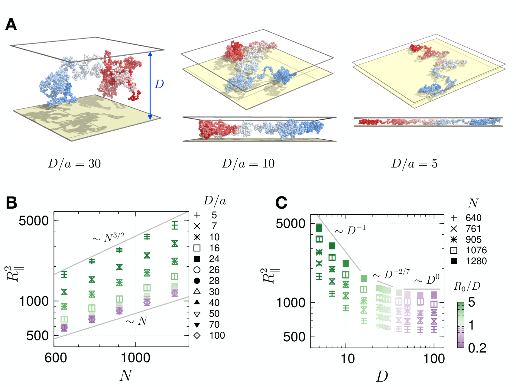
Next, the scaling of lateral size of polymer ($R_{\parallel}$) as the polymer of size $N>500$ is compressed from $R_{0}/D\gtrsim 1$ to $R_{0}/D\gg 1$ was examined (Fig.2). As shown in Fig.2B, the scaling relation of $R_{\parallel}^{2}\sim N$ is obeyed when the chain is effectively free from confinement ($R_{0}<D\simeq 100$). However, as the chain is compressed to the regime of strong confinement $D\ll R_{0}$, the scaling relationship for the self-avoiding chain in two dimensions, $R_{\parallel}^{2}\sim N^{3/2}$, is observed. The variation of scaling exponent $\nu$ from $\nu=1/2$ to $\nu=3/4$ with increasing compression is also found via the scaling relation between $R_{\parallel}$ and $D$ (Eq.3). Fig.2C shows the variation of $R_{\parallel}^{2}$ versus $D$ for five different values of $N$.

In fact, the exponent $\nu$ can be determined in terms of $R_{\parallel}$, $D$, $a$, and $N$.

$\displaystyle\nu=\frac{\log{(R_{\parallel}/D)}}{\log{\left[N(a/D)^{2}\right]}}$

(19)

Notice that $\Delta F\sim N(a/D)^{2}k_{B}T$ is the confinement free energy for an ideal chain in slit geometry, and that this free energy, $\Delta F\sim(N/g)k_{B}T$, corresponds to the energetic cost incurred in partitioning the original $\Theta$-chain into $N/g$ blobs. From Eq.5, a relationship between the confinement free energy and the lateral polymer size may be obtained, $\beta\Delta F=(R_{\parallel}/D)^{1/\nu}$. Using Eq.19, all of the data points from (Fig.2) collapse onto a single curve (Fig.3A). The slope of $R_{\parallel}/D$ versus $N(a/D)^{2}$ defines the scaling exponent $\nu$. For a given slit size $D$, the lateral dimension of the confined chain and its scaling exponent change with the extent of compression characterized by the quantity $N(a/D)^{2}$. The size exponent is $\nu=1/2$ for small $N(a/D)^{2}<1$ (for small compression $R_{0}/D<1$ or before the chain is split into multiple blobs); and plateaus $\nu=3/4$ for large $N(a/D)^{2}\gtrsim 10$ (for large compression $R_{0}/D\gtrsim 5$, or when more than 10 blobs of size $D$ are formed) (Fig.3A). This observation is made more explicit via the scaling exponent $\nu$ calculated by fitting five consecutive data points in Fig.3A. Fig.3B shows that there are two regimes where the value of $\nu$ plateaus over the range of compression.

As the extent of confinement is increased a $\Theta$-chain is found to swell. Its size scales with decreasing $D$ gradually changing from $R_{0}\sim aN^{1/2}$ to $R_{\parallel}^{\text{SAW}}\sim\tau aN^{3/4}(a/D)^{1/4}$. In comparison, the evidence for the conformal invariance prediction of $R_{\parallel}^{\Theta}\sim aN^{4/7}(a/D)^{1/7}$ is weak in Fig.3B. Two crossover points are identified in the scaling exponent $\nu$ as a function of $N(a/D)^{2}$: $N(a/D)^{2}\sim 1$ and $N(a/D)^{2}\sim 10$ (Fig.3B). The first crossover point $N(a/D)^{2}\sim 1$ arises from the condition when the confinement gap ($D$) is comparable to the size of the chain in free space, $D\sim R_{0}\simeq aN^{1/2}$. Further compression ($D<R_{0}$) perturbs the chain, which may be visualized as dividing it into multiple blobs. The plateau of $\nu=3/4$ is observed for $N(a/D)^{2}\gtrsim 10$. Although there is no clear evidence for the scaling exponent $\nu=4/7$, assuming that the second crossover point is obtained by equating $R_{\parallel}^{\Theta}$ and $R_{\parallel}^{\text{SAW}}$ yields $N(a/D)^{2}\sim\tau^{-28/5}(a/D)^{7/5}$. From this, it could be argued that the second crossover point is sensitive to the solvent quality given in terms of $\tau\left[=(T-T_{\Theta})/T_{\Theta}\right]$. Thus, in principle, the second crossover point may be at arbitrarily high confinement as $\tau$ approaches zero. However, the manifestation of SAW behavior at $N(a/D)^{2}\gtrsim 10$ (Fig.3B) implies either that the effect of higher order terms is no longer negligible or that the effect of second virial term becomes significant upon confinement.

In fact, the confinement alone effectively changes the pairwise monomer-monomer interaction which is controlled by the second virial coefficient ($B_{2}$) Glandt 1980; Yang et al. 2015; Krekelberg et al. 2019. Under slit confinement, $B_{2}$ changes as a function of $D$. For example, for a system comprised of Lennard Jones particles at the Boyle point (for a solution of small particles where the second virial coefficient vanishes), $B_{2}^{\text{LJ}}(D)$ can be derived by approximating the interparticle interaction as a square well potential of range of $\delta$ and depth $\epsilon$ (Fig.4A) as (see SI for details)

$\displaystyle B^{\text{LJ}}_{2}(D)=\begin{cases}\frac{\pi a^{3}(D/a)}{2}\left[\left\{\frac{5}{6}+\frac{1}{3}\frac{D}{a}-\frac{1}{6}\left(\frac{D}{a}\right)^{2}\right\}-(e^{\beta\epsilon}-1)\left\{2\frac{\delta}{a}+\left(\frac{\delta}{a}\right)^{2}\right\}\right]&(a<D\leq 2a),\\ \frac{\pi a^{3}(D/a)}{2(D/a-1)^{2}}\left[\left\{\frac{4}{3}\frac{D}{a}\psi(\epsilon,\delta)-\frac{24\psi(\epsilon,\delta)-13}{6}\right\}-\left(e^{\beta\epsilon}-1\right)\left\{6(\frac{\delta}{a})+5(\frac{\delta}{a})^{2}+\frac{4}{3}(\frac{\delta}{a})^{3}\right\}\right]&(D\geq 2a).\end{cases}$

(20)

In the above expression, $\psi(\epsilon,\delta)\left[\equiv 1+(1-e^{\beta\epsilon})\left(\left(1+\frac{\delta}{a}\right)^{3}-1\right)\right]$ is a factor that takes into account the effect of attraction in the square-well potential (see SI). In free space (i.e., $D\rightarrow\infty$) $B_{2}^{\text{LJ}}(D\rightarrow\infty)=\frac{2\pi}{3}a^{3}\psi(\epsilon,\delta)$. For the LJ system, the $\Theta$ condition (i.e., $B_{2}(\infty)=0$) is gained by setting $\psi(\epsilon,\delta)=0$. Remarkably, even for $\psi(\epsilon,\delta)=0$, $B^{\text{LJ}}_{2}(D)$ still increases from zero to positive values and is maximized to $\sim a^{3}$ at $D\approx 2a$ as $D$ is decreased (red curve in Fig.4C). In tight confinement ($D\ll R_{0}$) the second virial coefficient, originally tuned to zero, is no longer negligible.

In summary, in this study the effect of slit confinement on a single $\Theta$-chain in bulk was studied, focusing on the scaling behavior of the chain size with increasing compression. Instead of the transition of the scaling exponent from $\nu=1/2$ to $\nu=4/7$, which is expected for a $\Theta$-chain when the dimension is reduced from three to two, our numerical simulation displays the transition from $\nu=1/2$ to $\nu=3/4$ without a clear signature of $\nu=4/7$, which indicates that the solvent quality has effectively been changed from the $\Theta$ to good-solvent condition with increasing compression. By highlighting the effect of confining walls on the solvent quality, more specifically on the second virial coefficient, as well as the contribution from the higher order virial terms, this study shows that the tricritical $\Theta$-solvent condition is inherently unstable to reduction of dimensionality.

Finally, the variable solvent quality for polymer under confinement, highlighted in this study, can be related to one of the many factors that determine the stability of a biopolymer under nano-confinement or crowded condition Zhou and Dill 2001; Ziv et al. 2005; Cheung et al. 2005; Sorin and Pande 2006; Cheung and Thirumalai 2007; Lucent et al. 2007; Rasaiah et al. 2008; Mittal and Best 2008; Inomata et al. 2009; Lin et al. 2012; Malik et al. 2012; Ha and Jung 2015; Kim et al. 2015; Danielsson et al. 2015. Based on a consideration of the polymer conformational entropy, it is typically argued that confining a chain molecule alone entropically destabilizes the swollen conformations of chain and facilitates the collapse of the molecule. Interestingly, the results from this study based on a single $\Theta$-polymer under confinement suggest that the change in solvent quality from $B_{2}=0$ to $B_{2}>0$ engendered by confinement works in the direction that destabilizes the chain. Although solvent molecules are implicit, this study offers a possible explanation on why some experiments Malik et al. 2012; Inomata et al. 2009; Danielsson et al. 2015 and simulation studies, which explicitly considered solvent water molecules in conducting folding simulations of a protein molecule inside confinement Lucent et al. 2007; Sorin and Pande 2006, observe protein destabilization.

$\Theta$-polymer configurations in slit confinement with varying $D$ are generated using molecular simulation of a polymer described below.

References

- Daoud et al. (1975) Daoud, M.; Cotton, J. P.; Farnoux, B.; Jannink, G.; Sarma, G.; Benoit, H.; Duplessix, R.; Picot, C.; de Gennes, P. G. Solutions of Flexible Polymers. Neutron Experiments and Interpretation. Macromolecules 1975, 8, 804.
- Daoud and de Gennes (1977) Daoud, M.; de Gennes, P. G. Statistics of macromolecular solutions trapped in small pores. J. Phys. 1977, 38, 85–93.
- Tegenfeldt et al. (2004) Tegenfeldt, J. O.; Prinz, C.; Cao, H.; Chou, S.; Reisner, W. W.; Riehn, R.; Wang, Y. M.; Cox, E. C.; Sturm, J. C.; Silberzan, P.; Ausin, R. H. The dynamics of genomic-length DNA molecules in 100-nm channels. Proc. Natl. Acad. Sci. U. S. A. 2004, 101, 10979–10983.
- Hsu and Grassberger (2004) Hsu, H.-P.; Grassberger, P. Polymers confined between two parallel plane walls. J. Chem. Phys. 2004, 120, 2034–2041.
- Morrison and Thirumalai (2005) Morrison, G.; Thirumalai, D. The shape of a flexible polymer in a cylindrical pore. J. Chem. Phys. 2005, 122, 194907.
- Dimitrov et al. (2008) Dimitrov, D.; Milchev, A.; Binder, K.; Klushin, L. I.; Skvortsov, A. M. Universal properties of a single polymer chain in slit: Scaling versus molecular dynamics simulations. J. Chem. Phys. 2008, 128, 234902.
- Kang et al. (2015) Kang, H.; Yoon, Y.-G.; Thirumalai, D.; Hyeon, C. Confinement-induced glassy dynamics in a model for chromosome organization. Phys. Rev. Lett. 2015, 115, 198102.
- Ha and Jung (2015) Ha, B.-Y.; Jung, Y. Polymers under confinement: single polymers, how they interact, and as model chromosomes. Soft Matter 2015, 11, 2333–2352.
- Zhou and Dill (2001) Zhou, H.-X.; Dill, K. A. Stabilization of proteins in confined spaces. Biochemistry 2001, 40, 11289–11293.
- O’Brien et al. (2008) O’Brien, E.; Stan, G.; Thirumalai, D.; Brooks, B. Factors governing helix formation in peptides confined to carbon nanotubes. Nano letters 2008, 8, 3702–3708.
- Hsu and Grassberger (2005) Hsu, H.-P.; Grassberger, P. The coil–globule transition of confined polymers. J. Stat. Mech.: Theory and Experiment 2005, 2005, P01007.
- Cifra and Bleha (2000) Cifra, P.; Bleha, T. Concentration dependence of the global and anisotropic dimensions of confined macromolecules. Macromolecular theory and simulations 2000, 9, 555–563.
- Cifra and Teraoka (2003) Cifra, P.; Teraoka, I. Confined Polymer Chains in a Solvent: A Model with Polymer- Solvent Interactions. Macromolecules 2003, 36, 9638–9646.
- de Gennes (1975) de Gennes, P. G. Collapse of a polymer chain in poor solvents. J. Phys. Lett. 1975, 36, 55–57.
- Griffiths (1970) Griffiths, R. B. Thermodynamics near the two-fluid critical mixing point in He3-He4. Phys. Rev. Lett. 1970, 24, 715.
- Blume et al. (1971) Blume, M.; Emery, V.; Griffiths, R. B. Ising model for the transition and phase separation in He3-He4 mixtures. Phys. Rev. A 1971, 4, 1071.
- Halverson et al. (2014) Halverson, J. D.; Smrek, J.; Kremer, K.; Grosberg, A. Y. From a melt of rings to chromosome territories: the role of topological constraints in genome folding. Rep. Prog. Phys. 2014, 77, 022601.
- Liu and Hyeon (2016) Liu, L.; Hyeon, C. Contact statistics highlight distinct organizing principles of proteins and RNA. Biophys. J. 2016, 110, 2320–2327.
- Raphael and Pincus (1992) Raphael, E.; Pincus, P. A. Scaling theory of polymer solutsions trapped in small pores: the -solvent case. J. Phys. II France 1992, 2, 1341–1344.
- Vilanove and Rondelez (1980) Vilanove, R.; Rondelez, F. Scaling description of two-dimensional chain conformations in polymer monolayers. Phys. Rev. Lett. 1980, 45, 1502.
- Witte et al. (2010) Witte, K. N.; Kewalramani, S.; Kuzmenko, I.; Sun, W.; Fukuto, M.; Won, Y.-Y. Formation and collapse of single-monomer-thick monolayers of poly (n-butyl acrylate) at the air-water interface. Macromolecules 2010, 43, 2990–3003.
- Bunde and Gouyet (1985) Bunde, A.; Gouyet, J. F. On scaling relations in growth models for percolating clusters and diffusion fronts. J. Phys. A: Math. Gen. 1985, 18, L285–L287.
- Weinrib and Trugman (1985) Weinrib, A.; Trugman, S. A. A new kinetic walk and percolation perimeters. Phys. Rev. B. 1985, 31, 2993–2997.
- Grassberger (1986) Grassberger, P. On the hull of two-dimensional percolation clusters. J. Phys. A: Math. Gen. 1986, 19, 2675–2677.
- Coniglio et al. (1987) Coniglio, A.; Jan, N.; Majid, I.; Stanley, H. E. Conformation of a polymer chain at the point: Connection to the external perimeter of a percolation cluster. Phys. Rev. B 1987, 35, 3617.
- Duplantier and Saleur (1987) Duplantier, B.; Saleur, H. Exact Tricritical Exponents for Polymers at the Point in Two Dimensions. Phys. Rev. Lett. 1987, 59, 539–542.
- Duplantier and Saleur (1989) Duplantier, B.; Saleur, H. Stability of the polymer point in two dimensions. Phys. Rev. Lett. 1989, 62, 1368.
- Glandt (1980) Glandt, E. D. Density distribution of hard—spherical molecules inside small pores of various shapes. J. Colloid Interface Sci. 1980, 77, 512–524.
- Yang et al. (2015) Yang, J. H.; Schultz, A. J.; Errington, J. R.; Kofke, D. A. The rate of convergence of the virial series in confined systems. Mol. Phys. 2015, 113, 1179–1189.
- Krekelberg et al. (2019) Krekelberg, W. P.; Mahynski, N. A.; Shen, V. K. On the virial coefficients of confined fluids: Analytic expressions for the thermodynamic properties of hard particles with attractions in slit and cylindrical pores to second order. J. Chem. Phys. 2019, 150, 044704.
- Edwards and Singh (1979) Edwards, S. F.; Singh, P. Size of a polymer molecule in solution. Part 1.—Excluded volume problem. J. Chem. Soc. Faraday Trans. 2 1979, 75, 1001–1019.
- des Cloizeaux and Jannink (1990) des Cloizeaux, J.; Jannink, G. Polymers in solution: Their modelling and structure; Oxford University Press, 1990.
- Duplantier (1987) Duplantier, B. Geometry of polymer chains near the theta-point and dimensional regularization. J. Chem. Phys. 1987, 86, 4233–4244.
- Ziv et al. (2005) Ziv, G.; Haran, G.; Thirumalai, D. Ribosome exit tunnel can entropically stabilize -helices. Proc. Natl. Acad. Sci. U. S. A. 2005, 102, 18956.
- Cheung et al. (2005) Cheung, M. S.; Klimov, D.; Thirumalai, D. Molecular crowding enhances native state stability and refolding rates of globular proteins. Proc. Natl. Acad. Sci. U. S. A. 2005, 102, 4753–4758.
- Sorin and Pande (2006) Sorin, E. J.; Pande, V. S. Nanotube confinement denatures protein helices. J. Am. Chem. Soc. 2006, 128, 6316–6317.
- Cheung and Thirumalai (2007) Cheung, M.; Thirumalai, D. Effects of Crowding and Confinement on the Structures of the Transition State Ensemble in Proteins. J. Phys. Chem. B 2007, 111, 8250–8257.
- Lucent et al. (2007) Lucent, D.; Vishal, V.; Pande, V. S. Protein folding under confinement: a role for solvent. Proc. Natl. Acad. Sci. U. S. A. 2007, 104, 10430–10434.
- Rasaiah et al. (2008) Rasaiah, J. C.; Garde, S.; Hummer, G. Water in nonpolar confinement: from nanotubes to proteins and beyond. Annu. Rev. Phys. Chem. 2008, 59, 713–740.
- Mittal and Best (2008) Mittal, J.; Best, R. B. Thermodynamics and kinetics of protein folding under confinement. Proc. Natl. Acad. Sci. U. S. A. 2008, 105, 20233–20238.
- Inomata et al. (2009) Inomata, K.; Ohno, A.; Tochio, H.; Isogai, S.; Tenno, T.; Nakase, I.; Takeuchi, T.; Futaki, S.; Ito, Y.; Hiroaki, H.; Shirakawa, M. High-resolution multi-dimensional NMR spectroscopy of proteins in human cells. Nature 2009, 458, 106.
- Lin et al. (2012) Lin, P.-k.; Hsieh, C.-C.; Chen, Y.-L.; Chou, C.-F. Effects of topology and ionic strength on double-stranded DNA confined in nanoslits. Macromolecules 2012, 45, 2920–2927.
- Malik et al. (2012) Malik, A.; Kundu, J.; Mukherjee, S. K.; Chowdhury, P. K. Myoglobin unfolding in crowding and confinement. J. Phys. Chem. B 2012, 116, 12895–12904.
- Kim et al. (2015) Kim, J.; Jeon, C.; Jeong, H.; Jung, Y.; Ha, B.-Y. A polymer in a crowded and confined space: effects of crowder size and poly-dispersity. Soft Matter 2015, 11, 1877.
- Danielsson et al. (2015) Danielsson, J.; Mu, X.; Lang, L.; Wang, H.; Binolfi, A.; Theillet, F.-X.; Bekei, B.; Logan, D. T.; Selenko, P.; Wennerström, H.; Oliveberg, M. Thermodynamics of protein destabilization in live cells. Proc. Natl. Acad. Sci. U. S. A. 2015, 112, 12402–12407.
- Limbach et al. (2006) Limbach, H.-J.; Arnold, A.; Mann, B. A.; Holm, C. ESPResSo—an extensible simulation package for research on soft matter systems. Comp. Phys. Comm. 2006, 174, 704–727.
6 Supporting Information
6.1 The second virial coefficient of Lennard Jones particles in slit confinement
The second virial coefficient for hard-sphere (HS) system amounts to the volume of a spherical particle inaccessible to others. That is, the second virial coefficient for homogeneous hard sphere system with diameter , with for and for is given as . Geometrical confinement may be regarded as an external field applied to the particles, and it modifies the spatial distribution of a particle at with a factor , where is the potential energy that the particle experiences in the presence of the external field. The second virial coefficient of hard sphere system in slit confinement is given as Krekelberg et al. 2019