On the comparison of three numerical methods applied to building simulation: finite-differences, RC circuit approximation and a spectral method.
Abstract
Predictions of physical phenomena in buildings are carried out by using physical models formulated as a mathematical problem and solved by means of numerical methods, aiming at evaluating, for instance, the building thermal or hygrothermal performance by calculating distributions and fluxes of heat and moisture transfer. Therefore, the choice of the numerical method is crucial since it is a compromise among (i) the solution accuracy, (ii) the computational cost to obtain the solution and (iii) the complexity of the method implementation. An efficient numerical method enables to compute an accurate solution with a minimum computational run time (CPU). On that account, this article brings an investigation on the performance of three numerical methods. The first one is the standard and widely used finite-difference approach, while the second one is the so-called RC approach, which is a particular method brought to the building physics area by means of an analogy of electric circuits. The third numerical method is the spectral one, which has been recently proposed to solve nonlinear diffusive problems in building physics. The three methods are evaluated in terms of accuracy on the assessment of the dependent variable (temperature or vapor pressure) or of density of fluxes for three different cases: i) heat diffusion through a concrete slab, ii) moisture diffusion through an aerated concrete slab and iii) heat diffusion using measured temperatures as boundary conditions. Results highlight the spectral approach as the most accurate method. The RC based model with a few number of resistances does not provide accurate results for temperature and vapor pressure distributions neither to flux densities nor conduction loads.
a Univ. Grenoble Alpes, Univ. Savoie Mont Blanc, CNRS, LOCIE,
73000 Chambéry, France
b Univ. Grenoble Alpes, Univ. Savoie Mont Blanc, CNRS, LAMA, 73000 Chambéry, France
c Thermal Systems Laboratory, Mechanical Engineering Graduate Program,
Pontifical Catholic University of Paraná, Rua Imaculada Conceição, 1155, CEP : 80215-901,
Curitiba - Paraná, Brazil
∗Corresponding author. E-mail address: julien.berger@univ-smb.fr
keywords: Heat Transfer; Moisture Transfer; Numerical Methods; Finite Differences; Thermal Circuit Model; Spectral Method.
1 Introduction
As the building sector represents almost % of the world global energy consumption, current environmental issues lead to focus on energy efficiency of building envelopes Administration, 2015. Within this context, several tools have been developed since the ’s for the accurate assessment of building energy performance. Many of them have been reported in the frame of the International Energy Agency Annex published by Woloszyn and Rode in Woloszyn and Rode, 2008 and more recently in Mendes et al. Mendes et al., 2016.
Among all the physical phenomena involved in building energy efficiency, energy losses associated to heat and moisture transfer through the building envelope are of major importance. They represent an important part of building energy consumption and moisture may considerably impact on conduction loads and on the size of HVAC systems Mendes et al., 2003, besides promoting severe disorders when reaching high levels Berger et al., 2015. Thus, it is of primary importance to have numerical models enabling to accurately represent the physical phenomena for the evaluation of heat losses and gains through building envelopes.
The numerical models are elaborated from the main governing equations representing the heat and/or moisture transfer in building porous materials detailed for instance in Mendes et al., 2016. The use of analytical solutions is often limited due to the nonlinearity of the material properties and to the non-periodicity of the boundary conditions. Thus, most of models referenced in literature are based on numerical approaches.
Consequently, the main challenge arises in elaborating efficient numerical models to perform the simulation. The word efficiency can designate several features. One decisive aspect is the accuracy of the computed solution. It is of capital importance for the design of energy efficient buildings. To predict reliable energy consumption, one must be certain that the numerical errors of the model are negligible. When comparing the predictions to experimental observations, such as performed in Yang and Becerik-Gerber, 2015, researchers often assume that the numerical errors are always lower than the uncertainties present in the measurements, in the inputs parameters and in the mathematical model that described the physical phenomena. Another important feature is the computational run time of the numerical model to compute the solution. Even with the increase of computer power in the recent decades, it is still a crucial issue. The numerical model needs to save the computational efforts to ease the work of building designers and engineers. It is also relevant in the research context of sensitivity analysis or parameter estimation problem, where a large number of direct model computations is required.
Surprisingly, despite the widespread use of models in research and practice, the efficiency of the numerical models have received little attention in the literature. Models are implemented in software such as EnergyPlus Crawley et al., 2001, ESP-r Clarke, 2013, BSim Rode and Grau, 2003, etc. The governing equations are well detailed but the description of the numerical methods is generally brief and no discussion on their efficiency are provided. Moreover, the validity of the assumption that the numerical error can be negligible has never been verified. Thus, this article proposes to overcome this issue by presenting a detailed evaluation of the efficiency of the three numerical methods.
The first one, is the standard finite-differences based approach, which is probably the most-used method to compute the solution of the diffusion problem. Different variations of this approach have been reported in the literature such as the implicit Euler in Mendes and Philippi, 2005; Steeman et al., 2009, the explicit Euler in Tariku et al., 2010; Kalagasidis et al., 2007 or the Crank–Nicolson in Van Genuchten, 1982. The second method is the so-called RC approach. This method was first used during the second world war nad J. Lee et al., 1943 where analogous electric networks were built to solve the solution of transient heat-flow problems. Since there were no computer devices, it was an ingenuous way to rapidly simulate the solution of the problem. Interesting details can be found in Lawson and McGuire, 1953; Robertson and Gross, 1958 with an investigation of the error devices as a function of the number of (physical) thermal resistances. Although the appearance of digital computers started in the fifties and the rapid and progressive hardware evolution since the seventies, this RC method is still used in many algorithms to solve the partial differential equation of heat transfer as for instance in Fraisse et al., 2002; Roels et al., 2017; Naveros and Ghiaus, 2015. The third method is more advanced spectral method which was recently applied for the solution of diffusion problems through porous building elements Gasparin et al., 2018; Gasparin et al., 2017.
The manuscript is organized as follows. The physical problem of heat and moisture transfer in building porous materials is recalled in Section 2. The three numerical methods are described in Section 3. Then, three case studies are analysed. The first one, in Section 4, considers a linear heat transfer in a concrete wall. Then, in Section 5, a nonlinear case of moisture diffusion is investigated. In Section 6, the efficiencies of the numerical methods are evaluated considering real measured temperatures as boundary conditions. Some conclusion and final remarks are outlined in Section 8.
2 Physical problem and mathematical formulation
2.1 Physical phenomenon of heat transfer
The physical problem involves heat conduction in a wall of thickness composed of a single material in which the thermal conductivity is denoted as , the density as and the specific heat as . The problem can be formulated by the Fourier (or heat) equation, for and :
| (1) |
where is the temperature within the wall at the distance and time .
For the sake of simplicity11 1 Different approaches are reported in literature to represent the Neumann or Robin boundary conditions within the RC model framework. Thus, to limit the possible sources of error, the numerical investigation was performed considering Dirichlet boundary conditions. , Dirichlet boundary conditions are assumed at the extremity of the wall:
At the initial state, the temperature of the wall is assumed to be uniform:
One of the interesting outputs in the building physics framework is the heat flux density at , defined as:
| (2) |
Particularly, we denote as the heat flux density computed at :
The conduction loads represent the heat fluxes at the building envelope internal surface and, in terms of the energy density, it can be evaluated as:
| (3) |
which can be evaluated, for instance, over daily or monthly periods.
2.2 Physical phenomenon of moisture transfer
The moisture transfer occurs under isothermal conditions in a wall of thickness , with a single material of permeability and moisture capacity , both depending on the vapor pressure. The formulation of the problem, for and , yields to:
| (4) |
where is the vapor pressure within the wall.
The boundary conditions at the extremity of the wall are:
A uniform vapor pressure is assumed as initial condition:
The vapor flux density is similarly computed according to:
2.3 Dimensionless formulation
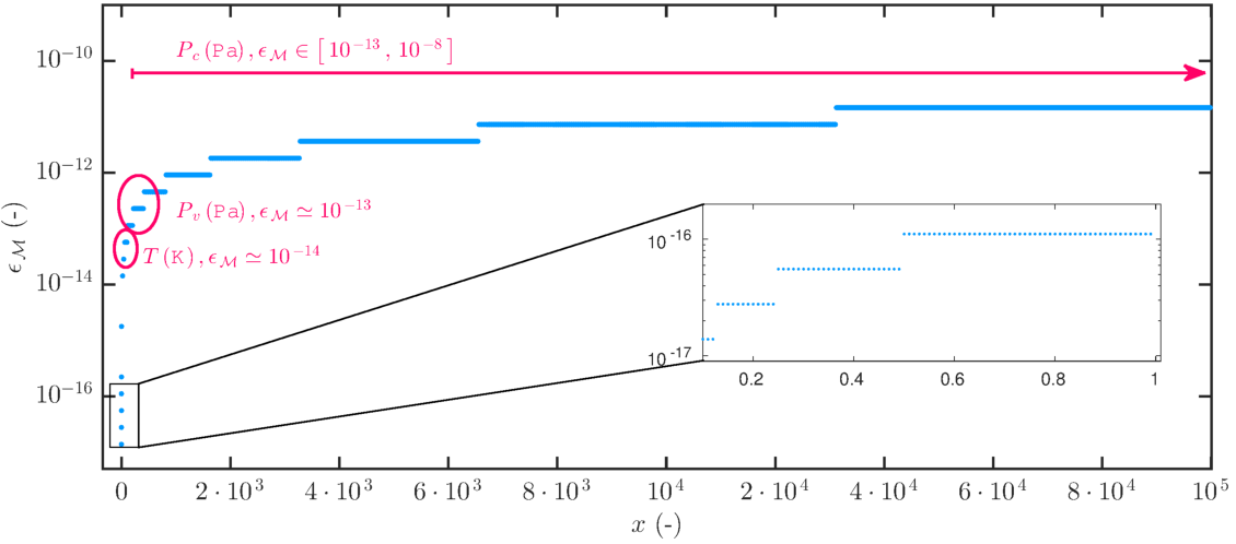
While performing a mathematical and numerical analysis of a given practical problem, it is of capital importance to obtain a unitless formulation of governing equations, due to a number of good reasons. First of all, it enables to determine important scaling parameters such as the Biot and Fourier numbers. Henceforth, solving one dimensionless problem is equivalent to solve a whole class of dimensional problems sharing the same scaling parameters. Then, dimensionless equations allow to estimate the relative magnitude of various terms, and thus, eventually to simplify the problem using asymptotic methods Nayfeh, 2000. Finally, the floating point arithmetics is designed such as the rounding errors are minimal if computer manipulates the numbers of the same magnitude Kahan and Palmer, 1979. Moreover, the floating point numbers have the highest density within the interval and their density decays exponentially when we move further away from zero. Figure 1 shows the accuracy of the floating points in Matlab™ environment. It is generated using the ) function in the Matlab environment. For a numerical model written using dimensionless equations, the accuracy of the floating points scales with . The potential commonly used in the physical model of heat and mass transfer is usually the temperature in , the vapor pressure or the capillary pressure both pressures in . According to Figure 1, if the numerical model is written using the temperature or the vapor pressure with their physical dimension, the accuracy of the floating points scales between and , respectively. The range of the capillary pressure is between and . Therefore, the accuracy of the floating point can loose up to orders compared to a dimensionless numerical model. So, it is always better to manipulate numerically the quantities of the order of to avoid severe round-off errors and to likely improve the conditioning of the problem in hands.
2.3.1 Heat transfer
In this way, according to Incropera et al., 2007, we define the following dimensionless quantities for the temperature:
The time and space domains are also modified through a unitless formulation:
where is a characteristic time. The Fourier dimensionless number is defined, characterizing the importance of the heat transfer through the material:
Therefore, the unitless system of the differential equation of heat transfer is formulated as:
| (5) |
together with the boundary conditions:
and the initial condition:
2.3.2 Mass transfer
In a very similar way, we define the following dimensionless quantities related to the vapor pressure field Luikov, 1966:
The unitless formulation of the time and space domains are:
The vapor pressure dependent moisture properties are transformed according to:
where and are reference property values. The Fourier dimensionless number is defined, characterizing here the importance of the moisture transfer through the material:
The Fourier number quantifies the first order of the diffusion transfer, while the dimensionless parameters and define the distortion or the nonlinearity of the phenomenon.
The unitless system of differential equation for moisture transfer is:
| (6) |
with the boundary conditions:
and the initial condition:
3 Numerical methods
In order to describe the numerical schemes, let’s first consider a uniform discretisation for simplicity of the interval :
For the RC model, the time layers are uniformly spaced as well , , . The values of the function in discrete nodes will be denoted by .
For the sake of simplicity, the standard finite-differences scheme and spectral approach will be described for the linear dimensionless heat diffusion equation (5). To our knowledge, the RC model is always described in the literature considering the physical dimension of the equation. In this way, the approach will be presented considering the heat diffusion equation (1).
3.1 The standard finite-differences method
The standard semi–discrete scheme based on central finite-differences can be written as:
| (7) |
whose starting value is directly obtained from the initial condition:
Many approaches can be used for the temporal discretisation of Eq. (7). Here the algorithm is implemented in Matlab™ environment using the function ode45 providing an efficient explicit Runge–Kutta scheme. In whole figures, this approach will be referenced as FDM.
3.2 The RC model
Both sides of the heat equation (1) is integrated over for the cell illustrated in Figure 2(a):
| (8) |
The average temperature of the cell is defined as
Thus, Eq. (8) becomes:
From the electric analogy of the heat conduction (Davies, 2004, Chap. 10), the heat flux is approximated by:
where is the thermal resistance defined as:
Finally, for each node , the temperature is computed using:
| (9) |
being the thermal capacity defined as:
The electric analogy of the heat conduction equation is illustrated in Figure 2(b). It can be noted that Eq. (9) corresponds to the central finite-differences discretisation of the second space derivative. The RC model states that the temperature can be computed using a user-defined number of resistances. Usually, such a model is denoted as with of the order of the unity . This hypothesis corresponds to compute the temperature using points of discretisation. It can also be seen as a low fidelity model to represent the physical phenomena of heat or moisture transfer in building porous material.
In this work, an Euler explicit approach is associated with the semi-discrete scheme (9), in agreement with Biddulph et al., 2014. In this case, it is important to note that the explicit scheme is only conditionally stable under the following Courant–Friedrichs–Lewy-type condition Courant et al., 1928:
| (10) |
The algorithm is implemented in the Matlab™ environment. Interested readers are invited to consult Davies, 2004; Fraisse et al., 2002 for more details on this approach and Deconinck and Roels, 2016; Reynders et al., 2014; Jimenez et al., 2009 for examples of applications in building physics.


3.3 The advanced spectral method
The spectral method has different approach, other than the central differences and thus, the RC ones. It assumes that the unknown from Eq. (5) can be approximately represented as a finite sum Mendes et al., 2016:
| (11) |
Here, is a set of basis functions that remains constant in time. In this study, the Chebyshev polynomials are used as the basis functions since they are optimal in approximation norm Gautschi, 2004. The functions are the corresponding time-dependent spectral coefficients. The parameter represents the number of degrees of freedom of the solution, also denoted as the order of the solution with . The main advantage of the spectral method is that , where is the number of degrees of freedom needed to solve problem (5) by means of conventional methods such as finite-differences, finite-volume or finite-element methods. For these reasons, the spectral method is also denoted as the spectral-Reduced Order Method (spectral-ROM) Gasparin et al., 2018; Gasparin et al., 2017.
The derivatives are written as follows:
| (12a) | ||||
| (12b) | ||||
| (12c) | ||||
where the dot denotes according to Newton notation. Using the properties of the Chebyshev polynomials, the space derivatives are re-expanded in the same Chebyshev basis function. The connection is explicitly given from the recurrence relation of the Chebyshev polynomial derivatives Peyret, 2002:
with,
Using the expression of the derivatives provided by Eqs. (12b) and (12c), the residual of the diffusion equation (5) is:
| (13) |
which is considered a misfit of the approximate solution. The purpose is to minimize the residual:
which is realised via the the Tau–Galerkin method, which requires Eq. (13) to be orthogonal to the Chebyshev basis functions . Here, the the scalar product is defined by :
Thus, it leads to the following relations among spectral coefficients:
Finally, after the projection and expansion of the residual, the original partial differential equation (5) is reduced to a system of ordinary differential equations plus two algebraic expressions enabling to compute the time dependent coefficients . For linear problems, the system of ordinary differential equations is explicitly built:
where , with constant coefficients, is a vector resulting from boundary conditions and is the vector of initial coefficients. Initial values of the coefficients are calculated by the Galerkin projection of the initial condition Canuto et al., 2006:
| (14) |
where , is the dimensionless initial condition. Interested readers may refer to Gasparin et al., 2018; Gasparin et al., 2017 for further details on the spectral method.
3.4 Extension of the methods for nonlinear problems
The extension of the three methods for nonlinear problem is now detailed. For the standard semi–scheme based on central finite-differences for Eq. (6), it is formulated as:
where
For the RC model, the extension for nonlinear problem in its physical dimension Eq. (4) is given by:
where is the vapor resistance and being the moisture capacity, both defined respectively as:
As described in Section 3.3, the unknown is approximated by the finite sum (11) with Chebyshev polynomials as basis functions. The derivatives are written as in the linear case, by Eqs. (12a), (12b) and (12c). Substituting them into Eq. (15), we get:
| (16) |
Then, the Tau–Galerkin method is used to minimize the residual of the equation. The integrals of the nonlinear coefficients and are computed using the Chebyshev–Gauß quadrature. At the end, it results in a system of Differential-Algebraic Equations (DAEs) with the following form:
where, is a diagonal and singular matrix containing the coefficients of the Chebyshev weighted orthogonal system, is a vector containing the boundary conditions and, is composed by the right member of Eq. (3.4) projected on the Chebyshev basis functions. The initial condition is given by Eq. (14) and the DAE system is solved by ode15s or ode23t from Matlab™.
3.5 Methods implementation and metrics of their efficiency
All the numerical algorithms for the classic and advanced schemes are written using dimensionless variables, while for the RC model, the physical dimensional variables are used. The numerical solutions are computed using an adaptive time step using Matlab™ function ode45 Shampine and Reichelt, 1997 with an absolute and relative tolerances set to . The efficiencies of the method are evaluated in terms of three criteria: (i) the global error of the numerical solution, (ii) the significant digits of the solution and (iii) the computational run time to compute the solution.
To evaluate the error, a reference solution is computed using a numerical pseudo–spectral approach obtained with the Matlab™ open source toolbox Chebfun Driscoll et al., 2014. Using the function pde23t, it permits to compute a numerical solution of a partial derivative equation using the Chebyshev functions. This useful package enables to compute reference solutions for one dimensional space-time problems. This tools is chosen since it can deal with more complex problems than analytical solution. Indeed, it can consider nonlinear coefficients or Robin-type time-dependent boundary conditions, which are more related to building physics application. The error between the solution, obtained by the numerical methods described above, and the reference one is computed as a function of by the following formula:
where is the number of temporal steps. The global uniform error is given by the maximum value of :
The significant correct digits of the solution are evaluated according to Soderling and Wang, 2006:
As the RC approach computes directly the fields in their physical dimension, a scaling transformation is performed to compute the errors. The last criteria is the computational (CPU) run time required by the numerical model to compute the solution. It is measured using the Matlab™ environment with a computer equipped with Intel i CPU and GB of RAM. We define the ratio:
where is the CPU time and is the final physical time of the simulation.
4 Numerical investigations: linear heat diffusion
Since the three methods have been presented, a first linear case of heat diffusion is considered to evaluate their efficiency, considering the following input values for a concrete slab:
The boundary conditions are defined as sinusoidal variations:
The temperature is computed using three RC model approaches with the thermal resistances . In addition, the problem is solved using the standard finite-differences method and spectral approach with modes. A spatial discretisation step is considered for both approaches. The temperature profiles at the last time of the simulation are shown in Figures 3 (a,b). It can be noted that the approaches with two or three resistances cannot compute an accurate temperature profile. A perfect agreement is observed between the reference and the solution computed using the RC, the standard finite-differences and the spectral approaches. The time evolution of the temperature in the middle of the wall is shown in Figures 4(a) and 4(b). Apparently, it seems that each approach enables to represent the temperature evolution. However, as shown in Figure 4(c), the difference with the reference solution can reach for the approach with two resistances. For the spectral approach, the difference is of the order .
One can argue that the differences, between the reference temperature and the one computed with the RC approach using two or three resistances, are acceptable. However, the discrepancy increases drastically for the heat flux density – which is directly dependent on the temperature derivative at the boundary –, going up to as highlighted in Figure 5(a). For the RC model with resistances, the heat flux density is computed with a very satisfying accuracy. As expected, similar results are observed for the standard finite-differences approach. The heat flux density is however more accurate when computed with the spectral approach. Figures 6(a) and 6(b) shows the error , computed using the dimensionless fields. It confirms that the temperature, computed with an RC model approach with only two or three resistances, lacks of accuracy to represent the physical phenomenon of heat diffusion. It should be noted that the error of the spectral method scales with with only modes. For the flux, the best accuracy reaches , which is obtained with the spectral approach. The error of the RC model with two or three resistances is completely unacceptable. It can be noted that the accuracy is more sensible to the heat flux density. This can also be understood by analyzing the propagation of the numerical errors. According to the definition in Eq. (2), the finite-difference approximation of the heat flux density is given by
If we consider that the temperature is computed with a numerical perturbation , with , the approximation of the heat flux is:
Since the perturbations are uncorrelated, and the approximation of the heat flux becomes
Since , the error on the heat flux density is higher than the one on the temperature. Considering the numerical values read in Figure 6(a), the numerical perturbation scales with for the standard finite-difference approach. With the spatial discretisation , the term is of the order . Thus, the error on the flux cannot be lower than this value. This value is in consistent with the results observed in Figure 6(b).
In terms of digits accuracy, the results are reported in Table 1. It is noticed the RC approach with resistances computes the field with more than twice digits accuracy than the RC one. The spectral method presents the highest accuracy. For the computational time, as expected, the numerical models with and resistances are the fastest approach. Indeed they require a very few computations at each time step ( and , respectively). However, the speed of computation decreases with the accuracy of the solution. The computational effort of the standard finite-difference approach scales with the RC one for resistances. A good compromise between speed of computation and accuracy is the Spectral approach.


These results highlight that the RC model with a small number of resistance cannot provide an accurate solution. A natural question rises: how many resistances are required to accurately compute the temperature within the wall? The answer to this question strongly depends on the numerical values of the application. For this case study, the error with the reference solution has been computed as a function of the resistance number , as shown in Figure 7. If the field of interest is the temperature, it can be noted that a number of resistances is sufficient. The error remains stable at corresponding to the tolerance set in the ode45 solver of the Matlab™ environment. Although, if one is interested in the heat flux density, the minimum number is to reach an error lower than .

| Numerical Model | for | for | ||
|---|---|---|---|---|
| RC | ||||
| RC | ||||
| RC | ||||
| FDM | ||||
| Spectral |
5 Numerical investigations: nonlinear moisture diffusion
The previous section considered a linear model of diffusion. It is important to evaluate the performance of the methods for nonlinear problems since the accuracy of the solution can be deteriorated. For this, a nonlinear moisture diffusion problem is considered. The length of the wall is set to and the simulation horizon to . The material properties are inspired from Bednar and Hagentoft, 2005 with a constant moisture capacity and a vapor pressure dependent moisture permeability:
Sinusoidal variations are imposed as boundary conditions:
where is the saturation pressure at . These conditions correspond to variations around the relative humidity to the dry and almost-saturated states.
The solution to problem (4) is computed using the RC approaches for , the standard finite-differences one and the spectral one with modes. For the last two methods, the spatial discretisation is . The profile of vapor pressure at is shown in Figure 8 (a,b). The time evolution of the vapor pressure in the middle of the layer is given in Figures 9(a) and 9(b). The standard finite-differences and spectral approaches represent accurately the field evolution. On the contrary, an important discrepancy is noted for the approach using two or three resistances (at the order of ). The differences become more important when looking at the moisture flux density, illustrated in Figures 10(a) and 10(b). The flux is underestimated by the RC approach based on a few resistances. If we look at Figures 11(a) and 11(b), the absolute differences of the flux reach for the RC approach. However, as shown in Figure 11(c) and 11(d), for these approaches the relative difference on the flux scales with for a field of the same order of magnitude. The global error for each approach is given in Figure 12. The most accurate approach is the spectral one, with an error at the order . Due to the nonlinearity of the problem, the error of the RC approach, with two or three resistances, have increased when compared to the previous case. As mentioned in the previous case, the error is more important for the RC and RC approaches since the space derivative of the field is computed with a low accuracy as illustrated in Figure 13.
The accuracy digits of each method are reported in Table 2. The digit accuracy of the RC approach with a few number of resistance is much lower compared to the previous case. This lack of accuracy may also be due to the computation of the solution in its physical dimension. Where the temperature scales with in the previous case, here the vapor pressure scales with . It may introduce additional computational rounding errors. For the spectral approach, it remains stable with four digits of accuracy in the computed vapor pressure. In terms of computational time, the RC and RC have low computational ratio. However, these methods lack of accuracy to compute the fields, particularly the moisture flux density. The Spectral method has the best efficiency providing an accurate solution at a reasonable computational cost.
A parametric study on the number of resistances have been carried out and the error is shown in Figure 14. Compared to the previous case of linear diffusion, more resistances are required to reach a satisfying accuracy. A minimal number of and resistances are necessary to represent accurately the vapor pressure or moisture flux evolution, respectively.


| Numerical Model | for | for | ||
|---|---|---|---|---|
| RC | ||||
| RC | ||||
| RC | ||||
| FDM | ||||
| Spectral |
6 Evaluating the methods efficiencies for a real case study
6.1 Description
The purpose is to evaluate now the efficiencies of the numerical methods considering a more realistic case study of heat transfer. The fields were assessed on a building built in Bayonne, France, at the end of the Century. With three basements, a west-oriented wall, located at the first floor in the living room, was monitored. Two calibrated monitoring sensors HOBO TMC––HA were placed at the surface of the wall, as shown in Figure 15(a). A thermal conductive paste was added on the sensor to reduce the contact resistance. An insulated protection has also been placed to avoid incident radiation on the sensors. The location of the sensors was chosen on a part of the wall where heat transfer can be supposed as uni-dimensional between inside and outside ambient. The data measurements were stored with a period of during one year. Interested readers are invited to consult Cantin et al., 2010; Berger et al., 2016 for complementary information.
In Berger et al., 2016, complementary measures were used to estimate the thermal conductivity of the wall. Here, the purpose is to use the surface one year measurements to provide the boundary conditions. As shown in Figure 15(b), there are distinguished daily variations with a raising between and , corresponding to the summer season.
The wall is considered as homogeneous using the following thermal properties: for the thermal conductivity, for the volumetric heat capacity. Considering the length of the wall and a reference time of , the Fourier dimensionless number equals .
For this real and occupied building the initial condition is not known. In addition, the installation of the sensors may cause perturbations on the thermal behavior of the wall. Thus, the first seven days of measurements are discarded and a linear reconstruction between the measured temperatures at given locations was considered as the initial condition at .


6.2 Results and discussion
The temperature is computed within the wall using the RC with resistances, the standard finite-differences and the spectral approaches. For the last two methods, the spatial discretisation is . For the last two methods, the spatial discretisation is . No reference solution is computed for this case. Thus, as the spectral method was shown as the most precise method in the previous cases, it was used as a reference to compute the absolute temperature difference for the standard finite-differences and RC approaches, illustrated in Figures 16(a) and 16(c). The standard finite-differences approach has less discrepancies with the spectral solution than the RC one. The maximum difference for the RC reaches . As shown in Figures 16(b) and 16(d), there is good agreement between the RC, standard finite-differences and spectral solutions. As expected, the RC approach with a sufficient high number of resistances enables to accurately represent the physical phenomenon. The heat flux at the right boundary is shown in Figures 17(b) and 17(d). More important discrepancies are noted between the RC approaches with two or three resistances than for the other solutions. In addition, the absolute difference with the spectral solution reaches for the RC approach. For the standard finite-differences solution, the difference remains lower than .
In terms of computational cost, the ratio of CPU time is for the RC, for the RC, for the RC, by using the finite-difference approach and by the spectral model. The latter presents the best efficiency to compute the solution of the problem.
It can be noted that the daily and monthly averaged temperatures are well represented by all methods, as shown in Figures 18(a) and 18(b). There is a perfect agreement among all solutions. The conduction loads are presented in Figures 19(a) and 19(b). For the analysis on the monthly period, the conduction loads are negative for a ten-month period corresponding to winter time. During the summer, the loads are positive, indicating an inward heat flux density. Globally, all the numerical methods enable to estimate the conduction loads with the same order of accuracy. No important discrepancies are noted. This is due to the definition of the heat loads from Eq. (3). The integration is performed for a monthly period. As noticed in Figure 17(b), the RC approximates well the mean heat flux, compared to the RC approach. Therefore, when integrating during a monthly period, the error on the conduction loads is smoothed. On the contrary, when looking at the daily loads of a winter period in Figure 19(b), the discrepancies among the three methods are higher. Particularly, the RC and RC solutions lack of accuracy.
These results lead to the conclusion that the choice of the methods depends on the characteristic timescale of the selected output. If the issue is to accurately analyze the physical phenomenon at a short time scale, then the methods (i) standard finite-differences, (ii) spectral and (iii) RC with a sufficient enough number of resistances, provide a sufficient accuracy. If the output evolves on a relatively large time scale, the RC approach with a few number of resistances may provide a satisfactory approximation of the physical phenomenon.


7 Synopsis of the discussions
It is of major importance to have efficient numerical methods to investigate physical phenomena associated to heat or moisture diffusion through building envelopes. Building simulation programs detail the governing equations but the efficiency of the numerical methods is rarely discussed. This article proposed to investigate the efficiency of three methods by evaluating their accuracy and calculation speed. The first one is the standard one based on central finite-differences and on the Runge–Kutta explicit approach. The second method is the so-called RC model. This approach was initially used to build analogous electric devices to simulate the heat conduction in the ’s–’s. It was then implemented in the computer algorithm and is still used for educational, research and regulation purposes in building physics. The last method is the spectral reduced order method. It has been recently proposed for building simulation purposes in Gasparin et al., 2018; Gasparin et al., 2017.
Three case studies have been presented in Section 4, a case of linear heat diffusion was considered. The solutions were computed using the three approaches and compared to a reference solution. The results highlighted that accuracy is satisfactory for the standard finite-differences, the RC and the spectral approaches. Among the three methods, the spectral is the most accurate with the higher number of digits accuracy. It actually gives a good compromise between accuracy and calculation speed. When using a low number of thermal resistances, the accuracy of the RC approach decreases with an absolute difference of the order of with the reference solution. However, the accuracy is lower when looking at the flux density. Indeed, the RC and RC approximate the flux with an absolute difference of the order . A parametric study was performed to evaluate the minimal number of thermal resistances to reach a satisfactory precision. For this case study, the minimal number is around and resistances for the temperature and the heat flux, respectively.
A similar numerical investigation was then accomplished for a case of nonlinear moisture diffusion, in Section 5. The results are very similar and highlight the spectral method is again the most accurate approach with a reasonable computational run time. The speed of computation of the RC and RC models is very low. However, the speed of computation decreases with the accuracy of the solution. It was noted that the number of significant digits of the RC and RC solutions was much lower than for the previous linear case study due mainly to two reasons. First, this case considered a non-linear problem inducing more errors for coarse approaches. Then, the RC approach computes the solution directly in its physical dimension where the others consider a dimensionless formulation of the problem. The vapor pressure scales with where the temperature with . Therefore, additional computational rounding errors may be introduced in the second case study since the errors of the floating point arithmetic of the computers are minimal for quantities of the magnitude . The minimal number of resistances to reach a sufficient accuracy with the RC approach was and for the temperature and the heat flux outputs of interest, respectively.
The third case study was more realistic case with real measured temperature as boundary condition for the study of heat transfer in a Century building wall. The simulation was performed for . No reference solution was available for this case. The standard finite-differences, RC and spectral methods had similar tendencies to represent the temperature evolution in the wall. The RC approach showed a maximum absolute difference of with the spectral solution. For the heat flux, the absolute differences were of the order of between both approaches. Within the context of energy efficiency, a relevant output is the time-integrated conduction loads. The latter were calculated for both monthly and daily periods. All the methods have very similar tendencies to estimate the monthly conduction loads. Nevertheless, the RC and RC approaches reveal significant discrepancies with the others when looking at the daily loads. It is due to the integration periods and the fact that the RC approaches with a few temperature approximates well the time mean of the heat flux.
8 Conclusion
With the issue of elaborating reliable models to predict some physical phenomena involved in building energy efficiency, the selection of the numerical methods has to be done considering the characteristic time scale of the aimed output, among other criteria. For the analysis of physical phenomena in a short time scale it is better to use the methods (i) standard finite differences, (ii) spectral or (iii) RC with a sufficient number of resistances. The RC model with a few number of resistances decreases the order of the model. With three resistances for instance, the number of degrees of freedom is only two, reducing consequently the computational effort to solve the problem. However, the fidelity of the model to represent the physical phenomena of heat or moisture transfer is strongly impacted and lacks of accuracy. These results are corroborated with the ones presented in Kircher and Zhang, 2015. With the issue of reducing the computational effort, the spectral method is the most efficient among the three approaches. Indeed, a model with less than degrees of freedom enables to compute the most accurate solution among the other approaches. Another important point concerns the computation of the surface density of fluxes at the boundaries. The numerical approximation to compute the fluxes introduces errors so that the accuracy is generally decreased compared to the one of the governing fields (temperature or vapor pressure). Since the fluxes are of capital importance on the design of energy efficient buildings, the accuracy of the numerical method to compute them should always been carefully verified.
All these results were obtained on rather a simple case study. The physical phenomena are more complex, involving coupled heat and mass transfer and Robin–type boundary conditions with radiation heat transfer and wind-driven rain. Therefore, before analyzing the physical phenomena in building physics, it is of capital importance to compare the accuracy of the numerical model, including the mathematical formulation of the physical problem together with the numerical methods and the discretisation mesh, with a reference solution. This procedure has to be carried out keeping in mind the output of interest.
Nomenclature
| Latin letters | ||
|---|---|---|
| conduction loads | ||
| specific heat capacity | ||
| vapor flux density | ||
| thermal conductivity | ||
| capillary pressure | ||
| vapor pressure | ||
| heat flux density | ||
| time coordinate | ||
| temperature | ||
| space coordinate | ||
| Greek letters | ||
|---|---|---|
| moisture permeability | ||
| density | ||
| moisture capacity | ||
Acknowledgments
The authors acknowledge the Brazilian Agencies CAPES of the Ministry of Education, the CNPQ of the Ministry of Science, Technology and Innovation, for the financial support for the project CAPES-COFECUB Ref. 774/2013 as well as the support of CNRS/INSIS (Cellule énergie) under the program “Projets Exploratoires — 2017”. The authors also acknowledge the Junior Chair Research program “Building performance assessment, evaluation and enhancement” from the University of Savoie Mont Blanc in collaboration with The French Atomic and Alternative Energy Center (CEA) and Scientific and Technical Center for Buildings (CSTB).
References
- Administration, (2015) Administration, U. E. I. (2015). Annual Energy Outlook 2015, with projections to 2040. EIA, Washington.
- Bednar and Hagentoft, (2005) Bednar, T. and Hagentoft, C. (2005). Analytical solution for moisture buffering effect validation exercises for simulation tools. Reykjavik, Iceland. Chalmers Publication Library (CPL), 7th Nordic Symposium on Building Physics,.
- Berger et al., (2015) Berger, J., Guernouti, S., Woloszyn, M., and Buhe, C. (2015). Factors governing the development of moisture disorders for integration into building performance simulation. Journal of Building Engineering, 3:1–15.
- Berger et al., (2016) Berger, J., Orlande, H., Mendes, N., and Guernouti, S. (2016). Bayesian inference for estimating thermal properties of a historic building wall. Building and Environment, 106(Supplement C):327 – 339.
- Biddulph et al., (2014) Biddulph, P., Gori, V., Elwell, C., Scott, C., Rye, C., Lowe, R., and Oreszczyn, T. (2014). Inferring the thermal resistance and effective thermal mass of a wall using frequent temperature and heat flux measurements. Energy and Buildings, 78(Supplement C):10 – 16.
- Cantin et al., (2010) Cantin, R., Burgholzer, J., Guarracino, G., Moujalled, B., Tamelikecht, S., and Royet, B. (2010). Field assessment of thermal behaviour of historical dwellings in France. Building and Environment, 45(2):473 – 484.
- Canuto et al., (2006) Canuto, C., Hussaini, M. Y., Quarteroni, A., and Zang, T. A. (2006). Spectral Methods - Fundamentals in Single Domains. Scientific Computation. Springer Berlin Heidelberg, Berlin, Heidelberg.
- Clarke, (2013) Clarke, J. (2013). Moisture flow modelling within the esp-r integrated building performance simulation system. Journal of Building Performance Simulation, 6(5):385–399.
- Courant et al., (1928) Courant, R., Friedrichs, K., and Lewy, H. (1928). Über die partiellen Differenzengleichungen der mathematischen Physik. Mathematische Annalen, 100(1):32–74.
- Crawley et al., (2001) Crawley, B. D., Lawrie, L. K., Winkelmann, F. C., Buhl, W., Huang, Y., Pedersen, C. O., Strand, R. K., Liesen, R. J., Fisher, D. E., Witte, M. J., and Glazer, J. (2001). Energyplus: creating a new-generation building energy simulation program. Energy and Buildings, 33(4):319 – 331.
- Davies, (2004) Davies, M. G. (2004). Building Heat Transfer. John Wiley & Sons, England.
- Deconinck and Roels, (2016) Deconinck, A. and Roels, S. (2016). Comparison of characterisation methods determining the thermal resistance of building components from onsite measurements. Energy and Buildings, 130(Supplement C):309 – 320.
- Driscoll et al., (2014) Driscoll, T. A., Hale, N., and Trefethen, L. N. (Oxford 2014). Chebfun guide. Pafnuty Publications.
- Fraisse et al., (2002) Fraisse, G., Viardot, C., Lafabrie, O., and Achard, G. (2002). Development of a simplified and accurate building model based on electrical analogy. Energy and Buildings, 34(10):1017 – 1031.
- Gasparin et al., (2017) Gasparin, S., Berger, J., Dutykh, D., and Mendes, N. (2017). Advanced reduced-order models for moisture diffusion in porous media. Transport in Porous Media, 0(0):1–30.
- Gasparin et al., (2018) Gasparin, S., Berger, J., Dutykh, D., and Mendes, N. (2018). Solving nonlinear diffusive problems in buildings by means of spectral methods. Journal of Building Performance Simulation, 0(0):1–20.
- Gautschi, (2004) Gautschi, W. (2004). Orthogonal Polynomials: Computation and Approximation. Oxford University Press, Oxford.
- Incropera et al., (2007) Incropera, F., Dewitt, D., Bergman, T., and Lavine, A. (2007). Fundamentals of Heat and Mass Transfer, 6th edition. John Wiley & Sons, England.
- Jimenez et al., (2009) Jimenez, M., Porcar, B., and Heras, M. (2009). Application of different dynamic analysis approaches to the estimation of the building component U value. Building and Environment, 44(2):361 – 367.
- Kahan and Palmer, (1979) Kahan, W. and Palmer, J. (1979). On a proposed floating-point standard. ACM SIGNUM Newsletter, 14:13–21.
- Kalagasidis et al., (2007) Kalagasidis, A., Weitzmann, P., Nielsen, T., Hagentoft, R. P. C., and Rode, C. (2007). The international building physics toolbox in simulink. Energy and Buildings, 39(6):665–674.
- Kircher and Zhang, (2015) Kircher, K. J. and Zhang, K. M. (2015). On the lumped capacitance approximation accuracy in RC network building models. Energy and Buildings, 108(Supplement C):454 – 462.
- Lawson and McGuire, (1953) Lawson, D. I. and McGuire, J. H. (1953). The solution of transient heat-flow problems by analogous electrical networks. Proceedings of the Institution of Mechanical Engineers, 167(1):275–290.
- Luikov, (1966) Luikov, A. (1966). Heat and Mass Transfer in Capillary-Porous Bodies. Pergamon, Oxford.
- Mendes et al., (2016) Mendes, N., Chhay, M., Berger, J., and Dutykh, D. (2016). Numerical methods for diffusion phenomena in building physics. PUC Press, Curitiba.
- Mendes and Philippi, (2005) Mendes, N. and Philippi, P. C. (2005). A method for predicting heat and moisture transfer through multilayered walls based on temperature and moisture content gradients. International Journal of Heat and Mass Transfer, 48(1):37–51.
- Mendes et al., (2003) Mendes, N., Winkelmann, F., Lamberts, R., and Philippi, P. (2003). Moisture effects on conduction loads. Energy and Buildings, 35(7):631 – 644.
- nad J. Lee et al., (1943) nad J. Lee, S. K., Olive, T., Batters, H., Callaham, J., Farquhar, N., and Pope, L. (1943). Complex heat transfer solved by electrical analogy. Chemical and Metallurgical Engineering, 50(12):111–113.
- Naveros and Ghiaus, (2015) Naveros, I. and Ghiaus, C. (2015). Order selection of thermal models by frequency analysis of measurements for building energy efficiency estimation. Applied Energy, 139(Supplement C):230 – 244.
- Nayfeh, (2000) Nayfeh, A. (2000). Perturbation Methods. Wiley VCH.
- Peyret, (2002) Peyret, R. (2002). Spectral methods for incompressible viscous flow. Springer, New York.
- Reynders et al., (2014) Reynders, G., Diriken, J., and Saelens, D. (2014). Quality of grey-box models and identified parameters as function of the accuracy of input and observation signals. Energy and Buildings, 82(Supplement C):263 – 274.
- Robertson and Gross, (1958) Robertson, A. . F. and Gross, D. (1958). An electrical-analog method for transient heat-flow analysis. Journal of Research of the National Bureau of Standards, 61(2):1–12.
- Rode and Grau, (2003) Rode, C. and Grau, K. (2003). Whole Building Hygrothermal Simulation Model. ASHRAE Transactions, 109(1):572–582.
- Roels et al., (2017) Roels, S., Bacher, P., Bauwens, G., Castaño, S., Jiménez, and Madsen, H. (2017). On site characterisation of the overall heat loss coefficient: comparison of different assessment methods by a blind validation exercise on a round robin test box. Energy and Buildings, 153:179–189.
- Shampine and Reichelt, (1997) Shampine, L. and Reichelt, M. (1997). The MATLAB ODE suite. SIAM J. Sci. Comput., 18(-):1–22.
- Soderling and Wang, (2006) Soderling, G. and Wang, L. (2006). Evaluating numerical ODE/DAE methods, algorithms and software. Journal of Computational and Applied Mathematics, 185:244–260.
- Steeman et al., (2009) Steeman, H.-J., Van Belleghem, M., Janssens, A., and De Paepe, M. (2009). Coupled simulation of heat and moisture transport in air and porous materials for the assessment of moisture related damage. Building and Environment, 44(10):2176–2184.
- Tariku et al., (2010) Tariku, F., Kumaran, K., and Fazio, P. (2010). Transient model for coupled heat, air and moisture transfer through multilayered porous media. International Journal of Heat and Mass Transfer, 53(15–16):3035–3044.
- Van Genuchten, (1982) Van Genuchten, M. (1982). A comparison of numerical solutions of the one-dimensional unsaturated-saturated flow and transport equations. Advances in Water Resources, 5(1):665–674.
- Woloszyn and Rode, (2008) Woloszyn, M. and Rode, C. (2008). Tools for performance simulation of heat, air and moisture conditions of whole buildings. Building Simulation, 1(1):5–24.
- Yang and Becerik-Gerber, (2015) Yang, Z. and Becerik-Gerber, B. (2015). A model calibration framework for simultaneous multi-level building energy simulation. Applied Energy, 149:415 – 431.