Monotonic Gaussian Process Flows
Ivan Ustyuzhaninov∗ Ieva Kazlauskaite∗ Carl Henrik Ek Neill D. F. Campbell
University of Tübingen University of Bath, Electronic Arts University of Bristol University of Bath, Royal Society
Abstract
We propose a new framework for imposing monotonicity constraints in a Bayesian nonparametric setting based on numerical solutions of stochastic differential equations. We derive a nonparametric model of monotonic functions that allows for interpretable priors and principled quantification of hierarchical uncertainty. We demonstrate the efficacy of the proposed model by providing competitive results to other probabilistic monotonic models on a number of benchmark functions. In addition, we consider the utility of a monotonic random process as a part of a hierarchical probabilistic model; we examine the task of temporal alignment of time-series data where it is beneficial to use a monotonic random process in order to preserve the uncertainty in the temporal warpings. †† * Equal contribution
1 INTRODUCTION
Monotonic regression is a task of inferring the relationship between a dependent variable and an independent variable when it is known that the relationship is monotonic. Monotonic functions (and monotonic random processes) have previously been studied in areas as diverse as physical sciences for estimating the temperature of a cannon barrel over time [Lavine and Mockus, 1995], marine biology for surveying of fauna on the seabed of the Great Barrier Reef [Hall and Huang, 2001], geology for chronology of sediment samples [Haslett and Parnell, 2008], public health for relating obesity and body fat [Dette and Scheder, 2006], sociology for relating education, work experience and salary [Dette and Scheder, 2006], design of computer networking systems [Golchi et al., 2015], economics for estimating personal income [Canini et al., 2016], insurance for predicting mortality rates [Durot and Lopuhaä, 2018], biology of establishing the diagnostic value of bio-markers for Alzheimer’s disease and for trajectory estimation in brain imaging [Lorenzi et al., 2019, Nader et al., 2019], meteorology for estimation of wind-induced under-catch of winter precipitation [Kim et al., 2018] and others.
Monotonicity also appears in the more general context of hierarchical models where we want to transform a (simple and typically stationary) input distribution to a (complicated and non-stationary) data distribution. More specifically, monotonicity constraints have been used in hierarchical models with warped inputs, for example, in Bayesian optimisation of non-stationary functions [Snoek et al., 2014] and in mixed effects models for temporal warps of time-series data [Kaiser et al., 2018, Kazlauskaite et al., 2019, Raket et al., 2016].
Extensive study by the statistics [Ramsay, 1988, Sill and Abu-Mostafa, 1997] and machine learning communities [Riihimäki and Vehtari, 2010, Andersen et al., 2018] has resulted in a variety of frameworks. While many traditional approaches use constrained parametric splines, they are not sufficiently expressive and, typically, do not include prior beliefs about the characteristics of the underlying function (such as smoothness). Consequently, many contemporary methods consider monotonicity in the context of continuous random processes, mostly based on Gaussian processes (GPs) [Rasmussen and Williams, 2005]. As a nonparametric Bayesian model, a GP is an attractive foundation on which to build flexible and theoretically sound models with well-calibrated estimates of uncertainty and automatic complexity control. However, imposing monotonicity constraints on a GP has proven to be problematic [Lin and Dunson, 2014, Riihimäki and Vehtari, 2010] as it requires both formulating a prior that is monotonic as well as constraining the (predictive) posterior to be monotonic. This is particularly challenging as monotonicity is a global property, implying that the function values are correlated for all inputs, irrespective of the lengthscale of the covariance [Andersen et al., 2018].
In this work we propose a novel nonparametric Bayesian model of monotonic functions that is based on the recent work on differential equations (DEs). At the heart of such models is the idea of approximating the derivatives of a function rather than studying the function directly. DE models have gained a lot of popularity recently and they have been successfully applied in conjunction with both neural networks [Chen et al., 2018] and GPs [Heinonen et al., 2018, Yildiz et al., 2018a, Yildiz et al., 2018b]. We consider a recently proposed framework, called differential GP flows [Hegde et al., 2019], that performs classification and regression by learning a stochastic differential equation (SDE) transformation of the input space. It admits an expressive yet computationally convenient parametrisation using GPs.
Utilising the uniqueness theorem for the solutions of SDEs [Øksendal, 1992], we formulate a novel stochastic random process that is guaranteed to be monotonic. We show that, unlike some of the previous work on monotonic random processes, the proposed approach is guaranteed to lead to monotonic samples from the model (defined as a flow field), and it performs competitively on a set of regression benchmarks.
Furthermore, we study an illustrative example of a hierarchical, two-layer model where the first layer corresponds to a smooth monotonic warping of time and the second layer corresponds to a sequence of time-series observations. The overall goal in such a problem is to learn the warpings of the inputs such that the unwarped versions of the sequences are temporally aligned. While such models typically rely on parametric transformations for the temporal warpings [Kazlauskaite et al., 2019], we show how the estimation of uncertainty leads to a model that is more informative and more interpretable than the previous approach. To achieve this, we further make use of the recent advances in variational inference for deep GPs [Ustyuzhaninov et al., 2019] to capture the compositional uncertainty present in the hierarchical model.
2 RELATED WORK
Splines
Many classical approaches to monotonic regression rely on spline smoothing: given a basis of monotone spline functions, the underlying function is approximated using a non-negative linear combination of these basis functions and the monotonicity constraints are satisfied in the entire domain [Wahba, 1978] by construction. For example, Ramsey [Ramsay, 1998] considers a family of functions defined by the differential equation which contains the strictly monotone twice differentiable functions, and approximates using a basis of M-splines and I-splines. Shively et al. [Shively et al., 2009] consider a finite approximation using quadratic splines and a set of constraints on the coefficients that ensure isotonicity at the interpolation knots. The use of piecewise linear splines was explored by Haslett and Parnell [Haslett and Parnell, 2008] who use additive i.i.d. gamma increments and a Poisson process to locate the interpolation knots; this leads to a process with a random number of piecewise linear segments of random length, both of which are marginalised analytically. Further examples of spline based approaches rely on cubic splines [Wolberg and Alfy, 2002], mixtures of cumulative distribution functions [Bornkamp and Ickstadt, 2009] and an approximation of the unknown regression function using Bernstein polynomials [Curtis and Ghosh, 2011].
Gaussian process
A GP is a stochastic process which is fully specified by its mean function, , and its covariance function, , such that any finite set of random variables have a joint Gaussian distribution [Rasmussen and Williams, 2005]. GPs provide a robust method for modeling non-linear functions in a Bayesian nonparametric framework; ordinarily one considers a GP prior over the function and combines it with a suitable likelihood to derive a posterior estimate for the function given data. The nonparametric nature of the GP means that, unlike the parametric counterparts, it adapts to the complexity of the data.
Monotonic Gaussian processes
A common approach is to ensure that the monotonicity constraints are satisfied at a finite number of input points. For example, Da Veiga and Marrel [Da Veiga and Marrel, 2012] use a truncated multi-normal distribution and an approximation of conditional expectations at discrete locations, while Maatouk [Maatouk, 2017] and Lopez-Lopera et al. [Lopez-Lopera et al., 2019] proposed finite-dimensional approximations based on deterministic basis functions evaluated at a set of knots. Another popular approach proposed by Riihimäki and Vehtari [Riihimäki and Vehtari, 2010] is based on including the derivatives information at a number of input locations by forcing the derivative process to be positive at these locations. Extensions to this approach include both adapting to new application domains [Golchi et al., 2015, Lorenzi et al., 2019, Siivola et al., 2016] and proposing new inference schemes [Golchi et al., 2015]. However, these approaches do not guarantee monotonicity as they impose constraints at a finite number of points only. Lin and Dunson [Lin and Dunson, 2014] propose another GP based approach that relies on projecting sample paths from a GP to the space of monotone functions using pooled adjacent violators algorithm which does not impose smoothness. Furthermore, the projection operation complicates the inference of the parameters of the GP and produces distorted credible intervals. Lenk and Choi [Lenk and Choi, 2017] design shape restricted functions by enforcing that the derivatives of the functions are squared Gaussian processes and approximating the GP using a series expansion with the Karhunen-Loève representation and numerical integration. Andersen et al. [Andersen et al., 2018] follow a similar approach, in which the derivatives of the functions are assumed to be compositions of a GP and a non-negative function; in the following we refer to this method as transformed GP.
3 BACKGROUND
We now discuss the SDE framework we build upon for our monotonic random process. Any random process can be defined through its finite-dimensional distribution [Øksendal, 1992]. This implies that modelling the observations with trajectories of such a process requires their definition through the finite-dimensional joint distributions . Constraining the functions to be monotonic necessitates choosing a family of joint probability distributions that satisfies the monotonicity constraint:
| (MC) | ||||
This could be achieved by truncating a standard joint distribution (e.g. Gaussian) but inference in such models is computationally challenging [Maatouk, 2017]. Another approach is to define a random process to have monotone trajectories by construction (e.g. Compound Poisson process) but this often requires making simplifying assumptions on the trajectories (and therefore on ). In contrast, we use solutions of SDEs to define a random process with monotonic trajectories by construction while avoiding strong simplifying assumptions.
3.1 Gaussian process flows
SDE solutions
Our model builds on the general framework for modelling functions as SDE solutions introduced in [Hegde et al., 2019]. Consider the following SDE:
| (1) | ||||
where is the Wiener process. The solution of this SDE is a stochastic process which is a function of three arguments: the time , the initial value at time , and the element of the underlying sample space .11 1 Typically, the dependencies on and are omitted, denoting the stochastic process as , however, these dependencies are crucial for our construction of the monotonic flow model, thus we explicitly keep them in the notation.
For a fixed time , the corresponding SDE solution is a random variable that depends on the initial condition . Therefore, there exists a mapping of an arbitrary initial condition to this solution at time : and the distribution of the SDE solutions induces a distribution over such mappings (similar to GPs, for example). The family of such distributions is parametrised by functions (drift) and (diffusion), which are defined in [Hegde et al., 2019] using a sparse Gaussian process [Titsias, 2009].
Flow GP
Consider a zero-mean, single-output GP , which is a function of two arguments: a space variable and time . We specify the GP via a set of inducing outputs , , corresponding to inducing input locations , , similarly to [Titsias, 2009]. The predictive posterior distribution of such a GP evaluated at a spatio-temporal point is as follows:
| (2) | ||||
where the covariance matrix . We define the SDE drift and diffusion functions to be and implying that (1) is completely defined by the GP and its set of inducing points . Similarly to [Hegde et al., 2019], the joint density of a single path then is (neglecting for clarity):
| (3) | ||||
Inference
Inferring is intractable in closed form, hence the posterior of is approximated by a variational distribution , the parameters of which (and the inducing inputs ) are optimised by maximising the marginal likelihood lower bound :
| (4) | ||||
The expectation is approximated by sampling the numerical approximations of the SDE solutions. This is particularly convenient to do with and defined as parameters of a GP posterior as sampling such an SDE solution only requires generating samples from the posterior of the GP given the inducing points (see [Hegde et al., 2019] for details). The first term in (4) is a KL divergence between two Gaussian distributions available in closed form.
4 MONOTONIC GAUSSIAN PROCESS FLOW
We now describe our proposed random process with monotonic trajectories. Assuming one-dimensional initial conditions (denoted jointly as ), we use the SDE solution mapping as our model of monotonic function. We begin with an intuitive discussion of why is a monotonic function of using a fluid flow field analogy.
- 1.
A general ordinary smooth DE may be thought of as a fluid flow field. Its solutions corresponding to the initial values are trajectories or streams of particles in this field starting at these initial values. A fundamental property of such flows is that one can never cross the streams of the flow field.22 2 Also an important safety tip to avoid total protonic reversal [Spengler, 1984]. Therefore, if particles are evolved simultaneously under a flow field their ordering cannot be permuted; this gives rise to a monotonicity constraint.
- 2.
A stochastic differential equation, however, introduces random perturbations into the flow field so particles evolving independently could jump across flow lines and change their ordering. However, a single, coherent draw from the SDE (corresponding to an individual realisation of the paths ) will always produce a valid flow field (the flow field will simply change between draws). Thus, particles evolving jointly under a single draw will still evolve under a valid flow field and therefore never permute.
4.1 SDE solutions are monotonic functions of initial values
This follows from a general result that SDE solutions are unique and continuous under certain regularity assumptions for any initial value (see, for example, Theorem 5.2.1 in [Øksendal, 1992]). Specifically, a random variable is a unique and continuous function of for any element of the sample space . Using this result we conclude that if we have two initial conditions and such that , the corresponding solutions at some time also obey this ordering, i.e. for . Indeed, were that not the case, the continuity of as a function of implies that there exists some such that (i.e. the trajectories corresponding to initial values and cross), resulting in two different solutions of the SDE for the initial condition (namely and ), violating the uniqueness result.
The above argument assumes a fixed flow field (defined by the drift and the diffusion functions) and a fixed Wiener realisation (corresponding to ); it implies that individual solutions (i.e. solutions to a single draw) of the SDEs at a fixed time , , are monotonic functions of the initial conditions, and hence define a random process with monotonic trajectories. The actual prior distribution of such trajectories depends on the exact form of the functions and in (1) (e.g. if , the SDE is an ordinary DE and is a deterministic function of independent of , meaning that the prior distribution consists of a single monotonic function). Prior distributions over and thus induces priors over the monotonic functions , and inference in this model consists of computing the posterior distribution of these functions conditioned on the observed noisy sample from a monotonic function. For details of the numerical solution of the SDE, see supplementary material A.1.
4.2 Notable differences to Hedge et al.
- 1.
In [Hegde et al., 2019], a regular GP is placed on top of the SDE solutions , so that is a GP with a Gaussian likelihood in (4). In contrast, since we are modelling monotonic functions and are monotonic functions of , we define to be directly the likelihood
(5) where is a vector of observations sampled from an underlying unknown monotonic function .
- 2.
The argument in this section assumes a fixed flow field (defined by the drift and the diffusion functions) and a fixed Wiener realisation (denoted by ). Thus, a critical difference in our inference procedure is that at every iteration of the numerical SDE solver, we jointly sample the increments in the flow field using (2). This ensures that they are taken from the same instantaneous realisation of the stochastic flow field and hence the monotonicity constraint is satisfied.
5 EXPERIMENTS
First, we test the monotonic flow model on the task of estimating monotonic curves from noisy observations (in high and low data regimes) before investigating the quantification of uncertainty.
Regression
We use a set of benchmark functions from previous studies [Lin and Dunson, 2014, Maatouk, 2017, Shively et al., 2009]. Three examples of the functions are shown in Fig. 1; the exact equations are in the Supplement A.5. The training data is generated by evaluating these functions at equally spaced points and adding i.i.d. Gaussian noise . We note that many real-life datasets that benefit from monotonicity constraints have similar trends and high levels of noise (e.g. [Haslett and Parnell, 2008, Curtis and Ghosh, 2011, Kim et al., 2018]). Following the literature, we used the root-mean-square-error (RMSE) to evaluate performance.
100 data points
Table 1 in the Supplement A.8 provides the results obtained by fitting different monotonic models to data sets containing points. As baselines we include: GPs with monotonicity information [Riihimäki and Vehtari, 2010]33 3 Implementation available from https://research.cs.aalto.fi/pml/software/gpstuff/., transformed GPs [Andersen et al., 2018]44 4 Implementation provided in personal communications., and other results reported in the literature. We report the RMSE means and the SD from 20 trial runs with different random noise samples and show example fits in the bottom row of Fig. 1. This figure contains the means of the predicted curves from trials with the best parameter values (each trial contains a different sample of standard Gaussian random noise). We plot samples as opposed to the mean and the SD as, due to the monotonicity constraint, samples are more informative than sample statistics. The parameter values we cross-validated over are detailed in the Supplement A.6.
Overall, our method performs very competitively, achieving the best results on 3 functions and being within a standard deviation of the best result on all others. We note that the training data contains a lot of observational noise (see Fig. 1), thus using prior monotonicity assumptions significantly improves results over a regular GP.
15 data points
In Table 2 in the Supplement A.8 and Fig. 1 (top row) we provide a comparison of the flow and the transformed GP in a setting when only data points are available. Our fully nonparametric model is able to recover the structure in the data significantly better than the Transformed GP which usually reverts to a nearly linear fit on all functions. This might be explained by the fact that the Transformed GP is a parametric approximation of a monotonic GP, and the more parameters included, the larger the variety of the functions it can model. However, estimating a large (w.r.t. dataset size) number of parameters is challenging given a small set of noisy observations. The monotonic flow tends to underestimate the value of the function on the left side of the domain and overestimate the value on the right. The mean of our prior of the monotonic flow with a stationary flow GP kernel is an identity function, so given a small set of noisy observations, the predictive posterior mean quickly reverts to the prior distribution near the edges of the data interval.
Uncertainty quantification in monotonic random processes
In standard (non-monotonic) regression, GPs are used as the gold standard for the quantification of uncertainty [Foong et al., 2019]. However, directly comparing the confidence intervals of a monotonic random process to a standard GP is misleading due to the additional constraints of monotonicity which lead to tighter confidence intervals as fewer explanations (functions) are compatible with the observed data. Fig. A2 illustrates the shrinking of the confidence intervals for monotonic random processes in comparison to a standard (unconstrained) GP. As a baseline, we fit a standard GP (Fig. 2(a)) and consider only those samples from the posterior which are monotonic increasing in the domain in which we perform extrapolation (); these samples along with their mean and 2 SD away from the mean are shown in Fig. 2(b)55 5 We note that plotting the error bars using a Gaussian density may be misleading in monotonic regression as the samples from such process may not be symmetric around the mean, especially when the data are nearly constant, which can be seen by looking at the samples.. The GP with monotonicity information (Fig. 2(c)) is not able to guarantee that the samples are monotonic, especially in parts of the domain away from the data, while the transformed GP (Fig. 2(d)) tends to underestimate the uncertainty, potentially due to the Dirichlet conditions imposed on the boundaries of the domain. Meanwhile, the uncertainty estimates of our proposed monotonic flow are comparable to the baseline (i.e. the monotonic samples from a standard GP) during extrapolation and samples from the flow are guaranteed monotone.
An alternative visualisation of the flow model involves looking at the streamlines of the input values as a function of time (see Fig. 2). The streamlines may be visualised as one coherent draw from the flow (shown at the top of Fig. 2), or as independent samples at a given value of the inputs (shown in the middle figures of Fig. 2). The latter also help visualise the uncertainty in the model as these samples show the range of possible outputs for a given input location .
The mean and variance of the inducing points in the flow GP depend on their number as follows: given few inducing points, they are typically optimised to be located close to the observations so that the resulting model fits the observations well (with low estimated observational noise). Meanwhile, given a large number of inducing points, some are used to fit the data well while others are placed in regions with no observations (see, for example, the regions in between the data () in Fig. 2(b)) and optimised to have higher variance in those regions. We note that the uncertainty estimates in the monotonic flow model do not depend much on the number of inducing points: the estimates are nearly identical for while for this data may not be enough to explain the data well, hence the observational noise gets overestimated, also resulting in higher variance in extrapolation. Fig. 3(a) shows how the uncertainty estimates for this data set depend on the number of inducing points. Similarly, Fig. 3(b) details the dependence on the flow time [Hegde et al., 2019]; longer flow time () results in more extreme warpings and thus higher uncertainty at the observations with overestimated observational noise.
6 ALIGNMENT APPLICATION

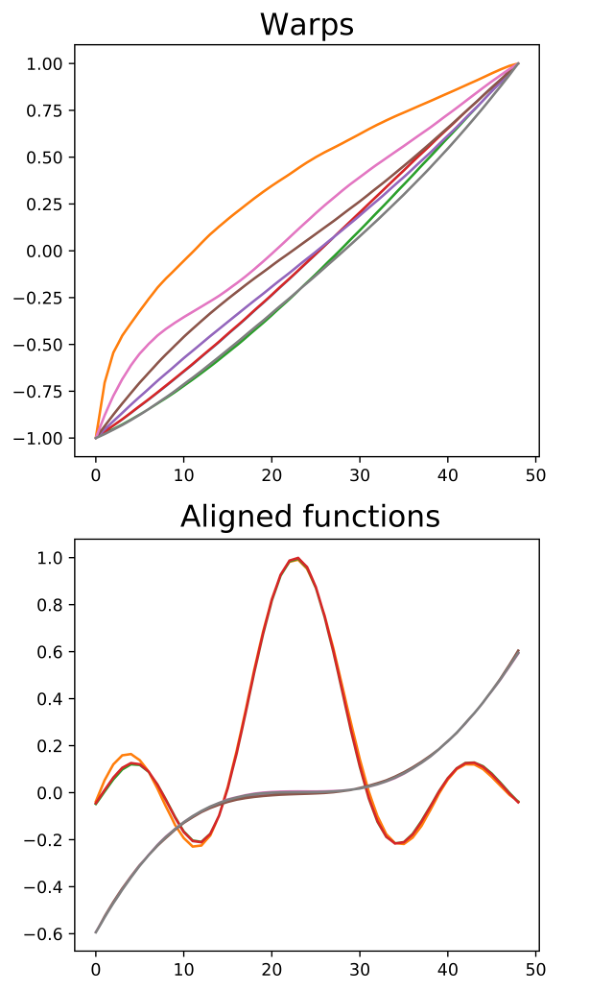
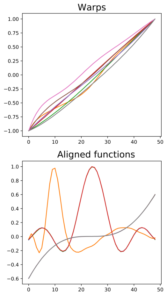
Figure 8: Given noisy observations of warped sequences, we compare the uncertainty in the warps for the proposed model (with and without correlations) and for [Kazlauskaite et al., 2019].
A monotonic constraint in the first layer is desirable in mixed effects models where the first layer corresponds to a warping of space or time that does not allow permutations. We consider an application of the monotonic random process as an integral part of a model designed to align multiple temporal sequences of observations. This problem is introduced in detail in [Kazlauskaite et al., 2019] and here we provide a short summary and the baseline model. We change notation to match [Kazlauskaite et al., 2019]; for the alignment application, refers to the monotonic function, specified using the monotonic Gaussian process flow model, whereas is now an arbitrary function.
Assume we are given some time-series data with inputs and output sequences . We know that there are multiple underlying functions that generated this data, say such functions, , and the observed data were generated by warping the temporal inputs to the true functions using a monotonic warping function , such that:
| (6) |
where is observation noise. Then the corresponding, latent, sequences that are not corrupted by the temporal warp (i.e. the aligned versions of ) are . The functions are modelled jointly using a GP and the joint conditional likelihood for each pair of sequences, and , is:
| (7) | ||||
where are finite-dimensional realisations of the warping function, and includes the parameters of the GP that models function and the parameters of the warping function . The task is then to learn the latent functions and the warps such that the versions of these function which are not corrupted by the warp, , are aligned as well as possible. Note that the number of distinct functions is unknown must also be inferred from the data. This is achieved by formulating an alignment objective that pushes the uncorrupted sequences into groups where each group corresponds to one latent function , and the sequences within each group are aligned to each other. If the warps fully explain the differences between the sequences within each group, then each group contains a single sequence (or, equivalently, all the sequences within a group coincide); see Fig. 4.
Previously, [Kazlauskaite et al., 2019] proposed a probabilistic alignment objective based on a GP latent variable model (GP-LVM) [Lawrence, 2004] that aligns sequences within groups. A GP-LVM is a generative model that is often used as a dimensionality reduction technique to uncovers the latent structure in the data by constructing a low dimensional manifold, and using independent GPs as mappings from a latent space to an observed space. In a GP-LVM, GPs are taken to be independent across the features (columns) of the data , and the likelihood function is:
| (8) |
where are the latent variables for each sequence, the GP covariance is and is a noise precision. Typically, a GP-LVM contains a prior on the latent variables . This encourages the latent variables to be placed close to the origin in the latent space if the observed data can be explained by a single cluster in a latent space; otherwise a minimal number of clusters of in the latent space will be made under the Bayesian prior encouraging sparsity. Furthermore, the stationary kernel in the GPs that map from the latent space to the observed space depend only on the distance between the latent location , which means that the further each latent location is from the others, the less correlated the corresponding GP outputs . Specifically, this behaviour is controlled by the kernel length-scale which allows to reduce correlation between groups of sequences while maintaining strong correlation among sequences within each group.
The two objectives of (7) and (8) are combined to learn the GPs for , the warps and the number of underlying clusters . The baseline [Kazlauskaite et al., 2019] uses MAP estimates for the fitting of the GPs in (7) and for the GP-LVM in (8). This leads to point estimates of the warps and, consequently, does not retain any information about the uncertainty of cluster assignments. Fig. 5 illustrates the limitation of using point estimates; the observed data can be explained in multiple different ways which cannot be uncovered using point estimates.
Uncertainty in monotonic warps
We demonstrate the ability of our monotonic random process to capture the uncertainties in the warps and the cluster assignments in the alignment model. In order to preserve the compositional uncertainty in both the warping functions and the latent functions , we introduce correlations between the variational distributions in the two layers, and using the inference scheme detailed in [Ustyuzhaninov et al., 2019]. Fig. 8 illustrates this phenomenon, and compares the uncertainty in the warps for the original point estimate [Kazlauskaite et al., 2019], the monotonic flow and the flow with correlations between the samples from the warp and the function . The flow captures a range of different possible warpings that are consistent with our prior (which favours solutions that are close to an identity warp) and also fits and aligns the data well. An additional example with bi-modal behaviour, as in Fig. 5, is given in Fig. A1 in the Supplement.
7 CONCLUSION
We have proposed a novel nonparametric model of monotonic functions based on a random process with monotonic trajectories that confers improved performance over the state-of-the-art as well as preferable theoretical properties. Many real-life regression tasks deal with functions that are known to be monotonic, and explicitly imposing this constraint helps uncover the structure in the data, especially when the observations are noisy or data are scarce. We have also demonstrated that the proposed construction can be used as part of a complex alignment model where the uncertainty estimates provide a more informative model and help uncover structures in the data that are not captured by the existing models. More broadly, with additional mid-hierarchy marginal information or domain specific knowledge of compositional priors, e.g. [Kaiser et al., 2018], hierarchical models may necessitate a composition of (injective) monotonic mappings for all but the output layer. This advocates the study of monotonic functions, which can represent a wide variety of transformations and hence serve as a general purpose first layer in a hierarchical model, especially, when the function is known to be non-stationary.
Acknowledgments
This work has been supported by EPSRC CDE (EP/L016540/1) and CAMERA (EP/M023281/1) grants as well as the Royal Society. The authors are grateful to Markus Kaiser and Garoe Dorta for their insight and feedback on this work, and to Michael Andersen for sharing the implementation of Transformed GPs. IK would like to thank the Frostbite Physics team at EA.
References
- [Abadi et al., 2015] Abadi, M., Agarwal, A., Barham, P., Brevdo, E., Chen, Z., Citro, C., Corrado, G. S., Davis, A., Dean, J., Devin, M., Ghemawat, S., Goodfellow, I., Harp, A., Irving, G., Isard, M., Jia, Y., Jozefowicz, R., Kaiser, L., Kudlur, M., Levenberg, J., Mané, D., Monga, R., Moore, S., Murray, D., Olah, C., Schuster, M., Shlens, J., Steiner, B., Sutskever, I., Talwar, K., Tucker, P., Vanhoucke, V., Vasudevan, V., Viégas, F., Vinyals, O., Warden, P., Wattenberg, M., Wicke, M., Yu, Y., and Zheng, X. (2015). TensorFlow: Large-Scale Machine Learning on Heterogeneous Systems. Software available from tensorflow.org.
- [Andersen et al., 2018] Andersen, M. R., Siivola, E., Riutort-Mayol, G., and Vehtari, A. (2018). A non-parametric probabilistic model for monotonic functions. “All Of Bayesian Nonparametrics” Workshop at NeurIPS.
- [Bornkamp and Ickstadt, 2009] Bornkamp, B. and Ickstadt, K. (2009). Bayesian nonparametric estimation of continuous monotone functions with applications to dose-response analysis. Biometrics, 65(1):198–205.
- [Canini et al., 2016] Canini, K., Cotter, A., Gupta, M., Milani Fard, M., and Pfeifer, J. (2016). Fast and flexible monotonic functions with ensembles of lattices. In Advances in Neural Information Processing Systems (NeurIPS).
- [Chen et al., 2018] Chen, R., Rubanova, Y., Bettencourt, J., and Duvenaud, D. (2018). Neural ordinary differential equations. In Advances in Neural Information Processing Systems (NeurIPS).
- [Curtis and Ghosh, 2011] Curtis, S. M. and Ghosh, S. K. (2011). A variable selection approach to monotonic regression with bernstein polynomials. Journal of Applied Statistics, 38(5):961–976.
- [Da Veiga and Marrel, 2012] Da Veiga, S. and Marrel, A. (2012). Gaussian process modeling with inequality constraints. Annales de la Faculté des sciences de Toulouse : Mathématiques, Ser. 6, 21(3):529–555.
- [Dette and Scheder, 2006] Dette, H. and Scheder, R. (2006). Strictly monotone and smooth nonparametric regression for two or more variables. Canadian Journal of Statistics, 34(4):535–561.
- [Durot and Lopuhaä, 2018] Durot, C. and Lopuhaä, H. (2018). Limit theory in monotone function estimation. Statistical Science, 33(4):547–567.
- [Foong et al., 2019] Foong, A. Y. K., Burt, D. R., Li, Y., and Turner, R. E. (2019). Pathologies of factorised gaussian and mc dropout posteriors in bayesian neural networks.
- [Golchi et al., 2015] Golchi, S., Bingham, D., Chipman, H., and Campbell, D. (2015). Monotone emulation of computer experiments. SIAM-ASA Journal on Uncertainty Quantification, 3(1):370–392.
- [Hall and Huang, 2001] Hall, P. and Huang, L.-S. (2001). Nonparametric kernel regression subject to monotonicity constraints. Annals of Statistics, 29(3):624–647.
- [Haslett and Parnell, 2008] Haslett, J. and Parnell, A. (2008). A simple monotone process with application to radiocarbon-dated depth chronologies. Journal of the Royal Statistical Society. Series C, 57:399–418.
- [Hegde et al., 2019] Hegde, P., Heinonen, M., Lähdesmäki, H., and Kaski, S. (2019). Deep learning with differential gaussian process flows. In International Conference on Artificial Intelligence and Statistics (AISTATS).
- [Heinonen et al., 2018] Heinonen, M., Yildiz, C., Mannerström, H., Intosalmi, J., and Lähdesmäki, H. (2018). Learning unknown ode models with gaussian processes. In International Conference on Machine Learning (ICML).
- [Kaiser et al., 2018] Kaiser, M., Otte, C., Runkler, T., and Ek, C. H. (2018). Bayesian alignments of warped multi-output gaussian processes. In Advances in Neural Information Processing Systems (NeurIPS).
- [Kazlauskaite et al., 2019] Kazlauskaite, I., Ek, C. H., and Campbell, N. (2019). Gaussian process latent variable alignment learning. In International Conference on Artificial Intelligence and Statistics (AISTATS). PMLR.
- [Kim et al., 2018] Kim, D., Ryu, H., and Kim, Y. (2018). Nonparametric bayesian modeling for monotonicity in catch ratio. Communications in Statistics: Simulation and Computation, 47(4):1056–1065.
- [Lavine and Mockus, 1995] Lavine, M. and Mockus, A. (1995). A nonparametric bayes method for isotonic regression. Journal of Statistical Planning and Inference, 46(2):235–248.
- [Lawrence, 2004] Lawrence, N. D. (2004). Gaussian process latent variable models for visualisation of high dimensional data. Advances in neural information processing systems, 16(3):329–336.
- [Lenk and Choi, 2017] Lenk, P. and Choi, T. (2017). Bayesian analysis of shape-restricted functions using gaussian process priors. Statistica Sinica, 27(1):43–69.
- [Lin and Dunson, 2014] Lin, L. and Dunson, D. (2014). Bayesian monotone regression using gaussian process projection. Biometrika, 101(2):303–317.
- [Lopez-Lopera et al., 2019] Lopez-Lopera, A. F., John, S., and Durrande, N. (2019). Gaussian process modulated cox processes under linear inequality constraints. In International Conference on Artificial Intelligence and Statistics (AISTATS).
- [Lorenzi et al., 2019] Lorenzi, M., Filippone, M., Frisoni, G., Alexander, D., and Ourselin, S. (2019). Probabilistic disease progression modeling to characterize diagnostic uncertainty: Application to staging and prediction in alzheimer’s disease. NeuroImage, 190:56–68.
- [Maatouk, 2017] Maatouk, H. (2017). Finite-dimensional approximation of gaussian processes with inequality constraints. arXiv:1706.02178.
- [Nader et al., 2019] Nader, C. A., Ayache, N., Robert, P., and Lorenzi, M. (2019). Monotonic gaussian process for spatio-temporal trajectory separation in brain imaging data. arXiv:1902.10952.
- [Øksendal, 1992] Øksendal, B. (1992). Stochastic Differential Equations (3rd Ed.): An Introduction with Applications. Springer-Verlag.
- [Raket et al., 2016] Raket, L. L., Grimme, B., Schöner, G., Igel, C., and Markussen, B. (2016). Separating timing, movement conditions and individual differences in the analysis of human movement. PLOS Computational Biology, 12(9):1–27.
- [Ramsay, 1988] Ramsay, J. (1988). Monotone regression splines in action. Statistical Science, 3(4):425–441.
- [Ramsay, 1998] Ramsay, J. (1998). Estimating smooth monotone functions. Journal of the Royal Statistical Society. Series B, 60(2):365–375.
- [Rasmussen and Williams, 2005] Rasmussen, C. E. and Williams, C. K. I. (2005). Gaussian Processes for Machine Learning.
- [Riihimäki and Vehtari, 2010] Riihimäki, J. and Vehtari, A. (2010). Gaussian processes with monotonicity information. International Conference on Artificial Intelligence and Statistics (AISTATS).
- [Shively et al., 2009] Shively, T. S., Sager, T. W., and Walker, S. G. (2009). A bayesian approach to nonparametric monotone function estimation. Journal of the Royal Statistical Society: Series B (Statistical Methodology), 71(1):159–175.
- [Siivola et al., 2016] Siivola, E., Piironen, J., and Vehtari, A. (2016). Automatic monotonicity detection for gaussian processes. arXiv:1610.05440.
- [Sill and Abu-Mostafa, 1997] Sill, J. and Abu-Mostafa, Y. (1997). Monotonicity hints. In Advances in Neural Information Processing Systems (NeurIPS).
- [Snoek et al., 2014] Snoek, J., Swersky, K., Zemel, R., and Adams, R. (2014). Input warping for bayesian optimization of non-stationary functions. In International Conference on Machine Learning (ICML).
- [Spengler, 1984] Spengler, E. (1984). Ghostbusters.
- [Titsias, 2009] Titsias, M. (2009). Variational Learning of Inducing Variables in Sparse Gaussian Processes. In International Conference on Artificial Intelligence and Statistics (AISTATS).
- [Ustyuzhaninov et al., 2019] Ustyuzhaninov, I., Kazlauskaite, I., Kaiser, M., Bodin, E., Campbell, N. D. F., and Ek, C. H. (2019). Compositional uncertainty in deep gaussian processes. In Bayesian Deep Learning Workshop at NeurIPS.
- [Wahba, 1978] Wahba, G. (1978). Improper priors, spline smoothing and the problem of guarding against model errors in regression. Journal of the Royal Statistical Society. Series B, 49.
- [Wolberg and Alfy, 2002] Wolberg, G. and Alfy, I. (2002). An energy-minimization framework for monotonic cubic spline interpolation. Journal of Computational and Applied Mathematics, 143(2):145–188.
- [Yildiz et al., 2018a] Yildiz, C., Heinonen, M., Intosalmi, J., Mannerstrom, H., and Lahdesmaki, H. (2018a). Learning stochastic differential equations with gaussian processes without gradient matching. In IEEE International Workshop on Machine Learning for Signal Processing (MLSP).
- [Yildiz et al., 2018b] Yildiz, C., Heinonen, M., and Lähdesmäki, H. (2018b). A nonparametric spatio-temporal SDE model. In Spatiotemporal Workshop at NeurIPS.
Supplementary material
A.1 Numerical solution of the SDE
To ensure that the SDE solutions are monotonic functions of the initial values, we make assumptions about the Wiener process realisations . To compute the SDE solutions under such assumptions, we draw a Wiener process realisation as well as the flow field drift and diffusion, and given these draws, we use the Euler-Maryama numerical solver (following [Hegde et al., 2019]). Specifically, starting with the initial state , we use (2) to compute the drift and diffusion at the current state, and the discretised version of (1) (i.e. with and instead of and ) to compute the state update . This gives the new state , and repeating this procedure times, we arrive at the state , corresponding to the approximate SDE solution at time T. The monotonic trajectories are recovered by the numerical SDE solver in the limit of the step size going to zero, . Therefore, the step size must be sufficiently small w.r.t. the smoothness of the flow; since we use a GP to define the flow, the smoothness is determined by the lengthscale of the kernel.
A.2 Implementation details
Our model is implemented in Tensorflow [Abadi et al., 2015]. For the evaluations in Tables 1 and 2 we use iterations with the learning rate of that gets reduced by a factor of when the objective does not improve for more than iterations. For numerical solutions of SDE, we use Euler-Maruyama solver with time steps, as proposed in [Hegde et al., 2019].
A.3 Computational complexity
Computational complexity of drawing a sample from the monotonic flow model is , where is the number of steps in numerical computation of the approximate SDE solution, is the complexity of computing the GP posterior for inputs based on inducing points, and is the complexity of drawing a sample from this posterior. We typically draw fewer than samples to limit the computational cost.
A.4 Non-Gaussian noise
The inference procedures for the monotonic flow and for the 2-layer model can be easily applied to arbitrary likelihoods, because they are based on stochastic variational inference and do not require the closed form integrals of the likelihood density.
A.5 Functions for evaluating the monotonic flow model
The functions we use for evaluations are the following:
-
(flat function)
-
(sinusoidal function)
-
(step function)
-
(linear function)
-
(exponential function)
-
(logistic function)
For the experiments shown in Fig. 3 we generate data points using for linearly spaced inputs .
A.6 Regression evaluation parameters
For the GP with monotonicity information we choose virtual points and place them equidistantly in the range of the data; we provide the best RMSEs for . For the transformed GP we report the best results for the boundary conditions and the number of terms in the approximation . For both models we use a squared exponential kernel. Our method depends on the time , the kernel and the number of inducing points . For this experiment, we consider , and two kernel options, squared exponential and ARD Matérn . The lowest RMSE are achieved using the flow and the transformed GP.
A.7 Uncertainty in alignment model
To further illustrate the advantages of capturing the uncertainty about the warpings, we wish to find the possibly bi-modal warpings for each sequence. We use a Gaussian mixture model (instead of a single Gaussian) as the distribution of both, the warpings and the latent variables in the GP-LVM. In particular, the inducing points of the flow for each sequence are defined to be distributed as a mixture of two multivariate Gaussians. Then, given a draw from the Categorical distribution of this mixture, we defines the clusters assignments for each sample, and assign the resulting aligned sequences to one of the coherent mixture component in the distribution of the latent points of the GP-LVM. Fig. A1 illustrates this behaviour, and gives an example where the uncertainty in the warps results in ambiguity in cluster assignments. A full discussion of the importance of correlations in the variational parameters for compositional uncertainty is available in [Ustyuzhaninov et al., 2019] which provides further details of the inference scheme used.


A.8 Quantitative results
The expected log posterior predictive density is an evaluation metric defined as:
| (9) | ||||
The results on the data described in Sec. 5 (with 100 data points) for the GP with derivatives [Riihimäki and Vehtari, 2010], the transformed GP [Andersen et al., 2018] and the monotonic flow are given in Table 3.
flat sinusoidal step linear exponential logistic GP 15.1 21.9 27.1 16.7 19.7 25.5 GP projection [Lin and Dunson, 2014] 11.3 21.1 25.3 16.3 19.1 22.4 Regression splines [Shively et al., 2009] 9.7 22.9 28.5 24.0 21.3 19.4 GP approximation [Maatouk, 2017] 8.2 20.6 41.1 15.8 20.8 21.0 GP with derivatives [Riihimäki and Vehtari, 2010] 16.5 5.1 19.9 2.9 68.6 5.5 16.3 7.6 27.4 6.5 30.1 5.7 Transformed GP [Andersen et al., 2018] (VI-full) 6.4 4.5 20.6 5.9 52.5 3.6 11.6 5.8 17.5 7.3 17.1 6.2 Monotonic Flow (ours) 6.8 3.2 17.9 4.2 20.5 5.0 13.2 6.7 14.4 4.8 18.1 5.0
flat sinusoidal step linear exponential logistic Transformed GP [Andersen et al., 2018] (VI-full) 18.5 14.4 40.0 17.5 101.9 11.4 37.4 22.8 52.9 11.9 51.7 19.6 Monotonic Flow (ours) 21.7 15.0 39.1 13.0 64.5 10.7 30.8 12.0 32.8 17.9 43.2 15.2
flat sinusoidal step linear exponential logistic GP with derivatives [Riihimäki and Vehtari, 2010] -1.43 0.08 -1.41 0.06 -1.69 0.15 -1.36 0.04 -1.45 0.08 -1.45 0.11 Transformed GP [Andersen et al., 2018] (VI-full) -1.44 0.03 -1.39 0.02 -1.51 0.06 -1.40 0.03 -1.41 0.02 -1.41 0.02 Monotonic Flow (ours) -1.39 0.05 -1.42 0.05 -1.41 0.08 -1.39 0.05 -1.40 0.07 -1.43 0.07