The Curious Case of Leading Transcendentality: three-point Form FactorsPreprint: IMSc/2019/0506, MPP-2019-100, PSI-PR-19-10
Abstract
Form factors are important ingredients to investigate the principle of maximal transcendentality (PMT) and to extract anomalous dimensions of local gauge invariant operators. In this article, we compute several two- and three-point FFs to three- and two-loops, respectively, for three different choices of local gauge invariant operators in super Yang-Mills (SYM) theory. The operators and are flavour and helicity blind configurations of supersymmetric descendant of the half-BPS and Konishi primary, respectively, and is the energy-momentum tensor. The operators and are composed of non-protected dimension-three (classical) fermionic and scalar components belonging to SU() closed sub-sector of SYM. We analyse the mixing among the non-protected fermionic and scalar components of these operators up to three-loops in perturbation theory and consequently, compute the quantum corrections to the corresponding dilatation operators. The highest transcendental (HT) weight terms of the FFs of are found to be independent of the external on-shell states and, moreover, those are equal to that of half-BPS, however, this does not hold true for the FFs of . FFs of the exhibit identical behaviours to that of half-BPS, in concordance with the classical expectations. However, the three-point FFs of violate the PMT while comparing with the corresponding quantity in the standard model, observed for the first time at the level of FF.
Keywords
Maximally SYM, form factor, three-point, principle of maximal transcendentality.1 Introduction
On-shell scattering amplitudes and off-shell correlation functions are quantities of fundamental importance in any gauge theory. A generic quantum field theory is completely specified by the knowledge of these quantities. Form factors (FFs), the overlap of an -particle on-shell state with a state created by the action of a local gauge invariant operator on the vacuum, are a fascinating bridge between aforementioned two quantities which have been studied extensively in quantum chromodynamics (QCD) and super Yang-Mills (SYM) theory:
| (1) |
The numbers denote the on-shell particles and is the off-shell momentum associated with the operator. The central objects which are considered in this article are two- and three-point FFs. Very recently, the first calculations of generalisations of such FFs to the case of two operator insertions with one non-protected operator was performed Ahmed:2019upm by some of us.
In this work, we begin our discussion by considering two local gauge invariant operators:
| (2) |
The Majorana and scalar fields are denoted through and , respectively. All the fields in SYM transform under the adjoint representation of SU(N) gauge group which is captured through the indices with . The Yang-Mills coupling strength is denoted by . Four generations of Majorana fermions are represented through . The indices denote the generation number of scalar and pseudo-scalar fields with in 4-dimensions. The fully anti-symmetric structure constants of SU(N) group is defined through . The aforementioned operators in (1) are constructed out of non-protected, dimension-three (classical) fermionic and scalar components which belong to SU closed subsector of SYM. The FFs in this sector were first studied in ref. Brandhuber:2016fni. The helicity and flavour dependent counterparts of the operator was obtained Intriligator:1999ff; Bianchi:2001cm; Beisert:2003ys as conformal descendant of the half-BPS and the was obtained as supersymmetric descendant of Konishi primary Eden:2005ve; Brandhuber:2016fni.
Understanding the mathematical structures of scattering amplitudes and FFs in SYM has been an active area of investigation for past several decades, not only due to its underlying ultraviolet conformal symmetry but also its ability to help in solving more complicated theory like QCD. One of the most interesting facts is the presence of uniform transcendental11 1 The weight of transcendentality, , of a function, , is defined as the number of iterated integrals required to define the function , e.g. and also we define . Algebraic factors are assigned weight zero and dimensional regularisation parameter to -1. (UT) terms in certain class of scattering amplitudes and FFs in SYM. This is indeed an observational Kotikov:2002ab; Kotikov:2004er; Bern:2006ew; Drummond:2007cf; Naculich:2008ys; Bork:2010wf; Gehrmann:2011xn; Brandhuber:2012vm; Eden:2012rr; Drummond:2013nda; Basso:2015eqa; Ahmed:2016vgl; Goncalves:2016vir; Banerjee:2016kri; Banerjee:2018yrn, albeit unproven, fact. The two-point or Sudakov FFs of the half-BPS operator belonging to the stress-energy supermultiplet is found vanNeerven:1985ja; Brandhuber:2010ad; Gehrmann:2011xn to contain terms with UT, more specifically, they are composed of only highest transcendental (HT) terms with weight 2L at loop order L. It is also shown in ref. Gehrmann:2011xn that it is possible to choose a representation in which each loop integral has uniform transcendentality. This has profound implications in choosing the basis of master integrals while computing Feynman loop integrals through method of differential equation. Therefore, it is very natural to examine how far this behaviour holds true. In light of this, in ref. Brandhuber:2012vm, the three-point FFs of the half-BPS operator are investigated and those are found to respect this wonderful property. On the contrary, this behaviour fails for the Konishi KONISHI1984439, the primary operator for the Konishi supermultiplet, for two- Nandan:2014oga as well as three-point Banerjee:2016kri FFs. All the aforementioned results are in accordance with the general observation that the FFs of supersymmetry (SUSY) protected operators exhibit UT behaviour. However, there is no clear indication whether the reverse is also true. Through our computations, we find that the three-point one-loop FF of operator with on-shell states does not exhibit UT behaviour. However, all the remaining two- and three-point FFs of and do not exhibit UT behaviours.
It is conjectured in ref. Loebbert:2015ova that at two-loop level the HT weight parts of every two-point minimal FF (number of fields present in the operator is same as number of external on-shell states) are identical and those are same as that of half-BPS operator belonging to the stress-energy supermultiplet vanNeerven:1985ja. In ref. Ahmed:2016vgl, this conjecture is verified to three-loops level for the FF of unprotected Konishi operator. In ref. Brandhuber:2014ica, the minimal FFs of long BPS operators (more than two fields) are computed to two-loops, and the corresponding HT piece is found to be a universal in all FFs with long, unprotected operators Loebbert:2015ova; Brandhuber:2016fni; Brandhuber:2017bkg; Jin:2018fak; Jin:2019ile; Brandhuber:2018kqb. The operators in (1) are combination of long and short unprotected parts. Moreover, the corresponding FFs can neither be regarded as minimal nor non-minimal case. This kind of scenario is largely unexplored. Through our computations of three-point FFs, we show that the HT piece of is independent of the external states and it is equal to that of half-BPS Brandhuber:2012vm; Banerjee:2016kri. However, for the operator , this property fails for all the FFs.
It is also conjectured in Loebbert:2015ova, that the HT terms of two-loop remainder function of the three-point FF of every length-two operator should agree with the corresponding half-BPS remainder found in ref. Brandhuber:2012vm. The latter conjecture is falsified in ref. Banerjee:2016kri where, for the first time, it is shown that for three-point FF of the Konishi operator (length-two), the HT part depends on the nature of external on-shell states; it fails to match with that of half-BPS if the external on-shell states are . The operators in (1) are combinations of length-two and three operators. As mentioned in the previous paragraph, though the HT parts of the three-point FFs are identical to that of half-BPS Brandhuber:2012vm; Banerjee:2016kri, it fails for the FFs of which can be thought of as a general feature of Konishi primary and its descendants.
In past few decades, people have been investigating the connection among quantities computed in different gauge theories. In particular, the connection between on-shell amplitudes or FFs of SYM and that of QCD are of fundamental importance. Besides theoretical understanding, this is motivated from the fact that calculating any quantity in QCD is much more complex and in absence of our ability to calculate a quantity in QCD, whether it is possible to get the result, at least partially, from some other simpler theory. In refs. Kotikov:2001sc; Kotikov:2004er; Kotikov:2006ts, the connection between anomalous dimensions of leading twist-two operators of these theories is found and it is shown that the results in SYM is related to the HT part of the QCD results and consequently, the principle of maximal transcendentality (PMT) is conjectured. Same conclusion is obtained by some of us in Banerjee:2018yrn through a different procedure based on momentum fraction space. At this level, this connection involves only pure number. This property is later examined in the context of two-point FFs in Gehrmann:2011xn to three-loops level and surprisingly, found to hold true: the HT pieces of quark (vector interaction) and gluon (scalar interaction) FFs in QCD Gehrmann:2011aa are identical to scalar FFs of half-BPS operator in SYM upon changing the representation of fermions in QCD from fundamental to adjoint. The same behaviour is also found for the quark and gluon two-point FFs Ahmed:2015qia; Ahmed:2016qjf associated to tensorial interaction through energy-momentum tensor. In refs. Brandhuber:2012vm; Banerjee:2017faz; Brandhuber:2017bkg; Jin:2018fak; Jin:2019ile, the same behaviour is found to replicate for three-point scalar and pseudo-scalar FFs. This is the first scenario where non-trivial kinematics is involved and the validity of this principle implies this not only holds true for pure numbers but also for functions containing non-trivial kinematic dependence. Even after including the dimension seven operators in the effective theory of Higgs boson in the Standard model, PMT is also found to hold true Jin:2018fak; Brandhuber:2018xzk; Jin:2019opr for three-point FFs. Using this principle, the four-loop collinear anomalous dimension in planar SYM is determined in ref. Dixon:2017nat. The complete domain of validity of this principle is still not fully clear and it is under active investigation. For on-shell scattering amplitudes, it breaks down even at one loop Bern:1993mq for cases with four or five external gluons. Considering three different operators, in this article, we check the validity of this conjecture for various two- and three-point FFs.
The aforesaid operators in (1) are composed of two parts, one containing two Majorana fields, and the other with three scalar fields. Under quantum corrections, these components mix with each other and develop ultraviolet (UV) poles which manifest as non-zero anomalous dimensions. In order to investigate the mixing and determine the underlying anomalous dimensions, we compute several three-point two-loop and two-point three-loop form factors with the operators and insertions. By exploiting the universality of infrared divergences, we calculate the anomalous dimension matrix for the operator fully up to two-loops and partially at three-loop, and for partially to two-loops. Our findings of are consistent with the partially two-loop results available in ref. Brandhuber:2016fni. The anomalous dimensions of are identical to the Konishi supermultiplet, in accordance with the expectations Eden:2005ve; Brandhuber:2016fni. The anomalous dimensions are the corrections to the corresponding dilatation operators which can provide us non-trivial quantum field theoretic test for integrability.
One of the main motivations for constructing helicity, flavour blind operators in (1), in contrast to the ones considered in refs. Intriligator:1999ff; Bianchi:2001cm; Beisert:2003ys; Eden:2005ve; Eden:2009hz; Brandhuber:2016fni is to compare its FFs with known QCD results available for and amplitudes directly, where stand for the Higgs boson, gluon and bottom quark, respectively.
Energy-momentum tensor (EM), which is also considered in this article, has been studied extensively in the context of three-point FFs in QCD Ahmed:2014gla; Ahmed:2016yox, and is found to behave like the half-BPS at one- as well as two-loop order and it is independent of the associated external on-shell states. This is in accordance with our classical expectation: since the stress-tensor is protected and lies in the same multiplet as the half-BPS, an exact SUSY Ward identity would relate these two FFs. Quite surprisingly, the process with three external partons violates the PMT even at one-loop while comparing the corresponding quantities in QCD! This is observed for the first time at the level of three-point FF.
After an initial introduction to the basics of SYM, we present the explicit form of the EM tensor in section 2. All the processes that are analysed up to two- and three-loops level are also tabulated in the same section. In the following section 2.1, we define the FFs and relate those with underlying scattering matrix elements. The methodology of the computation is briefly discussed in section 2.2. In this article, we use the Feynman diagrammatic approach, in contrast to popular on-shell unitarity methods in the context of SYM, along with the integration-by-parts Tkachov:1981wb; Chetyrkin:1981qh identities. Though SYM is ultraviolet finite, that manifests through the vanishing -function, nevertheless we need to regularise the theory not only because of the presence of soft and collinear divergences, but also due to appearance of non-zero anomalous dimensions for unprotected operators. In order to see these divergences explicitly and make sense out of the quantities we are interested in, we regularise the theory using modified dimensional reduction () Siegel:1979wq; Capper:1979ns which is discussed in section 3. In the presence of unprotected operators, the method to perform UV renormalisation is discussed in section 3.1. The universal behaviour of infrared (soft and collinear) divergences is described in section 3.2. In section 3.3, the mixing among the constituent operators due to quantum corrections is demonstrated. In addition to calculating the finite FFs following Catani’s subtraction scheme, we also compute finite remainders which is introduced in section 4. The behaviour of the FFs in the light of UT and PMT is analysed in details in section 5 which encapsulates many interesting findings. We also perform several consistency checks, discussed in section 7, analytical as well as numerical to increase the reliability of our results. Concluding remarks are made in the last section 8. In the appendix A, we give explicit analytic results of all the FFs.
2 Theoretical framework
The dynamics of SYM is encapsulated through the Lagrangian density Brink:1976bc; Gliozzi:1976qd; Jones:1977zr; Poggio:1977ma
| (3) |
The gauge, ghost, Majorana, scalar and pseudo-scalar fields are denoted through and , respectively. represents the field strength tensor that is related to the gauge field through covariant derivate . All the fields in SYM transform under the adjoint representation of SU(N) gauge group which is captured through the indices with . The Yang-Mills coupling strength is denoted by and is the gauge fixing parameter. Four generations of Majorana fermions are represented through . The indices denote the generation numbers of scalar and pseudo-scalar fields with in 4-dimensions. The fully anti-symmetric structure constants of SU(N) group is defined through . and are anti-symmetric matrices satisfying the SUSY algebra:
| (4) |
| (5) |
In this article, in addition to considering the operators and defined in (1), we also consider the energy-momentum tensor which reads
| (6) |
This operator was considered in ref. Banerjee:2018yrn in computing all the splitting functions in SYM. We are interested in two- and three-point form factors to three- and two-loops, respectively, consisting of a colourless off-shell state (), described by the insertion of a local gauge invariant operator
| (7) |
where and are the corresponding 4-momentum with . The outgoing on-shell particles are denoted by . In this article, we consider several processes which are
| (8) | ||||
| (9) | ||||
| (10) | ||||
| (11) |
The underlying Lagrangian density encapsulating the interaction of the off-shell states described by gauge invariant local operators, defined in (1), to the fundamental fields of SYM is given by
| (12) |
So, the full underlying Lagrangian for the scattering processes under consideration reads
| (13) |
We define the kinematic invariants of the processes through
| (14) |
satisfying . We also introduce dimensionless invariants out of these as
| (15) |
which satisfies the constraint . All the results are presented in terms of Multiple Polylogarithms (MPLs) goncharov1998multiple; goncharov2001multiple containing these parameters. In the next section, we define the form factors in terms of matrix elements.
2.1 Two- and three-point form factors
In perturbation theory, any scattering amplitude can be expressed as expansion in powers of coupling constant
| (16) |
where the quantity represents the -th loop amplitude of the scattering process depicted in (7). The expansion parameter, , is the ’t Hooft coupling Bern:2005iz given by
| (17) |
with the Euler constant . is the quadratic Casimir of SU(N) group in adjoint representation. in (16) corresponds to the power of coupling constant of the leading order amplitude. Form factors are constructed out of the transition matrix elements through
| (18) |
The goal of this article is to calculate the three-point FFs to two-loops i.e. , for the processes in (9), (10), (11), and two-point FFs up to three-loops i.e. , , for the processes in (8). In the next section, we discuss the methodology of the computations.
2.2 Methodology of the computation
In spite of the presence of many modern techniques bases on unitarity, Feynman diagrammatic approach of evaluating loop amplitudes remains a potential candidate which is employed in this article. We begin by generating the Feynman diagrams of a process using QGRAF Nogueira:1991ex. Because of the presence of Majorana fermions which destroy the flow of fermionic current, a special care needs to be taken. We use a code22 2 We thank Satyajit Seth for the Python code. based on PYTHON to rectify it which is further processed through a series of in-house FORM Vermaseren:2000nd routines in order to apply the Feynman rules, perform Dirac, Lorentz and SU(N) color algebras. To ensure the inclusion of only physical states of the gauge fields, we take into account the ghost loops for internal states and the polarisation sum of the external gluons is performed in axial gauge. For the tensorial interaction, the polarisation sum in dimensions reads Mathews:2004xp
| (19) |
Besides the complicated terms in tensorial operator in (2), the presence of several terms in polarisation sum in (2.2) makes the calculation worse by surging the size of the expression substantially. After performing the Dirac and Lorentz algebras in dimensions and contracting all the indices, the Feynman diagrams manifest as scalar integrals in dimensions. Using the liberty of transforming loop momentum, with the help of REDUZE2 vonManteuffel:2012np; Studerus:2009ye, we categorise all the scalar integrals into 3- and 6-integral families Ahmed:2014gla; Ahmed:2014pka at one- and two-loop, respectively. All the scalar integrals are later related to a much smaller set of master integrals (MIs) through integration-by-parts (IBP) Tkachov:1981wb; Chetyrkin:1981qh and Lorentz invariant (LI) Gehrmann:1999as identities. We use LiteRed Lee:2008tj; Lee:2012cn along with Mint Lee:2013hzt to perform the integral reduction which ultimately relates all the scalar integrals to 7 and 89 MIs at one- and two-loop, respectively whose results are available in Gehrmann:2000zt; Gehrmann:2001ck. The results are expressed in terms of harmonic polylogarithms (HPLs) Gehrmann:1999as and two-dimensional HPLs (2dHPLs) Gehrmann:2000zt; Gehrmann:2001ck; Gehrmann:2001jv. Using the results of the MIs, we get all the FFs to two-loops which are presented explicitly in the appendix A. In the next section, we discuss the regularisation procedure, operator renormalisation and infrared factorisation.
3 Regularisation prescription and renormalisations
The SYM is one of the few ultraviolet finite quantum field theories in 4 space-time dimensions. The on-shell amplitudes and FFs of protected operators are guaranteed to be UV finite. However, unprotected operators do develop divergences arising from the UV sector owing to the short distance effects which gets reflected through the presence of non-zero UV anomalous dimensions. Besides, due to the presence of massless vertices in the Lagrangian, the theory is not soft and collinear (IR) finite. Consequently, the on-shell amplitudes as well as FFs involve IR divergences. To identify these divergences, we need to regularise the theory following appropriate prescription. In this article, we adopt supersymmetry preserving modified dimensional reduction () scheme Siegel:1979wq; Capper:1979ns where the bosonic and fermionic degrees of freedom (DOF) are maintained to be equal throughout the calculation. In order to achieve that the number of scalar and pseudo-scalar generations are changed from to in dimensions. The Majorana fermions are remained to have 4 generations. Together with DOF of gauge fields in dimensions, the total bosonic DOF equals 8 which is same as that of fermions, consequently the SUSY remains intact. The Dirac algebra and the traces of matrices, being dependent on the generation number of the scalar and pseudo-scalar fields, are performed in dimensions which obey
| (20) |
The denotes 4x4 identity matrix. In the next section, we discuss about the UV renormalisation.
3.1 UV renormalisation
The on-shell amplitudes in SYM does not suffer from UV singularities owing to the vanishing of -functions to all orders in perturbation theory. However, the FFs of an unprotected composite operator may develop UV divergences which can be manifested by the presence of non-zero UV anomalous dimensions in the FFs beyond leading order. Thus, any FF involving an unprotected operator needs to go through UV renormalisation which is performed by multiplying an overall operator renormalisation constant, , defined through
| (21) |
The UV anomalous dimensions of the operator are denoted through . This is a property inherently associated to the operator itself, it does not depend upon the nature of on-shell states. In particular, the bare operator, , gets renormalised through
| (22) |
The quantities can be determined by exploiting the universal infrared structures of the two- and three-point FFs and solving the underlying renormalisation group equation satisfied by Ahmed:2015qpa; Banerjee:2018yrn. In section. 3.3, we discuss the computation of operator renormalisation constants for the operators and . Being conserved to all orders, the is identically equal to 1. The scale appearing in (21) is introduced through
| (23) |
where, is the coupling constant appeared in the regularised Lagrangian in dimensions and is the scale introduced to make dimensionless.
The UV renormalised matrix elements can be expanded in powers of bare as well as renormalised coupling through
| (24) |
where the hat signifies the unrenormalised quantities. The quantity for three-point and for two-point FFs. This, in turn, leads us to the expressions of renormalised matrix elements in terms of bare ones order by order in coupling constant. Employing these relations in (18), we determine the UV renormalised FFs at 1-, 2- and 3-loop which are computed in this article. Now we turn our focus towards the infrared factorisation of the FFs.
3.2 Infrared factorisation
Being a massless theory, the UV renormalised FFs exhibit infrared divergences (IR) from soft and collinear configurations. These appear as poles in dimensional regularisation parameter , whose universal nature was first demonstrated in Catani:1998bh. In Sterman:2002qn, a detailed derivation was presented by exploiting the factorisation and resummation properties of scattering amplitudes which was later generalised to all orders in Becher:2009cu; Gardi:2009qi. The IR divergences can be factored out from UV renormalised quantities through the subtraction operators which up to two-loops read
| (25) |
The subtraction operators are independent of the nature of operator insertion, it solely depends on the SU(N) coloured particles. In case of SYM where all the fundamental particles transform under the adjoint representation of SU(N) gauge group and coefficients of -function vanishes to all orders, these take the form
| (26) |
with Becher:2009cu
| (27) |
The arbitrariness of the finite parts of the subtraction operators define various schemes in which finite part of amplitude is computed. Upon translating the infrared factorisation from amplitudes to the UV renormalised FFs depicted in (18), we get exactly same relations as (3.2):
| (28) |
The infrared structure of the Sudakov FF at three-loop can be obtained by solving the renormalisation group equation satisfied by the Sudakov FF Sudakov:1954sw; Mueller:1979ih; Collins:1980ih; Sen:1981sd. Using the solution depicted in refs. Ravindran:2005vv; Ravindran:2006cg; Moch:2005tm, we obtain the universal infrared structures (See ref. Ahmed:2016vgl). Computation of the finite quantities , and is the primary objective of this article. The finite parts of the FFs appearing on the right side of the (3.2) can be organised according to their transcendental weights as
| (29) |
The explicit results of the FFs in terms of MPLs are presented in the appendix A by setting . In the following section, we discuss the operator mixing in the context of operator renormalisation.
3.3 Operator mixing and dilatation operator to three-loops in SU() sector
The operators for are composed of bosonic and fermionic parts which we denote as and , respectively and those are defined through
| (30) |
These constituents operators and mix among themselves under UV renormalisation through
| (31) |
with the mixing matrix
| (32) |
and . The bare operator is denoted by . The operator renormalisation constant is controlled by the corresponding anomalous dimensions, , through renormalisation group equation (RGE)
| (33) |
The general solution of the RGE up to is obtained as (see the appendix of ref. Ahmed:2017rwl for general method of solving RGE)
| (34) |
where are expanded in powers of as
| (35) |
Using the results of the FFs of the renormalised operators, computed in this article, and by demanding the UV finiteness and universality of the infrared singularities, we have computed the operator renormalisation constants or equivalently, the underlying anomalous dimensions. In order to achieve this, we have employed the methodology prescribed in refs. Ahmed:2015qpa; Ahmed:2016qjf; Banerjee:2018yrn. The one-loop results are found to be
| (36) |
From the aforementioned results of the anomalous dimensions, we observe that the diagonal elements, namely, and for the two operators are identical. At two-loop, the results of the anomalous dimensions are obtained as
| (37) |
In order to determine the remaining two components of the anomalous dimensions corresponding to the operator , the computations of three-point three-loop or two-point four-loop FFs are required, which are beyond the scope of this article. In addition to determining these quantities to two-loops, by exploiting the three-loop FFs of the operator , we have also determined some of the elements of the three-loop anomalous dimension matrix, which read 33 3 The three-loop anomalous dimensions are dependent on which is defined through . In regularisation scheme, equals which is the coefficient of in the expansion of . is the number of generations of scalar/pseudo-scalar in , as mentioned in 3.
| (38) |
Our findings are consistent with the partially available two-loop results computed in ref. Brandhuber:2016fni. The components at two-loop, and , at three-loop are new results computed for the first time in this article. The anomalous dimensions of are found to be identical to the Konishi supermultiplet, in accordance with the expectations Eden:2005ve; Brandhuber:2016fni. For readers’ convenience, below we present the mixing matrices explicitly, which read
| (39) |
The quantum corrections to the dilatation operators corresponding to the operators and in the SU() sector Beisert:2003ys; Brandhuber:2016fni are defined as
| (40) |
This is essentially the anomalous dimension matrix with a difference of an overall factor of -1. For readers’ convenience, we also present the results of the below
| (41) |
The remaining components need computations which are beyond the scope of this paper. The results of the which were computed partially to two-loops level in ref. Brandhuber:2016fni are consistent with our findings.
Using the results of the mixing matrix, we can get the renormalised operator defined in (22) as
| (42) |
where, the can be directly read from (3.3). Upon substituting the results of the mixing matrix from (3.3), we have seen that both the operators and have non-zero anomalous dimensions. Moreover, the anomalous dimension of the operator turns out to be identical to that of Konishi supermultiplet, in accordance with the expectations Eden:2005ve; Brandhuber:2016fni.
4 Finite remainders at two-loop
For maximally helicity violating (MHV) amplitude in planar SYM, the helicity blind quantity which is obtained by factoring out the tree level amplitude was conjectured to exponentiate in terms of one-loop counter part along with the universal cusp and collinear anomalous dimensions. This is known as BDS/ABDK ansatz Anastasiou:2003kj; Bern:2005iz. However, this ansatz is found to break down for two-loop six-point amplitudes Bern:2008ap; Drummond:2008aq.
Though the IR divergent parts were found to be consistent with the prediction of the ansatz, the finite part was not. Hence, to capture the amount of deviation from the prediction of BDS/ABDK ansatz, a quantity named finite remainder Bern:2008ap; Drummond:2008aq was introduced which is a finite function of dual conformal cross ratios.
Following this line of thought and inspired by the exponentiation of the IR divergences of FFs, the finite remainder function for FFs at two-loop was introduced in ref. Brandhuber:2012vm as
| (43) |
where . Writing a two-loop FF in terms a quantity dictated by BDS/ABDK ansatz plus a finite remainder provides an efficient way of organising the result - the ansatz part captures the IR divergences whereas the remainder encapsulates the finite part in 4-dimensions. Due to the nature of IR divergences of FFs, the and poles cancel between first two terms in (43), By demanding the finiteness of remainder i.e. the vanishing of the remaining and poles, one gets
| (44) |
The other coefficient and can not be fixed uniquely. To maintain a close resemblance with the corresponding quantity of MHV amplitudes, the is assigned a value according to
| (45) |
With the help of Sudakov FF, the remaining constant is found to be Brandhuber:2012vm
| (46) |
and are independent of the nature of operator and number of external legs. The remainder and finite part of the can be related to each other which can be found in Banerjee:2016kri. In this article, we compute the finite remainders for all the processes and operators which are presented explicitly in the appendix A after setting and organising those according to their transcendental weights as
| (47) |
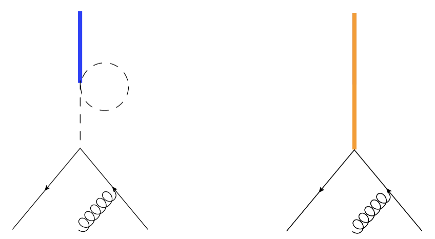
We do not define the finite remainder at two-loop for the processes and due to the involvement of one-loop diagrams arising from . This can be understood by looking at the leading order contributions, shown in figure 1, to these processes which are loop induced through . In the next section, we analyse our results in view of transcendetality weight.
5 Principle of uniform transcendentality
The principle of uniform transcendentality (PUT) is a remarkable feature based on numerous observations Kotikov:2002ab; Kotikov:2004er; Bern:2006ew; Drummond:2007cf; Naculich:2008ys; Bork:2010wf; Gehrmann:2011xn; Brandhuber:2012vm; Eden:2012rr; Drummond:2013nda; Basso:2015eqa; Goncalves:2016vir; Banerjee:2018yrn, albeit unproven, which states that certain kinds of scattering amplitudes and form factors in can be expressed purely in terms of functions having UT. In other words, the L-th loop result is found to contain only polylogarithmic functions of degree 2L. It is conjectured in ref. Loebbert:2015ova that at two-loop level the HT weight parts of every two-point minimal FF (number of fields present in the operator is same as number of external on-shell states) are identical and those are same as that of half-BPS operator belonging to the stress-energy supermultiplet vanNeerven:1985ja. In ref. Brandhuber:2014ica, the minimal FFs of long BPS operators (more than two fields) are computed to two-loops, and the corresponding HT piece is found to be a universal in all FFs with long, unprotected operators Loebbert:2015ova; Brandhuber:2016fni; Brandhuber:2017bkg; Jin:2018fak; Jin:2019ile; Brandhuber:2018kqb. It is also conjectured in Loebbert:2015ova, that the HT terms of two-loop remainder of the three-point FF of every length-two operator should agree with the corresponding half-BPS remainder found in ref. Brandhuber:2012vm which is falsified in ref. Banerjee:2016kri where, for the first time, it is shown that for three-point FF of the Konishi operator (length-two), the HT part depends on the nature of external on-shell states; it fails to match with that of half-BPS if the external on-shell states are . The operator and in (1) are combination of short (length-two) and long (length-three) unprotected parts. Moreover, the corresponding FFs can neither be regarded as minimal nor non-minimal case. So, this scenario does not belong to the domains for which the aforementioned conjectures are made. This kind of scenario is largely unexplored. In this section, we dissect our new results in light of these principles and conjectures, and discuss how far the PUT holds true in present context.
- •
In case of tensorial interaction through operator , for all the processes depicted in (11), the one-loop and two-loop finite parts of the three-point FFs i.e. , in (3.2), are UT. These contain only the HT terms which involve exclusively polylogarithmic functions of transcendentality 2 and 4 at one- and two-loop, respectively. No lower transcendental terms is present. Moreover, the corresponding finite remainder in (43) replicates this behaviour which is exactly similar to the corresponding quantity of the half-BPS operator. More specifically, the results in terms of MPLs are obtained as
(48) where represents terms with transcendentality weight . The above eq. (• ‣ 5) implies that the finite FFs as well as the remainders are independent of the on-shell states. Moreover, the results are exactly same as that of the half-BPS operator Brandhuber:2012vm; Banerjee:2016kri which is presented explicitly in terms of MPLs in appendix A.1. In summary, the energy-momentum tensor behaves exactly like the half-BPS operator at three-point FFs level. This is in accordance with our classical expectation: since the stress-tensor is protected and lies in the same multiplet as the half-BPS, an exact SUSY Ward identity would relate these two FFs.
- •
Through our computations, we find that except the three-point one-loop FF of operator with on-shell states, none of the other two- and three-point FFs of exhibits UT behaviour. The general observation is that the FFs of SUSY protected operators exhibit UT behaviour. However, there is no clear indication whether the reverse is also true. Through the results depicted in (50), we see that the FF of an unprotected operator, such as, can even be UT. The HT parts of the three-point remainder function and the finite FFs at one- as well as two-loop do match with that of half-BPS vanNeerven:1985ja; Gehrmann:2011xn; Brandhuber:2012vm; Banerjee:2016kri:
(49) (50) We also see that the HT terms are independent of the external on-shell states. As expected, the lower transcendental weight terms do depend on the nature of external on-shell states. The results of the aforementioned FFs are presented explicitly in appendix and .
- •
The FFs of the operator have lower transcendental weight terms, similar to that of . However, in contrast to the FFs of , the HT terms of this operator depend on the nature of external on-shell states. Moreover, none of the HT terms of the FFs matches with that of half-BPS:
(51) Similar behaviour in the context of Konishi operator was observed in ref. Banerjee:2016kri for the two-loop three-point FFs with external on-shell states containing . So, we see that the dependence of HT terms on the nature of external on-shell states is a general feature of the FFs of Konishi primary and its descendants.
In ref. Brandhuber:2014ica, the minimal FFs of long BPS operators (more than two fields) are computed to two-loops, and the corresponding HT piece is found to be a universal in all FFs with long (more than two-fields), unprotected operators Loebbert:2015ova; Brandhuber:2016fni; Brandhuber:2017bkg; Jin:2018fak; Jin:2019ile; Brandhuber:2018kqb. For the FF of with the external on-shell states , the one-loop contribution comes only from , the does not contribute at this loop level. So, this one-loop FF effectively comes from a long, unprotected operator. For this case, we see that the HT part of the one-loop FF does not match with the HT term of long BPS operator, and consequently it violates the conjecture.
The results of the FFs of operator are presented explicitly in appendix .
In the following section, we concentrate only on the highest transcendental weight terms and discuss their profound implications.
6 Principle of maximal transcendentality and its violation
The principle of maximal transcendentality (PMT) Kotikov:2001sc; Kotikov:2004er; Kotikov:2006ts establishes a bridge between the results in QCD and those of SYM which are comparatively simpler. It states that for certain quantities, the results in SYM can be obtained from that in QCD by converting the fermions from fundamental to adjoint representation and then retaining only the HT terms. The complete domain of applicability of this principle is still not clear and under active investigation. In this article, we check the applicability of PMT with respect to the operators considered.
For all the FFs of operator and , the HT terms of the finite FFs as well as remainder functions coincide with the corresponding results of the half-BPS operator vanNeerven:1985ja; Gehrmann:2011xn; Brandhuber:2012vm; Banerjee:2016kri, as shown in (• ‣ 5). However, none of the HT parts of the operator matches with that of half-BPS, as shown in (• ‣ 5). In refs. Brandhuber:2012vm; Banerjee:2017faz; Brandhuber:2017bkg; Jin:2018fak; Jin:2019ile, it was shown that the three-point FFs of half-BPS are identical to the HT terms of the quark (vector interaction) and gluon (scalar interaction) FFs of QCD Gehrmann:2011aa after converting the fermions from fundamental to adjoint representation. Consequently, with respect to the quark and gluon FFs in QCD, all of the FFs of and , but , satisfy the PMT.
Now we ask the question, instead of considering the QCD FFs of scalar and vector interactions, if we take the tensorial interaction, does the PMT hold true? Quite remarkably, the answer turns out to be ‘No’: the HT terms of the three-point QCD FFs of EM tensor Ahmed:2014gla; Ahmed:2016yox do not match with the corresponding quantities of SYM upon converting the quarks from fundamental to adjoint representation. To demonstrate this, we consider the processes depicted in (11) in SYM and the corresponding two processes in massless QCD that (a) involves three gluons Ahmed:2014gla and (b) one gluon along with Dirac’s fermion-antifermion pair Ahmed:2014pka.
Let’s begin with the process (a). We find none of the HT terms of the corresponding FFs of the underlying process in QCD Ahmed:2014gla match with that of SYM in (• ‣ 5) upon converting the fermions from fundamental to adjoint representation through
| (52) |
The Casimirs in fundamental and adjoint representations are denoted as and , respectively, is the conventional normalisation factor and is the number of massless fermionic flavors in QCD. This indicates a clear violation of the PMT. This non-matching may be attributed to the incomplete factorisation of the leading order amplitude from the one loop form factor of EM tensor in QCD.
In SYM, it has been observed Brandhuber:2012vm; Banerjee:2016kri, that the coefficients of the MPLs in HT term at any order, both in the poles as well as the finite part become independent of the kinematics only after dividing the loop matrix elements by their leading order contribution. This independence of kinematics can also be seen for HT terms in QCD. For the poles, one can understand this factorisation of kinematics in terms of their universal nature, but it is not trivial to reason out why it happens for the finite part too. For example, the half-BPS operator in SYM which has been seen to contain only HT terms up to two loop order Brandhuber:2012vm; Banerjee:2016kri in the perturbation theory, matches with the HT contribution of the Konishi operator Banerjee:2016kri (with as external particles) because of the exact factorisation of the leading order contributions from both sides, in the poles as well as finite parts. For the current process (a) in QCD, the leading order does not factorise from the HT part of one- and two-loop, see Eq. (4.3) in Ahmed:2014gla, which is in sharp contrast to the counterpart process in SYM. Consequently, the mismatch of the HT terms occur.
In addition, it is also observed that in the finite term of the FF if we take the double collinear limit and (which is equivalent to single soft limit), the residual kinematics factorises. Moreover, it turns out to be identical to the SYM counterparts upon taking the same limit on latter part.
The same things get repeated for the process (b) i.e. violation of PMT. However, in contrast to the process (a), the HT terms for the finite part matches partially with the SYM counterpart, while the rest of them do match only in the double collinear limit. More precisely, at one-loop the terms proportional to quantities like and match with the SYM result. But for the remaining terms, we need to take the double collinear or single soft limit appropriately to get the agreement.
In conclusion, for the first time the PMT is found to break down for three-point FFs arising from the EM tensor.
7 Checks on results
We perform a number of consistency checks in order to ensure the reliability of our results.
- •
All the three-point FFs at one- and two-loop and two-point FFs up to three-loops exhibit the correct universal infrared behaviour depicted in section 3.2 which serves as the most stringent check on our results.
- •
Appearance of correct IR poles, though, is a powerful check, it does not fully ensure the correctness of the finite term. Often one needs to perform some additional checks on finite parts. For the processes under consideration, we check the kinematics symmetry in finite FF as well as remainder functions. For the processes with three gluons, the result should be symmetric under mutual exchange of momentum of any of the two gluons: i.e. where . Similarly, symmetry must be there for the processes with final state particles containing or . For all the processes, we have checked the kinematics symmetry in finite FF as well as remainders numerically with the help of GiNaC Bauer:2000cp; Vollinga:2004sn through PolyLogTools Duhr:2019tlz. Indeed, they exhibit the expected symmetry which in turn raises the reliability of the final results. For all the other processes, this symmetry is checked and found to hold true except the term of the for the process with external particles at two-loop: and . Owing to the presence of Levi-Civita tensor in the operator, we cannot always demand the fulfillness of the symmetry mentioned above.
- •
The anomalous dimensions for the mixing matrix in (32) between the operators and agree with the the partially available two-loop results Brandhuber:2016fni. Moreover, the anomalous dimensions of the operator in (42) are identical to the Konishi supermultiplet, in accordance with the expectations Eden:2005ve; Brandhuber:2016fni.
8 Conclusions
In this article, we have computed several two- and three-point form factors (FFs) to three- and two-loops, respectively, in maximally supersymmetric Yang Mills theory for three different choices of local gauge invariant operators by following Feynman diagrammatic approach. We have analysed several processes with different on-shell states.
We have considered two different operators Intriligator:1999ff; Bianchi:2001cm; Beisert:2003ys; Eden:2005ve; Eden:2009hz; Brandhuber:2016fni which are constructed out of non-protected dimension-three (classical) fermionic and scalar components belonging to SU() closed sub-sector of SYM. The first one is a conformal descendant of the half-BPS operator, whereas the second one is a supersymmetric descendant of the Konishi primary. By exploiting the universal structures of the infrared divergences Ahmed:2015qpa; Banerjee:2018yrn associated to the FFs, the mixing among the non-protected fermionic and bosonic components of these operators are analysed up to three-loops in perturbation theory. Corresponding to the operator , the ultraviolet (UV) anomalous dimensions or equivalently, the quantum corrections to the dilatation operators are computed fully to two-loops and partially at three-loop level. Similarly, corresponding to the operator , we have computed partially the UV anomalous dimensions to two-loops. Through our computations, the anomalous dimensions of are now fully available to two-loops and partially at three-loop. Our results of the anomalous dimensions of are consistent with the partially available results to two-loops Brandhuber:2016fni. Moreover, the anomalous dimensions of are identical to the Konishi supermultiplet, in accordance with the expectations Eden:2005ve; Brandhuber:2016fni.
We have analysed the results of the FFs from the perspective of principle of uniform and maximal transcendentality. The energy-momentum (EM) tensor behaves exactly like the half-BPS operator. These are uniform transcendental (UT), and the highest transcendental (HT) weight terms of the FFs and finite remainders are same as that of half-BPS operator. This is in accordance with our classical expectation: since the stress-tensor is protected and lies in the same multiplet as the half-BPS, an exact SUSY Ward identity would relate these two FFs. The most interesting finding of our analysis is that, the three-point FFs of the EM tensor violate the principle of maximal transcendentality (PMT). If we take the three-point quark and gluon FFs of EM tensor in QCD Ahmed:2014gla; Ahmed:2016yox and change the fermions from fundamental to adjoint representation, the HT weight terms do not match with the corresponding results in SYM. This is a clear violation of the PMT and it is observed for the first time for three-point FF.
We find that except the three-point one-loop FF of operator , which is a conformal descendant of the half-BPS, with on-shell states, none of the other two- and three-point FFs of exhibit UT behaviour. The general observation is that the FFs of SUSY protected operators exhibit UT behaviour. However, there is no clear indication whether the reverse is also true. Through the results depicted in (50), we see that the FF of an unprotected operator, such as , can even be UT. The HT parts of the three-point remainder function and the finite FFs at one- as well as two-loop are independent of the external legs and they are identical to that of half-BPS.
None of the FFs and finite remainders of operator , which is a supersymmetric descendant of the Konishi primary, exhibits UT behaviour. In contrast to , the HT weight terms of the three-point FFs of do depend on the nature of external on-shell states. Similar behaviour is observed for the three-point FFs of Konishi operator in ref. Banerjee:2016kri. So, we see that the dependence of HT terms on the nature of external on-shell states is a general feature of the FFs of Konishi primary and its descendants. Moreover, none of the HT terms of the FFs of matches with that of half-BPS.
In ref. Brandhuber:2014ica, the minimal FFs of long BPS operators (more than two fields) are computed to two-loops, and the corresponding HT piece is found to be a universal in all FFs with long (more than two-fields), unprotected operators. For the FF of with the external on-shell states , the one-loop contribution comes only from the scalar part , the fermionic part does not contribute at this loop level. So, this one-loop FF effectively comes from a long, unprotected operator. For this case, we find that the HT part of the one-loop FF does not match with the HT term of long BPS operator, and consequently it violates the conjecture.
Acknowledgements
We thank A. Brandhuber and G. Travaglini for their suggestions and comments on the manuscript. We also thank A. H. Ajjath, P. Mukherjee, S. Seth and PB thanks A. Signer for discussions.
Appendix A Results
In this appendix, we present the results of all the two- and three-point FFs, and finite remainders by setting . The dependence can be restored through renormalisation group equation. The results are presented in terms of multiple polylogarithms Vollinga:2004sn. We begin by presenting the results44 4 In article Banerjee:2016kri, the results are presented in terms of two-dimensional harmonic polylogarithms which we have converted to multiple polylogarithms for convenience. of the half-BPS operator vanNeerven:1985ja; Gehrmann:2011xn; Brandhuber:2012vm; Banerjee:2016kri because of its relevance in the present context.