Heterogeneous causal effects with imperfect compliance:
a Bayesian machine learning approach⁰⁰footnotetext: We are grateful to participants at Harvard University, KU Leuven, IMT School for Advanced Studies and Flemish Ministry of Education seminars and at the Atlantic Causal Inference Conference (ACIC 2019). We want to thank Bart Baesens, Tatiana Celadin, Giovanna D’Inverno, Francesca Dominici, Avi Feller, Laura Forastiere, Steven Groenez, Michael William Johnson, Alessandra Mattei, Fabrizia Mealli, Anna Mergoni, Rachel Nethery, Mike Smet, Melissa Tuytens, Davide Viviano, Xiao Wu and Paolo Zacchia for the useful comments provided. Falco J. Bargagli-Stoffi acknowledges funding from the Alfred P. Sloan Foundation Grant for the development of “Causal Inference with Complex Treatment Regimes: Design, Identification, Estimation, and Heterogeneity” and funding from the 2021 Harvard Data Science Initiative Postdoctoral Research Fund Award. Kristof De Witte acknowledges funding from Steunpunt SONO and KU Leuven (C24/18/005).

Falco J. Bargagli-Stoffi Thanks: Corresponding author. Harvard University, United States of America. Department of Biostatistics, Harvard School of Public Health, 655 Huntington Ave, Boston, MA 02115, United States. Mail to: fbargaglistoffi@hsph.harvard.edu. Kristof De Witte Thanks: KU Leuven, Leuven, Belgium and Maastricht University, Maastricht, The Netherlands. LEER - Leuven Economics of Education Research, Faculty of Economics and Business, KU Leuven, Naamsestraat 69 - 3000 Leuven, Belgium. UNU-Merit, Maastricht University, Minderbroedersberg 4 - 6211 LK Maastricht, The Netherlands. Giorgio Gnecco Thanks: IMT School for Advanced Studies, Lucca, Italy. Laboratory for the Analysis of Complex Economic Systems, IMT School for Advanced Studies, piazza San Francesco 19 - 55100 Lucca, Italy.

This paper introduces an innovative Bayesian machine learning algorithm to draw interpretable inference on heterogeneous causal effects in the presence of imperfect compliance (e.g., under an irregular assignment mechanism). We show, through Monte Carlo simulations, that the proposed Bayesian Causal Forest with Instrumental Variable (BCF-IV) methodology outperforms other machine learning techniques tailored for causal inference in discovering and estimating the heterogeneous causal effects while controlling for the familywise error rate (or – less stringently – for the false discovery rate) at leaves’ level. BCF-IV sheds a light on the heterogeneity of causal effects in instrumental variable scenarios and, in turn, provides the policy-makers with a relevant tool for targeted policies. Its empirical application evaluates the effects of additional funding on students’ performances. The results indicate that BCF-IV could be used to enhance the effectiveness of school funding on students’ performance.

Keywords: causal inference; instrumental variable; heterogeneous effects; interpretable machine learning; school funding; students’ performance

JEL Codes: H52; I21; I28

1 Introduction

1.1 Motivation

Starting from the year 2002, the Flemish Ministry of Education promoted the “Equal Educational Opportunities” program (henceforth referred as EEO) to ensure equal educational opportunities to all students (OECD 2017). The EEO program provides additional funding for secondary schools with a higher share of disadvantaged students. Proceeding from the seminal contributions of Coleman 1966 and Hanushek 2003 to recent contributions by Jackson et al. 2015 and Jackson 2018, the question on whether or not an increase in school spending affects students’ performances has been central in the social science literature. However, the bulk of studies on this topic have focused on average treatment effects (Hanushek et al. 2016; Hanushek and Woessmann 2017; D’Inverno et al. 2021), often disregarding potential heterogeneities in how different subgroups of students and schools may be differentially affected by additional resources. While we acknowledge that the average treatment effect (ATE) is the most common starting point for any impact evaluation analysis, its estimation may mask potentially meaningful heterogeneities in the causal effects.

From a methodological point of view, the evaluation of the heterogeneous effects of additional school resources poses major challenges: (i) school funding is generally not randomly assigned to schools but its assignment correlates with schools’ characteristics (i.e., confounding issue) and; (ii) some schools may not comply with funds’ requirements and opt out even when eligible (i.e., imperfect compliance issue). When funding is not randomized but its assignment is based on the realized value of a variable, usually called the forcing (or running) variable, researchers can compare schools with very close values of the forcing variable – namely around the point where a discontinuity in the treatment assignment is observed – but with different levels of treatment. This comparison between units with different treatment levels, just above and below a given value of the forcing variable, is referred to as Regression Discontinuity (RD) design (Thistlethwaite and Campbell 1960; Cook 2008). RD designs are considered to be quasi-experimental set ups and lead to valid inference on causal effects of the treatment at the threshold. In the case of our application on EEO data, the forcing variable used to evaluate which schools are eligible for additional funding is the share of disadvantaged students. Schools above an exogenously set threshold of 10% on the share of disadvantaged students are eligible to receive the funding, schools below are not. However, even when a quasi-experiment is set up, one cannot force individuals (or schools) to comply with the treatment assigned. This is the case of studies in which a certain number of units (e.g., individuals, groups of individuals, schools, companies and so on) are randomly assigned to receive a treatment (e.g., a drug, a training course, additional school funding, and so on), but not all the units that are assigned to receive it are actually treated. This issue is widely known as imperfect compliance problem (Angrist et al. 1996; Balke and Pearl 1997). For instance, in the case of our application, eligible schools need to comply with a minimal amount of additional teaching requirement to access the funding. In these cases, researchers can make use of a secondary treatment or instrument (i.e., being eligible for additional funding) to isolate the causal effects of the primary treatment (i.e., actually receiving the funding) on the outcome of interest. These designs are referred to as instrumental variable (IV) settings (Angrist et al. 1996; Angrist and Krueger 2001). In scenarios where the instrument is not randomized, but assigned based on a threshold, and there is room for imperfect compliance between the treatment assigned and the treatment actually received, we are in the presence of a so-called fuzzy RD design (Trochim 1984; Hahn et al. 2001). Hence, fuzzy RD and IV methodologies are two sides of the same coin, and both techniques are tailored to draw causal inference in imperfect compliance settings (Lee and Lemieux 2010, for further discussion on the similarities between fuzzy RD and IV settings see). However, both these methodologies are not built to data-drivenly discover the subgroups with heterogeneous causal effects.

In recent years, various algorithms have been proposed to discover and estimate heterogeneous effects (see Dominici et al. 2021, for a critical review). However, most of these techniques are tailored for drawing causal inference in settings where the treatment is randomly assigned to the units and do not address imperfect compliance issues. Nonetheless, in the real world, the implementation of policies or interventions often results in imperfect compliance which makes the policy evaluation complicated. Recently, some machine learning techniques have been proposed to discover heterogeneous effects while dealing with imperfect compliance using tailored reworks of tree-based algorithms (Bargagli-Stoffi and Gnecco 2020; Bargagli Stoffi and Gnecco 2018; Wang et al. 2018; Johnson et al. 2019), ensemble of trees algorithms (Athey et al. 2019) or deep learning methodologies (Hartford et al. 2017). However, these methods exhibit four principal limitations: (i) random forest-based algorithms for causal inference require large samples to converge to a good asymptotic behaviour for the estimation of causal effects, as shown in Hahn et al. 2019 and Wendling et al. 2018; (ii) deep learning-based algorithms require computationally expensive explorations of the space of possible hyper-parameters configurations (Zhang and Wallace 2017), are extremely sensitive to tuning parameters (Novak et al. 2018) and are often not able to tolerate significant sources of unmeasured variation (Prosperi et al. 2020); (iii) results obtained from ensemble methods, such as forest-based algorithms and deep neural networks, are hard to interpret by human experts because their non-linear parametrizations of the covariate space are complex to probe (Lee et al. 2020); (iv) more interpretable algorithms are based on single learning that typically performs worse as compared to multiple learning algorithms (i.e., ensemble methods).

1.2 Contributions

To address and accommodate the shortcomings introduced in the previous Section, this paper innovates the literature in both a methodological and an empirical perspective.

First, we develop a machine learning algorithm tailored to draw causal inference in the presence of imperfect compliance. This situation, where the assignment depends on the observed and unobserved potential outcomes, is also referred to as irregular assignment mechanism in the causal inference literature (Imbens and Rubin 2015). The proposed method, Bayesian Instrumental Variable Causal Forest (BCF-IV), is an ensemble semi-parametric Bayesian regression model that directly builds on the Bayesian Additive Regression Trees (BART) (Chipman et al. 2010) algorithm. BCF-IV is tailored to discover and estimate the heterogeneous effects on the subpopulation of units that comply with the treatment assignment (see Section 2.2), the so-called compliers. In this sense, the estimated effects can be seen as doubly local effects (namely, subgroup effects for the compliers subpopulation). In particular, BCF-IV discovers the heterogeneity in the form of an interpretable tree structure where each node of the tree corresponds to a discovered subgroup. For each leaf (final node) of the generated tree, BCF-IV allows to perform multiple hypotheses tests adjustments to control for Type I error rate (familywise error rate), or false discovery rate.

We evaluate the fit of the proposed algorithm by comparing it with two alternative machine learning methods explicitly developed to draw causal inference on the heterogeneous effects in the presence of irregular assignment mechanisms: namely, the Generalized Random Forests (GRF) algorithm (Athey et al. 2019) and the Honest Causal Trees with Instrumental Variables (HCT-IV) algorithm (Bargagli-Stoffi and Gnecco 2020). Using Monte Carlo simulations, we compare and evaluate the algorithms with respect to three critical dimensions: (i) the ability of the algorithms to correctly detect the subgroups with heterogeneous causal effects; (ii) the overall performance in terms of estimation accuracy for the conditional causal effects within the correctly discovered subgroups and; (iii) the false positive rateThese dimensions are consistent with recent evaluations of various machine learning methods for causal inference that highlight the excellence of Bayesian algorithms for causal inference (Hahn et al. 2019; Wendling et al. 2018). We show that for each dimension, BCF-IV outperforms both GRF and HCT-IV in small samples and converges to an optimal large sample behaviour.

Second, in an empirical application, BCF-IV is used to evaluate the EEO policy. In particular, we employ BCF-IV to evaluate the heterogeneity using a unique administrative dataset on the universe of pupils in the first stage of education in the school year 2010/2011 (135,682 students). As the additional funding is allocated to schools based on being above or below an exogenously set threshold regarding the proportion of disadvantaged students, this provides us with a quasi-experimental identification strategy. There is also a second, exogenously set, eligibility criterion stating that schools have to generate a minimum number of teaching hours. This source of imperfect compliance, given by the fact that not all the schools fulfill both the criteria, enables us to exploit a fuzzy regression discontinuity design to draw causal effects. We focus on the effects of additional funding on students’ performance: namely if a student gets the most favorable outcome (A-certificate). The results of our empirical application suggest that, although the effects of additional funding on the overall population of students are found to be not statistically significant, there is appreciable heterogeneity in the causal effects. The results are discussed in the application’s Section.

The methodology proposed in this paper can be more widely applied to evaluations of the heterogeneous impact of an intervention in the presence of an irregular assignment mechanism in social and biomedical sciences. The remainder of this paper is organized as follows: in Section 2 we provide a general overview on causal inference and the applied machine learning frameworks and we introduce our algorithm. In Section 3 we compare the performance of our algorithm with the performance of other methods already established in the literature. In Section 4 we depict the usage of our algorithm in an educational scenario to evaluate the heterogeneous causal effects of additional funding to schools. Section 5 discusses the results and highlights the further applications of heterogeneous causal effects discovery and targeted policies in education as well as in social and biomedical sciences. R code for the BCF-IV function can be found at https://github.com/fbargaglistoffi/BCF-IV.

2 Bayesian Instrumental Variable Causal Forest

2.1 Notation

This paper contributes to the causal inference literature by establishing a novel machine learning approach for the estimation of conditional causal effects in the presence of an irregular assignment mechanism.

We follow the standard notation of the Rubin’s causal model (Rubin 1974; Rubin 1978; Imbens and Rubin 2015). Given a set of $N$ units, indexed by $i=1,...,N$ , we denote with $Y_{i}$ a generic outcome variable, with $W_{i}$ a binary treatment indicator, with $\mathbf{X}$ a $N\times P$ matrix of $P$ control variables, and with $\mathbf{X}_{i}$ the $i$ -th $P$ -dimensional row vector of covariates. Given the Stable Unit Treatment Value Assumption (SUTVA), that excludes interference between the treatment assigned to one unit and the potential outcomes of another (Rubin 1986), we can postulate the existence of a pair of potential outcomes: $Y_{i}(W_{i})$ . Specifically, the potential outcome for a unit $i$ if assigned to the treatment is $Y_{i}(W_{i}=1)=Y_{i}(1)$ , and the potential outcome if assigned to the control is $Y_{i}(W_{i}=0)=Y_{i}(0)$ . We cannot observe for the same unit both the potential outcomes at the same time. However, we observe the potential outcome that corresponds to the assigned treatment: $Y_{i}^{obs}=Y_{i}(1)W_{i}+Y_{i}(0)(1-W_{i})$ .

In order to draw proper causal inference in observational studies researchers need to assume strong ignorability to hold. This assumption states that:

Y_{i}(W_{i})\mathchoice{\mathrel{\hbox to0.0pt{$\displaystyle\perp$\hss}\mkern 2.0mu{\displaystyle\perp}}}{\mathrel{\hbox to0.0pt{$\textstyle\perp$\hss}\mkern 2.0mu{\textstyle\perp}}}{\mathrel{\hbox to0.0pt{$\scriptstyle\perp$\hss}\mkern 2.0mu{\scriptstyle\perp}}}{\mathrel{\hbox to0.0pt{$\scriptscriptstyle\perp$\hss}\mkern 2.0mu{\scriptscriptstyle\perp}}}W_{i}\mid\mathbf{X}_{i},

(1)

and

0<Pr(W_{i}=1\mid\mathbf{X}_{i}=x)<1\>\>\forall\>x\in\mathcal{X},

(2)

where $\mathcal{X}$ is the features space. The first assumption (unconfoundedness) rules out the presence of unmeasured confounders while the second condition (common support) needs to be invoked to be able to estimate the unbiased treatment effect on all the support of the covariates space. If these two conditions hold, we are in the presence of the so-called regular assignment mechanism (Imbens and Rubin 2015). In such a scenario the Average Treatment Effect (ATE) can be expressed as:

\tau=\mathbb{E}\left[Y_{i}^{obs}\mid W_{i}=1\right]-\mathbb{E}\left[Y_{i}^{obs}\mid W_{i}=0\right],

(3)

and one can define, following Athey and Imbens 2016, the Conditional Average Treatment Effect (CATE) simply as:

\tau(x)=\mathbb{E}\left[Y_{i}^{obs}\mid W_{i}=1,\mathbf{X}_{i}=x\right]-\mathbb{E}\left[Y_{i}^{obs}\mid W_{i}=0,\mathbf{X}_{i}=x\right].

(4)

CATE is central for targeted policies as it enables the researcher to investigate the heterogeneity in causal effects. For instance, we may be interested in assessing how the effects of an intervention vary within different sub-populations.

In observational studies, the assignment to the treatment may be different from the reception of the treatment. In these scenarios, where one allows for non-compliance between the treatment assigned and the treatment received, one can assume that the assignment is unconfounded, wherein the receipt is confounded (Angrist et al. 1996). In such cases, one can rely on an instrumental variable (IV), $Z_{i}$ , to draw proper causal inference.¹¹ 1 Throughout the paper we assume the IV to be binary but, one could relax this assumption. However, as there are currently only a few studies that develop machine learning algorithms for the estimation of heterogeneous causal effects with a continuous treatment variable (Woody et al. 2020, see), we leave the investigation of these algorithms to further research. $Z_{i}$ can be thought as a randomized assignment to the treatment, that affects the receipt of the treatment $W_{i}$ , without directly affecting the outcome $Y_{i}$ (exclusion restriction). Thus, one can then express the treatment received as a function of the treatment assigned: $W_{i}(Z_{i})$ .

In the following we assume the classical four IV assumptions (Angrist et al. 1996) – monotonicity, existence of compliers, unconfoundedness of the IV, exclusion restriction – to hold. These assumptions need to hold to interpret the estimates proposed below as causal, and, in particular, researchers should devote attention to the necessary monotonicity assumption. Monotonicity states that for each subject, the level of the treatment that a subject would take if given a level of the IV is a monotonic increasing function of the level of the IV (Angrist et al. 1996). Hence, this assumption, rules out the presence of so-called defiers: i.e., no unit who would be always defying from the treatment assigned, taking the treatment when assigned to the control and viceversa. Under the four IV assumptions, IV can then be used to identify the causal effect in the subset of units that comply with the treatment assigned (i.e., the compliers). We refer the reader to Section A of the Supplementary Material for a detailed discussion of the four assumptions and how they are assumed to hold in our application reported in Section 4. If the assumptions hold, one can get the causal effect of the treatment on the sub-population of compliers, the so-called Complier Average Causal Effect (CACE), that is:

\small\tau^{cace}=\frac{\mathbb{E}\left[Y_{i}\mid Z_{i}=1\right]-\mathbb{E}\left[Y_{i}\mid Z_{i}=0\right]}{\mathbb{E}\left[W_{i}\mid Z_{i}=1\right]-\mathbb{E}\left[W_{i}\mid Z_{i}=0\right]}={ITT_{Y}\over\pi_{C}},

(5)

where the numerator represents the average effect of the instrument, also referred to as Intention-To-Treat effect, and the denominator represents the overall proportion of units that comply with the treatment assignment, also referred to as proportion of compliers (Angrist et al. 1996). CACE is also sometimes referred as Local Average Treatment Effect (Angrist and Pischke 2008, see) and represents the estimate of causal effect of the assignment to treatment on the principal outcome, $Y_{i}$ , for the subpopulation of compliers (Imbens and Rubin 2015). In this paper we consider the following conditional version of CATE. The conditional CACE, $\tau^{cace}(x)$ , can be thought as the CACE for a sub-population of observations defined by a vector of characteristics $x$ :

\small\tau^{cace}(x)=\frac{\mathbb{E}\left[Y_{i}\mid Z_{i}=1,\mathbf{X}_{i}=x\right]-\mathbb{E}\left[Y_{i}\mid Z_{i}=0,\mathbf{X}_{i}=x\right]}{\mathbb{E}\left[W_{i}\mid Z_{i}=1,\mathbf{X}_{i}=x\right]-\mathbb{E}\left[W_{i}\mid Z_{i}=0,\mathbf{X}_{i}=x\right]}={ITT_{Y}(x)\over\pi_{C}(x)},

(6)

where the numerator is the conditional intention to treat Intention-To-Treat effect, and the denominator conditional proportion of compliers (Angrist et al. 1996).

2.2 Bayesian Instrumental Variable Causal Forest

In this paper, we propose an algorithm for the estimation of CATE in an irregular assignment mechanism scenario. In particular, we adapt the Bayesian Causal Forest (BCF) algorithm (Hahn et al. 2020) for such a task. BCF was originally proposed for regular assignment mechanisms. This algorithm extends to a causal inference setting the Bayesian Additive Regression Trees (BART) algorithm (Chipman et al. 2010), which in turn builds on the seminal Classification and Regression Trees (CART) algorithm (Breiman et al. 1984). CART is a widely used algorithm for the construction of binary trees where each node is splitted into only two branches (see Zhang and Singer 2010, for more details). The first node of the tree is called the root, its final nodes are referred to as leaves.

The accuracy of the predictions of binary trees can be dramatically improved by iteratively constructing the trees. BART, as well as BCF, are sum-of-trees ensemble algorithms, and their estimation approach relies on a fully Bayesian probability model (Kapelner and Bleich 2013). In particular, the BART model can be expressed as:

\centering Y_{i}=f(\mathbf{X}_{i})+\epsilon_{i}\approx\mathcal{T}_{1}(\mathbf{X}_{i})+...+\mathcal{T}_{q}(\mathbf{X}_{i})+\epsilon_{i},\>\>\>\>\>\>\>\>\>\epsilon_{i}\sim\mathcal{N}(0,\sigma^{2}),\@add@centering

(7)

where each of the $q$ distinct binary trees is denoted by $\mathcal{T}$ , where $\mathcal{T}$ represents the entire tree: its structure, its nodes and its leaves (terminal nodes). The Bayesian component of the algorithm is incorporated in a set of three different priors on: (i) the structure of the trees (this prior is aimed at limiting the complexity of any single tree $\mathcal{T}$ and works as a regularization device); (ii) the probability distribution of data in the nodes (this prior is aimed at shrinking the node predictions towards the center of the distribution of the response variable $Y_{i}$ ); (iii) the error variance $\sigma^{2}$ (which bounds away $\sigma^{2}$ from very small values that would lead the algorithm to overfit the training data). The aim of these priors is to “regularize” the algorithm, preventing single trees to dominate the overall fit of the model (Kapelner and Bleich 2013).

The BCF algorithm proposed by Hahn et al. 2020 is a semi-parametric Bayesian regression model that directly builds on BART. It, however, introduces some significant changes in order to estimate heterogeneous treatment effects in regular assignment mechanisms (even in the presence of strong confounding). The principal novelties of this model are the expression of the conditional mean of the response variable as a sum of two functions and the introduction, in the BART model specification for causal inference, of an estimate of the propensity score, $E[W_{i}=1\mid\mathbf{X}_{i}=x]=\pi(x)$ , in order to improve the estimation of heterogeneous treatment effects.²² 2 It is important to highlight that the propensity score is not used to estimate the causal effects but to moderate the distortive effects in treatment heterogeneity discovery due to strong confounding. Moreover, since BCF includes the entire predictors’ vector, $\mathbf{X}$ , even if the propensity score is mis-specified or poorly estimated, the model allows for the possibility that the response remains correctly specified (Hahn et al. 2020). In Section B of the Supplementary Material, we show that even if the estimate $\hat{\pi}(x)$ of the propensity score is incorrectly specified the simulated performance of the algorithm does not notably deteriorate. Results from empirical Monte Carlo simulations studies have shown an excellent performance of BART and BCF in causal inference tasks (Dorie et al. 2019; Hahn et al. 2019; Wendling et al. 2018).

Here, we introduce the Bayesian Causal Forest with Instrumental Variable (BCF-IV) algorithm, which is tailored to data-drivenly discover and estimate heterogeneous causal effects in an interpretable way. Heterogeneous effects analyses are typically conducted for subgroups defined a priori to avoid potential cherry-picking problems connected to reporting the causal effects only for subgroups with extremely high or low treatment effects (Cook et al. 2004). However, defining a priori these groups has two main shortcomings: (i) it requires a fairly good understanding of the treatment effect; (ii) researchers may miss unexpected subgroups. To overcome these limitations, we propose a data-driven approach to discover heterogeneous effects by using honest sample splitting (Athey and Imbens 2016). Following a honest sample splitting approach we divide the data into two subsamples: one to build the tree for the discovery of the heterogeneous effects (discover subsample: $\mathcal{I}^{dis}$ ) and another for making inference (inference subsample: $\mathcal{I}^{inf}$ ). Accordingly to Athey and Imbens 2016, for both the simulations and empirical application, half of the sample is assigned to $\mathcal{I}^{dis}$ and the other half to $\mathcal{I}^{inf}$ .³³ 3 As highlighted by Lee et al. 2020 different proportions of units could be assigned to the discovery and inference subsamples. In the R function implementing BCF-IV, we leave to the researcher the choice of the ratio between discovery and inference subsamples. As inference is a separated task from model selection, honest sample-splitting enables an honest inference for effect modification.⁴⁴ 4 Alternatively, honest inference could be obtained by techniques based on multiple testing and controlling for family wise error rate such as the ones proposed by Hsu et al. 2015 and Johnson et al. 2019. Algorithm (1) provides a general overview on the proposed BCF-IV algorithm.

Algorithm 1 Overview of Bayesian Causal Forest with Instrumental Variable (BCF-IV) Inputs: $N$ units $i$ ( $\mathbf{X}_{i},Z_{i},W_{i},Y_{i}$ ), where $\mathbf{X}_{i}$ is the feature vector, $Z_{i}$ is treatment assignment (instrumental variable), $W_{i}$ is the treatment receipt, and $Y_{i}$ is the observed response.
Outputs: (1) a tree structure discovering the heterogeneity in the causal effects, and (2) estimates of the Complier Average Causal Effects within its leaves. • The Honest Splitting Step: 1. Randomly split the total sample into a discovery ( $\mathcal{I}^{dis}$ ) and an inference subsample $\mathcal{I}^{inf}$ . • The Discovery Step (performed on $\mathcal{I}^{dis}$ ) (Section 2.2.1): 2. Estimation of the Conditional CACE: (a) Estimate the conditional Intention-To-Treat: $\widehat{ITT}(x)$ ; (b) Estimate the conditional proportion of compliers: $\hat{\pi}_{C}(x)$ ; (c) Estimate the conditional CACE, $\hat{\tau}^{cace}(x)$ , using the estimated values from (a) and (b) as in (15) (for a continuous outcome) or in (16) (for a binary outcome). 3. Heterogeneous subpopulations discovery: (d) Discover the heterogeneous effects by fitting a decision tree using the data $(\hat{\tau}^{cace}(x),\mathbf{X}_{i})$ . • The Inference Step (performed on $\mathcal{I}^{inf}$ ) (Section 2.2.2): 4. Estimate the $\hat{\tau}^{cace}(x)$ for all the discovered subpopulations (i.e., nodes and leaves) in the tree discovered in (d); 5. Perform multiple hypotheses tests adjustments of the p-values to control for familywise error rate or – less stringently – for the false discovery rate; 6. Run weak-instrument tests within every node and discard those nodes where a weak-instrument issue is detected.

2.2.1 Discovery Step: Discovering Heterogeneity in the Conditional CACE

After dividing the total sample into a discovery ( $\mathcal{I}^{dis}$ ) and an inference subsample $\mathcal{I}^{inf}$ , we perform the discovery of the heterogeneity in the conditional CACE on $\mathcal{I}^{dis}$ . In particular, the BCF-IV algorithm starts from modifying (7) to adapt it for the estimation of the conditional Intention-To-Treat, by including the IV $Z_{i}$ :

Y_{i}=f(Z_{i},\mathbf{X}_{i})+\epsilon_{i}\approx\mathcal{T}_{1}(Z_{i},\mathbf{X}_{i})+...+\mathcal{T}_{q}(Z_{i},\mathbf{X}_{i})+\epsilon_{i},\>\>\>\>\>\>\>\>\>\>\>\>\epsilon_{i}\sim\mathcal{N}(0,\sigma^{2}),

(8)

where, for simplicity, we assume the error to be a mean zero additive noise as in Hill 2011; Hahn et al. 2020; Logan et al. 2019. The conditional expected value can of $Y_{i}$ be expressed as:

\mathbb{E}[Y_{i}\mid Z_{i}=z,\mathbf{X}_{i}=x]=g(z,x),

(9)

and in turn the conditional intention-to-treat, $ITT_{Y}(x)$ , is:

ITT_{Y}(x)=\mathbb{E}[Y_{i}\mid Z_{i}=1,\mathbf{X}_{i}=x]-\mathbb{E}[Y_{i}\mid Z_{i}=0,\mathbf{X}_{i}=x]=g(1,x)-g(0,x).

(10)

Then, adapting to an irregular assignment mechanism the model proposed by Hahn et al. 2020, we adopt the following functional form for (9):

\mathbb{E}[Y_{i}\mid Z_{i}=z,\mathbf{X}_{i}=x]=\mu(\pi(x),x)+ITT_{Y}(x)z

(11)

where $\pi(x)$ is the propensity score for the IV: $\pi(x)=E[Z_{i}=1\mid\mathbf{X}_{i}=x]$ . The expression of $\mathbb{E}[Y_{i}\mid Z_{i}=z,\mathbf{X}_{i}=x]$ as a sum of two functions is central: the first component of the sum, $\mu(\pi(x),x)$ , directly models the impact of the control variables on the conditional mean of the response (the component that is independent from the treatment effects) while the second component $ITT_{Y}(x)z$ models directly the intention-to-treat effect as a nonlinear function of the observed characteristics (this second component captures the heterogeneity in the intention-to-treat). Both the functions $\mu$ and $ITT_{Y}$ are given independent priors. These priors are chosen in line with Hahn et al. 2020 to be for the first component the same priors of Chipman et al. 2010. However, for the second component the priors are changed in a way that allows for less deep, hence simpler trees.

The estimated propensity score, in the BCF model, is not used for the estimation of the effects but is included, as an additional covariate, in the first component of (11) to mitigate possible problems connected to regularization induced confounding (RIC)⁵⁵ 5 RIC is analyzed in depth in Hahn et al. 2018. RIC issues rise when the ML algorithm used for regularizing the coefficient does not shrink to zero some coefficients due to a nonzero correlation between $Z_{i}$ and $\mathbf{X}_{i}$ resulting in an additional degree of bias that is not under the researcher’s control. and targeted selection.⁶⁶ 6 Targeted selection refers to settings where the treatment (or in an IV scenario the assignment to the treatment) is assigned based on an ex-ante prediction of the outcome conditional on some characteristics $\mathbf{X}_{i}$ . We refer to Hahn et al. 2020 for a discussion of targeted selection problems. Moreover, in scenarios where the IV is not randomized ex-ante, the inclusion of the estimated propensity score, $\hat{\pi}(x)$ , leads to an improvement in the discovery of the heterogeneity in the causal effect (Hahn et al. 2019).

Using a similar rework of BART, one can estimate the conditional proportion of compliers, ${\pi}_{C}(x)$ . In particular, we propose to rework (7) as follows:

W_{i}=l(Z_{i},\mathbf{X}_{i})+\epsilon_{i}\approx\mathcal{T}_{1}(Z_{i},\mathbf{X}_{i})+...+\mathcal{T}_{q}(Z_{i},\mathbf{X}_{i})+\psi_{i},\>\>\>\>\>\>\>\>\>\>\>\>\psi_{i}\sim\mathcal{N}(0,\psi^{2}),

(12)

where, we assume again, the error $\psi_{i}$ to be a mean zero additive noise. The conditional expected value of $W_{i}$ can be expressed as:

\mathbb{E}\left[W_{i}\mid Z_{i}=z,\mathbf{X}_{i}=x\right]=\delta(z,x),

(13)

and the conditional proportion of compliers is:

\mathbb{E}\left[W_{i}\mid Z_{i}=1,\mathbf{X}_{i}=x\right]-\mathbb{E}\left[W_{i}\mid Z_{i}=0,\mathbf{X}_{i}=x\right]=\delta(1,x)-\delta(0,x),

(14)

where $\delta(z,x)$ can be estimated, in the case of a binary $Z_{i}$ , using the BART methodology for causal effects estimation proposed by Hill 2011 and implemented in R in the bartCause package (Dorie et al. 2020).

Finally, the conditional CACE can be expressed, reworking (5), as the ratio between (11) and (14):

\small\tau^{cace}(x)=\frac{\mathbb{E}[Y_{i}\mid Z_{i}=z,\mathbf{X}_{i}=x]}{\mathbb{E}[W_{i}\mid Z_{i}=z,\mathbf{X}_{i}=x]}=\frac{\mu(\pi(x),x)+ITT_{Y}(x)z}{\delta(1,x)-\delta(0,x)}.

(15)

In the case of a binary outcome, the proposed methodology is implemented using again, instead of BCF, a suitable rework of the causal BART algorithm proposed by Hill 2011. In this case, the conditional CACE can be expressed as:

\tau^{cace}(x)=\frac{\mathbb{E}[Y_{i}\mid Z_{i}=z,\mathbf{X}_{i}=x]}{\mathbb{E}[W_{i}\mid Z_{i}=z,\mathbf{X}_{i}=x]}=\frac{g(1,x)-g(0,x)}{\delta(1,x)-\delta(0,x)},

(16)

where both $g(\cdot,\cdot)$ and $\delta(\cdot,\cdot)$ are estimated using BART using as an outcome the output $Y_{i}$ and $W_{i}$ respectively.

Once one estimated the conditional CACE as in (15), one can build a simple binary tree, using a CART model (Breiman 1984), on the fitted values ( $\hat{\tau}^{cace}(x)$ ) to discover, in an interpretable manner, the drivers of the heterogeneity. Indeed, as argued by Lee et al. 2021 and Lee et al. 2020, the subgroups discovered from CART, are ideal to guarantee high levels of interpretability, where interpretability can be defined as the degree to which a human can understand the cause of a decision or consistently predict the results of the model (Miller 2019; Kim et al. 2016). The CART algorithm used for the detection of heterogeneous subgroups is implemented in R using the rpart package version 4.1-15 (Therneau et al. 2015). The maximal depth of the tree can be set by the researcher. In our empirical example and in the simulations, the maximal depth is set to two to maintain a small level of complexity (and, in turn, enhance interpretability) and guarantee enough observations within each node (see Lee et al. 2021, for further a discussion on tree depth, interpretability and subgroups sizes).

Alternatively, one could directly fit the CART on the estimated unit level ITT in (11). We call this alternative methodology BCF-ITT. BCF-ITT could be potentially helpful in scenarios where (i) one can imagine the heterogeneity to be driven by small values of $\pi_{C}(x)$ , or (ii) one is solely interested in the detection of the heterogeneity in the ITT. BCF-ITT may suffer limitations when the ITT is relatively homogeneous while the proportion of compliers in various subgroups is not. In the simulations in Section B of the Supplementary Material, we discuss further the comparison between BCF-IV and BCF-ITT and how BCF-IV dominates BCF-ITT in the detection of the heterogeneity in CACE.

2.2.2 Estimation of Conditional CACE

Once the heterogeneous patterns in the intention-to-treat (ITT) are learned from the algorithm, one can estimate the conditional CACE, $\tau^{cace}(x)$ on the inference subsample $\mathcal{I}^{inf}$ . To do so, one can suitably estimate the various terms in Equation (6) within all the different sub-populations that were detected in the previous step using moment-based instrumental variables estimators (see the Supplementary Material).

In the case of a binary instrument ( $Z_{i}\in\{0,1\}$ ) and a binary treatment variable ( $W_{i}\in\{0,1\}$ ), Angrist et al. 1996 and Imbens and Rubin 2015 revealed that the population versions of the moment-based IV estimator correspond to a Two Stage Least Squares (henceforth referred as 2SLS) estimator of $\tau^{cace}$ , in the cases where the four IV assumptions can be assumed to hold. Hence, since this case is analogous to our setting, one can apply the 2SLS method in every node $\mathbb{X}_{j}$ of the tree $\mathcal{T}$ for the estimation of the effect on the compliers population, as it is presented by Imbens and Rubin 1997.

The two simultaneous equations of the 2SLS estimator are, in the population,

	$\displaystyle Y_{i}^{obs}$	$\displaystyle=\alpha+\tau^{cace}W_{i}+\epsilon_{i},$		(17)
	$\displaystyle W_{i}$	$\displaystyle=\pi_{0}+\pi_{C}Z_{i}+\eta_{i},$		(18)

where $\mathbb{E}(\epsilon_{i})=\mathbb{E}(\eta_{i})=0$ , and $\mathbb{E}(Z_{i}\eta_{i})=0$ . In the econometric terminology, the explanatory variable $W_{i}$ is $endogenous$ , while the IV variable $Z_{i}$ is $exogenous$ . (17) is referred to as the outcome equation and (18) is referred to as the treatment equation (Lee and Lemieux 2010).

We can express the 2SLS equations, conditional on a subpopulation of a node $\mathbb{X}_{j}$ , as

	$\displaystyle Y_{i,\mathbb{X}_{j}}^{obs}$	$\displaystyle=\alpha_{\mathbb{X}_{j}}+\tau^{cace}_{\mathbb{X}_{j}}W_{i,\mathbb{X}_{j}}+\epsilon_{i,\mathbb{X}_{j}},$		(19)
	$\displaystyle W_{i,\mathbb{X}_{j}}$	$\displaystyle=\pi_{0,\mathbb{X}_{j}}+\pi_{C,\mathbb{X}_{j}}Z_{i,\mathbb{X}_{j}}+\eta_{i,\mathbb{X}_{j}},$		(20)

where $\mathbb{E}(\epsilon_{i,\mathbb{X}_{j}})=\mathbb{E}(\eta_{i,\mathbb{X}_{j}})=0$ , and $\mathbb{E}(Z_{i,\mathbb{X}_{j}}\eta_{i,\mathbb{X}_{j}})=0$ .

Moreover, the following reduced equation (obtained plugging (20) into (19)) holds:

	$\displaystyle Y_{i,\mathbb{X}_{j}}^{obs}$	$\displaystyle=\left(\alpha_{\mathbb{X}_{j}}+\tau^{cace}_{\mathbb{X}_{j}}\pi_{0,\mathbb{X}_{j}}\right)+\left(\tau^{cace}_{\mathbb{X}_{j}}\pi_{C,\mathbb{X}_{j}}\right)Z_{i,\mathbb{X}_{j}}+\left(\epsilon_{i,\mathbb{X}_{j}}+\tau^{cace}_{\mathbb{X}_{j}}\eta_{i,\mathbb{X}_{j}}\right)$
		$\displaystyle=\bar{\alpha}_{\mathbb{X}_{j}}+\gamma_{\mathbb{X}_{j}}Z_{i,\mathbb{X}_{j}}+\psi_{i,\mathbb{X}_{j}}.$		(21)

In the case of a single instrument, the logic of IV regression is that one can estimate the respective parameters $\pi_{C,\mathbb{X}_{j}}$ and $\gamma_{\mathbb{X}_{j}}=\tau^{cace}_{\mathbb{X}_{j}}\pi_{C,\mathbb{X}_{j}}$ of the regressions (20) and (2.2.2) above by least squares, when the observations in each node are independent and identically distributed, then obtaining an estimate of the parameter $\tau^{cace}_{\mathbb{X}_{j}}$ in (19). In particular, for every element $\mathbf{X}_{i}$ of a node $\mathbb{X}_{j}$ , one can estimate $\tau^{CACE}(\mathbf{X}_{i})=\tau^{cace}_{\mathbb{X}_{j}}$ through 2SLS, as the following ratio (Imbens and Rubin 2015):

\hat{\tau}^{CACE}(\mathbf{X}_{i})\equiv\hat{\tau}^{2SLS}_{\mathbb{X}_{j}}=\frac{\hat{\gamma}_{\mathbb{X}_{j}}}{\hat{\pi}_{C,\mathbb{X}_{j}}}.

(22)

The theoretical properties of these conditional estimators are reported in Section A of the Supplementary Material.

Within each subgroup $\mathbb{X}_{j}$ , we evaluate whether $\hat{\tau}^{2SLS}_{\mathbb{X}_{j}}$ is significantly different from zero, and we run weak-instrument tests for the estimated effects and we discard those nodes where a weak-instrument issue is detected. This is done to avoid problems connected to the discovery of heterogeneous effects driven by a small proportion of compliers in the subgroup (aka potential weak-instrument issue).

Furthermore, for each leaf of the generated tree, we implement a set of multiple hypotheses tests adjustments to control for Type I error rate (aka familywise error rate – e.g., the probability of making a Type I error among a specified group, or family, of tests), or false discovery rate (e.g., the expected proportion of false discoveries amongst the rejected hypotheses). Indeed, while the main focus of the BCF-IV algorithm is to discover heterogeneous effects in the form of an interpretable tree structure and then estimate the subgroup effects, it may be of interest to assess the significance of the discovered heterogeneity at leaves-level while controlling for potential spurious heterogeneity discovery. In particular, the adjustment methods that are implemented in BCF-IV are the Bonferroni correction and the corrections proposed by Holm 1979, Hochberg 1988, Hommel 1988, Benjamini and Hochberg 1995 and Benjamini and Yekutieli 2001. The first four methods are designed to control for familywise error rate, while the last two corrections control for the false discovery rate. The false discovery rate is a less stringent condition than the family-wise error rate, so the latter two methods are more powerful than the others. By default, BCF-IV implements Holm’s method, which is more stringent, dominates the Bonferroni correction, and is valid under quite mild assumptions, while Hochberg’s and Hommel’s methods are valid when the hypothesis tests are independent or when they are non-negatively associated (Sarkar and Chang 1997). However, depending on the specific setting of application and the specific research interest, any of the other methods can be implemented instead.

3 Monte Carlo Simulations

The overall goal of this Section is to provide insights on how discovering and estimating the causal effects in the presence of imperfect compliance is a complex task that depends on multiple factors such as the structure and magnitude of heterogeneity in the causal effects, the size of the available data, the strength of the IV used and the heterogeneity of compliance rate among different subgroups. To do so, a set of Monte Carlo simulations’ scenarios is designed to analyse the performance of the proposed methodologies as a function of: (1) the structure and magnitude of the heterogeneous effects within the different subgroups; (2) the size of the data used in the analysis. In Section B of the Supplementary Material, we provide a number of robustness checks of the Monte Carlo simulation. In particular, we focus on what happens to the fit of the three algorithms when one introduces: (3) the different compliance rates, ranging from a strong instrument (high compliance) to a weak one (low compliance); and (4) the variation in the compliance rates among different subgroups; (5) confounding in the generation of the IV; (6) covariance in the covariates matrix; and (7) misspecification in the propensity score. The performance of BCF-IV does not significantly deteriorate, as compared to the baseline models introduced in the following simulations.

The following simulations were designed to closely mimic the empirical example discussed later in Section 4 in order to furnish a useful guidance on the reliability of the empirical results. In particular, the generated Monte Carlo data reproduce an imperfect compliance setting under the assumption of one-sided non-compliance (i.e., units that are not assigned to the treatment will never be able to get it) with potential heterogeneity in the causal effects and in the compliance rate. Sample sizes (4,000) and compliance rates (0.75) are simulated to be slightly smaller than the ones in the empirical application on EEO data reported later in Section 4 in order to provide conservative guidance on the algorithms’ performances.⁷⁷ 7 The smallest learning sample for the EEO has 4,300 observations and an overall compliance rate of roughly 0.80.

To evaluate the performance of the BCF-IV and BCF-ITT algorithms, we contrast them with other two methods tailored for drawing causal inference in irregular assignment mechanism scenarios: the Honest Causal Trees with Instrumental Variable (HCT-IV) algorithm (Bargagli-Stoffi and Gnecco 2020) and the Generalized Random Forests (GRF) algorithm (Athey et al. 2019). Both these algorithms were shown to outperform other causal machine learning methodologies in irregular assignment mechanisms. Since the foremost focus of this paper is on discovery of the heterogeneity in the effects in terms of an interpretable tree structure and the estimation of this heterogeneity in all the detected subgroups, we compare and evaluate the algorithms on three critical dimensions: (i) the ability of the algorithms to correctly detect the subgroups (at leaves level) with heterogeneous causal effects, (ii) the capacity of BCF-IV to control for false positive discovery at leaves level through p-value adjustment, and (iii) the overall performance in terms of estimation accuracy for the conditional causal effects within the correctly discovered subgroups (namely, the ones with heterogeneous effects). With respect to the former dimension, we compare BCF-IV and BCF-ITT with HCT-IV as these three methods are able to identify, in an interpretable manner, the groups with highest levels of heterogeneity in the causal effect. In this case, we leave out the comparison with GRF as this technique is not providing interpretable guidance on the subgroups with highest levels of heterogeneity. For the latter dimension, we compare the estimation ability of BCF-IV with the one of GRF.⁸⁸ 8 Since BCF-IV and BCF-ITT are based on the same estimator we implement just BCF-IV for this contrast.

We start by generating the set of potential outcomes $Y_{i}(Z_{i})$ , potential treatments $W_{i}(Z_{i})$ , and covariates $\mathbf{\mathbf{X}}_{i}$ for each unit $i$ , where the observed treatment and outcome are based on the value of the instrument $Z_{i}$ . For each data-generating process, we generate the covariate matrix $\mathbf{X}$ with 10 binary covariates from $X_{i1}$ to $X_{i10}$ where each covariate is sampled from a binomial distribution with success probability equal to 0.5: $X_{ip}\sim\textit{Binom}(0.5)$ . The binary instrument $Z_{i}$ is also drawn from a binomial distribution, $Z_{i}\sim\textit{Binom}(0.5)$ . Given one-sided non-compliance, for units not assigned to the treatment their potential treatment is always 0, namely $W_{i}(0)=0$ . The potential treatment is a Bernoulli trial with a success rate (or compliance rate) of $\pi_{X_{i1},X_{i2}}$ . This means that the compliance rate depends on the two covariates $X_{i1}$ and $X_{i2}$ mimicking a setting where people assigned to the treatment may decide to actually receive it or not based on the values of some observed covariates. The potential outcomes of units having not received the instrument are sampled from a standard normal distribution, $Y_{i}(0)\sim\mathcal{N}(0,1)$ , while the potential outcomes of units having received the instrument are a function of the treatment value and $\tau^{cace}(\mathbf{\mathbf{X}}_{i})$ : $Y_{i}(1)=Y_{i}(0)+W_{i}(1)\tau^{cace}(\mathbf{\mathbf{X}}_{i})$ . $\tau^{cace}(\mathbf{\mathbf{X}}_{i})$ indicates the heterogeneous conditional CACE, which is a function of the set of covariates levels of each unit. To simplify, we make $\tau^{cace}(\mathbf{\mathbf{X}}_{i})$ dependent on $X_{i1}$ and $X_{i2}$ and we generate two scenarios:

strong heterogeneity scenario:

\tau^{cace}(\mathbf{\mathbf{X}}_{i})=\begin{cases}\,\,k\quad&\text{if}\quad\mathbf{\mathbf{X}}_{i}\in\ell_{1}=\{\mathbf{\mathbf{X}}_{i}:X_{i1}=0,X_{i2}=0\};\\ \!\!-k\quad&\text{if}\quad\mathbf{\mathbf{X}}_{i}\in\ell_{2}=\{\mathbf{\mathbf{X}}_{i}:X_{i1}=1,X_{i2}=1\};\\ \,\,0\quad&\text{otherwise};\end{cases}

slight heterogeneity scenario:

\tau^{cace}(\mathbf{\mathbf{X}}_{i})=\begin{cases}\,\,\,\,\,\,\,\,\,\,k\quad&\text{if}\quad\mathbf{\mathbf{X}}_{i}\in\ell_{1}=\{\mathbf{\mathbf{X}}_{i}:X_{i1}=0,X_{i2}=0\};\\ \,\,\,\,\,\,\,\!\!-k\quad&\text{if}\quad\mathbf{\mathbf{X}}_{i}\in\ell_{2}=\{\mathbf{\mathbf{X}}_{i}:X_{i1}=1,X_{i2}=1\};\\ \,\,0.5k\quad&\text{if}\quad\mathbf{\mathbf{X}}_{i}\in\ell_{3}=\{\mathbf{\mathbf{X}}_{i}:X_{i1}=1,X_{i2}=0\};\\ \!\!-0.5k\quad&\text{if}\quad\mathbf{\mathbf{X}}_{i}\in\ell_{4}=\{\mathbf{\mathbf{X}}_{i}:X_{i1}=0,X_{i2}=1\};\\ \end{cases}

where $k$ is a positive number and, to simplify the notation, we refer to $\ell_{1}$ for $X_{i1}=0,X_{i2}=0$ , $\ell_{2}$ for $X_{i1}=1,X_{i2}=1$ , $\ell_{3}$ for $X_{i1}=1,X_{i2}=0$ , and $\ell_{4}$ for $X_{i1}=0,X_{i2}=1$ .

Half of the learning sample was assigned to the discovery subsample and the other half to the inference subsample.

The performance of the BCF-IV algorithm is evaluated using a number of goodness-of-fit measures, averaged over $M=500$ generated data sets. With respect to the first two dimensions – the ability to correctly discover the subgroups with heterogeneous effects at leaves level and the capacity of BCF-IV to control for false positive discovery at leaves level – we evaluated the performance of the algorithms using a suitable rework of common performance measures from the classification literature. With respect to the first dimension, we assess the True Positive Rate (TPR) discovery as the rate at which the algorithm is able to correctly detect the subgroups with true heterogeneity ( $\ell_{1}$ and $\ell_{2}$ in the case of strong heterogeneity and $\ell_{1},\ell_{2},\ell_{3}$ and $\ell_{4}$ in the case of slight heterogeneity) at leaves level. Namely, TPR is computed as the ratio $\frac{TP}{TP+FN}$ where TP stands for the number of True Positive, and FN stands for the number of false negatives. Regarding the second dimension, the performance of the algorithm to control for false positive discovery is evaluated using the False Positive Rate (FPR). FPR ranges from zero (best performance) to one (worst performance) and is the ratio $\frac{FP}{FP+TN}$ , where FP stands for the number of false positives and TN for the number of true negatives. The evaluation is performed on leaves level. The intuition is that if the algorithm is able to detect/discard heterogeneous subgroup at the final level (read leaves) it will also be able to detect it at any intermediate level (read nodes).⁹⁹ 9 We want to highlight that, while the TPR is evaluated comparing BCF-IV (and BCF-ITT) with HCT-IV, FPR is evaluated just for BCF-IV. Indeed, as HCT-IV is not able to correct for false positive (or false discovery) rate the advantage of BCF-IV are manifest in this scenario. Hence – to build the fairest comparison – we employed p-values correction just in the evaluation of the FPR for BCF-IV. The significance level is set to 0.05.. We refer to Table 1 for additional details. Finally, the overall performance in terms of estimation accuracy for the conditional effects within the correctly discovered subgroups is evaluated using a number of performance measures for all the correctly discovered heterogeneous subgroups at leaves level. In particular, we measured the Monte Carlo estimated bias for the heterogeneous subgroups, Monte Carlo coverage. These measures are introduced in more detail in Section B of the Supplementary Material.

		True Condition
		HES	Not HES
Prediction	Predicted as HES	True positive $TP$ (Correct)	False positive $FP$ (Incorrect)
	Not Predicted as HES	False negative $FN$ (Incorrect)	True negative $TN$ (Correct)

Table 1: Classification for heterogeneous subgroups detection, where HES refers to Heterogeneous Effects Subgroup at leaves level.

Building on the data generating process described above, we introduce variations in the effect size of the heterogeneous causal effects, in the structure of the heterogeneity and in the sample sizes. These features are important for various reasons. Firstly, as the size of the effect within the heterogeneous subgroups and its difference between various such subgroups are growing the algorithms should depict a higher ability to correctly discover these subgroups. Secondly, it is important to assess the ability of the algorithms to discover the correct subgroups in the presence of various structures of the heterogeneity. Finally, both the discovery and the estimation ability of the algorithms are expected to vary based on the size of the learning sample.

In the proposed simulation setting, we consider three varying factors: (i) the effect size $k$ from 0 (no heterogeneity) to 2 (greater level of heterogeneity); (ii) the structure of the heterogeneity: slight heterogeneity scenario vs strong heterogeneity scenario and; (iii) the sample size with $N=1,000$ , or $4,000$ . These sample sizes refer to the size of data used for either the discovery or the inference step. The compliance rate is set to be 0.75 (strong instrument scenario) and the covariance between the covariates to be zero. The results for TPR are depicted in Figure 1. Figure 2 reports the results for the FDR. The results for the overall performance in terms of estimation accuracy within the subgroups are shown in Tables 2 and 3. Figure 1 depicts the results for the TPR in the strong and slight heterogeneity scenario both with 1,000 and 4,000 observations. We compare the results for the subgroups identified with BCF-IV (blue line) with the ones of BCF-ITT (green line) and HCT-IV (red line). In both scenarios, BCF-IV and BCF-ITT are able to converge to the highest possible TPR as the effect size grows larger. This convergence is faster as the sample sizes increases. Moreover, their performance is very similar, and they always outperform HCT-IV. Figure 2 depicts the results for the FDR for BCF-IV in the same scenarios. These results complement the information from the previous figure on TPR. While those results focus on the ability of BCF-IV to correctly discover the heterogeneous subgroups, these results evaluate the ability of the algorithm to control for false discoveries (FPR). In both strong and slight heterogeneity scenarios, BCF-IV is able to keep a FPR very close to zero by discarding false discoveries through p-values adjustments controlling for the familywise error rate.

Tables 2 and 3 show the results for the estimated conditional effects within the subgroups with heterogeneous effects for the case of strong heterogeneity with 1,000 and 4,000 data points respectively.¹⁰¹⁰ 10 The estimation results for the case of slight heterogeneity mimic the results for the case of strong heterogeneity, as these two designs do not differently affect the ability of the algorithms to precisely estimate the conditional effects. Also with respect to the estimation of the conditional CACEs, BCF-IV seems to perform in a very good way irrespective of the effect size. Indeed, the Monte Carlo estimated MSE and bias are smaller than the ones of GRF, and the Monte Carlo coverage approaches the value of 0.95.

Figure 1: TPR for the strong heterogeneity and the slight heterogeneity scenarios.

Figure 2: FDR for the strong heterogeneity and the slight heterogeneity scenarios.

Effect Size	MSE( $\hat{\tau}^{cace}_{l_{1}}$ )	Bias( $\hat{\tau}^{cace}_{l_{1}}$ )	Coverage( $\hat{\tau}^{cace}_{l_{1}}$ )	MSE( $\hat{\tau}^{cace}_{l_{2}}$ )	Bias( $\hat{\tau}^{cace}_{l_{2}}$ )	Coverage( $\hat{\tau}^{cace}_{l_{2}}$ )
	BCF-IV
0	0.030	0.138	0.952	0.031	0.140	0.938
0.1	0.021	0.020	0.974	0.019	0.018	0.980
0.2	0.028	-0.004	0.960	0.027	-0.014	0.968
0.3	0.027	0.008	0.956	0.031	0.010	0.938
0.4	0.028	-0.013	0.962	0.031	-0.022	0.950
0.5	0.029	0.007	0.954	0.026	-0.014	0.964
0.6	0.026	-0.004	0.960	0.031	-0.016	0.944
0.7	0.028	0.003	0.958	0.032	-0.012	0.944
0.8	0.030	-0.003	0.944	0.029	-0.002	0.952
0.9	0.031	0.010	0.936	0.029	0.002	0.944
1	0.028	0.004	0.952	0.029	0.004	0.950
	GRF
0	0.018	0.107	0.998	0.017	0.103	0.998
0.1	0.015	-0.072	1.000	0.015	-0.075	1.000
0.2	0.070	-0.235	0.962	0.066	-0.222	0.954
0.3	0.135	-0.328	0.732	0.136	-0.329	0.708
0.4	0.197	-0.398	0.646	0.197	-0.399	0.648
0.5	0.235	-0.427	0.652	0.234	-0.431	0.658
0.6	0.249	-0.439	0.684	0.264	-0.445	0.672
0.7	0.232	-0.394	0.752	0.234	-0.408	0.752
0.8	0.216	-0.367	0.798	0.224	-0.384	0.782
0.9	0.208	-0.344	0.838	0.219	-0.357	0.824
1	0.186	-0.318	0.862	0.181	-0.309	0.876

Table 2: Simulation results for 1,000 data points and strong instrument.

Effect Size	MSE( $\hat{\tau}^{cace}_{l_{1}}$ )	Bias( $\hat{\tau}^{cace}_{l_{1}}$ )	Coverage( $\hat{\tau}^{cace}_{l_{1}}$ )	MSE( $\hat{\tau}^{cace}_{l_{2}}$ )	Bias( $\hat{\tau}^{cace}_{l_{2}}$ )	Coverage( $\hat{\tau}^{cace}_{l_{2}}$ )
	BCF-IV
0	0.007	0.068	0.950	0.008	0.071	0.944
0.1	0.007	0.004	0.960	0.007	0.007	0.944
0.2	0.007	-0.004	0.950	0.007	-0.003	0.942
0.3	0.007	0.001	0.940	0.007	-0.003	0.960
0.4	0.007	0.002	0.962	0.007	0.002	0.940
0.5	0.007	-0.008	0.958	0.007	0.003	0.956
0.6	0.007	-0.006	0.940	0.008	-0.004	0.938
0.7	0.006	0.002	0.968	0.007	-0.004	0.948
0.8	0.008	0.006	0.942	0.007	-0.001	0.952
0.9	0.007	0.001	0.960	0.008	0.002	0.942
1	0.008	-0.005	0.938	0.006	0.007	0.966
	GRF
0	0.006	0.063	1.000	0.006	0.063	1.000
0.1	0.013	-0.080	1.000	0.012	-0.079	1.000
0.2	0.032	-0.143	0.968	0.030	-0.135	0.976
0.3	0.033	-0.126	0.972	0.033	-0.129	0.980
0.4	0.031	-0.102	0.992	0.028	-0.097	0.978
0.5	0.030	-0.093	0.984	0.025	-0.078	0.986
0.6	0.023	-0.051	0.994	0.025	-0.055	0.996
0.7	0.017	-0.026	1.000	0.019	-0.032	0.998
0.8	0.018	-0.014	1.000	0.016	-0.015	0.998
0.9	0.017	-0.011	1.000	0.019	-0.005	1.000
1	0.016	-0.008	0.996	0.014	-0.004	0.998

Table 3: Simulation results for 4,000 data points and strong instrument.

4 Heterogeneous Causal Effects of Education Funding

There is a wide consensus that education positively influences labor market outcomes (Psacharopoulos and Patrinos 2018, see the review by). Moreover, the question on whether or not school spending affects students’ performances has been central in the economic literature (Coleman 1966; Hanushek 2003; Jackson et al. 2015; Jackson 2018). Students’ performance can be driven by multiple factors connected with students’ characteristics and environmental characteristics. However, to the best of our knowledge, this is the first paper to study the heterogeneous impact of additional school funding on students’ performance using machine learning techniques tailored for causal inference. In this Section we apply the BCF-IV algorithm to evaluate the impact and estimate the heterogeneity in the effects of additional funding to schools with disadvantaged students on students’ performance. First, we describe the data used for this application. Next, we depict the identification strategy. Finally, we describe the results obtained and their relevance in the economics of education literature.

4.1 Data

The EEO program, promoted by the Flemish Ministry of Education to encourage “Equal Educational Opportunities”, provides additional funding for secondary schools with a significant share of disadvantaged students. Owing to the funding schools can hire additional teachers and increase the number of teaching hours. Pupils are considered to be disadvantaged on the basis of five different indicators: (i) the pupil lives outside the family; (ii) the pupil does not speak Dutch as a native language; (iii) the mother of the pupil does not have a secondary education degree; (iv) the pupil receives educational grant guaranteed for low income families; and (v) one of the parents is part of the travelling population. In order for a school to be eligible for the EEO funding, it needs to satisfy two conditions: the first condition is that the share of students with at least one of the five characteristics has to exceed an exogenously set threshold; to avoid fragmentation of resources, the second condition requires that the additional resources should be at least larger than six teaching hours a week. The exogenous threshold is, for students in the first two years of secondary education (first stage students), a minimum share of 10% disadvantaged students.

The Flemish Ministry of Education provided us with data on the universe of pupils in the first stage of education in the school year 2010/2011 (135,682 students). In particular, we have data on student level characteristics and school level characteristics. The student level characteristics cover the sex of the pupil (Sex), the grade retention in primary school (retention) and the inclusion of the pupil in the special needs student population in primary school (which serves as a proxy of student’s low cognitive skills). The school level characteristics include both the teacher characteristics, such as the teachers’ age, seniority and education, in addition to principal characteristics, such as the principals’ age and seniority. Teacher and principal seniority measures the level of experience of the teachers and principals, respectively. These variables assume values in the range of 1 to 7, where the teachers (and principals) with a seniority level of 1 are the least experienced (0-5 years of experience) and teachers (and principals) with a seniority level of 7 are the most experienced (more than 30 years of experience).¹¹¹¹ 11 Teachers and principals’ seniority classes are the following: class 1: between 0 and 5 years of experience; class 2: between 6 and 10; class 3: between 11 and 15; class 4: between 16 and 20; class 5: between 20 and 25; class 6: between 26 and 30; class 7: more than 30. Similarly, the ages of teacher and principal are reported as categorical variables that range from 1 to 8, where teachers/principals in the first category are the youngest (less than 30 years old) and teachers/principals in the last category are the oldest (more than 60 years old).¹²¹² 12 Teachers and principals’ age classes are the following: class 1: less than 30 years old; class 2: between 30 and 34; class 3: between 35 and 39; class 4: between 40 and 44; class 5: between 45 and 49; class 6: between 50 and 54; class 7: between 55 and 60; class 8: more than 60. Teachers’ education records whether or not the teacher holds a pedagogical training (in the following we will refer to it as “teacher training”). All these variables are aggregated at school level in the form of averages (for age and seniority) and shares (for teachers’ education) and assigned to each student with respect to the school where he/she is enrolled.

The outcome variable is a dummy variables defined as follows: the variable A-certificate assumes value 1 if the student gets an “A-certificate” at the end of the school year (which is the most favorable outcome) and 0 if not. Since we do not have data on standardized test scores for Flemish students, A-certificate is a good, available proxy of student performance. Every year, each student performs a final test and gets a ranking from “A” to “C”. Students that get an “A” can progress school without any restriction, while the students that get either “B” or “C” can progress school but only in specific programs or have some grade retention. Furthermore, we additionally analyse – in the Supplementary Material – the results that would be obtained using the variable the variable progress school as outcome. This variable assumes value 1 if the student progresses to the following year without any grade retention and 0 if not (this variable is a complement of school retention). Both these outcome variables are proxies for different levels of students’ performance: a positive A-certificate proxies for a higher level of performance than a positive progress school. In principle, the target of a policy-maker could be to have the highest possible share of students getting “A-certificates” and the lowest share of students not progressing through school.

4.2 Identification Strategy

To evaluate the impact of the policy on students’ performance we apply the BCF-IV within a regression discontinuity design (Trochim 1984; Hahn et al. 2001). Regression Discontinuity Design (RDD) is a method that aims at evaluating the causal effects of interventions in settings where the assignment to the treatment is determined (at least partly) by the values of an observed covariate lying on either sides of a threshold point. The idea is that subjects just above and below this threshold are very similar and one can assume a quasi-randomization around the threshold (Mealli and Rampichini 2012). RDDs are categorized in sharp RDDs and fuzzy RDDs.

In sharp RDDs, the central assumption is that, around the threshold, there is a sharp discontinuity (from 0 to 1) in the probability of being treated. This is due to the fact that in sharp RDDs there is no room for imperfect compliance. In many real world scenarios, however, thresholds are not strictly implemented, as in the case of our application. To deal with these situations, one can use fuzzy RDDs, which are applicable when around the threshold the probability of being actually treated changes discontinuously, but not sharply from 0 to 1 (i.e., the jump in the probability of being treated is less than 1).

In our application of the fuzzy RDD technique, we exploit two cutoffs around the 10% share of disadvantaged students in the first stage of secondary education. The students in schools just below the threshold are assigned to the control group ( $Z_{i}=0$ ), while the students in schools just above the threshold are assigned to the treated group ( $Z_{i}=1$ ). The bandwidth around the threshold (from which one obtains the two cutoffs) is determined using the data-driven methodology proposed by Calonico et al. 2014 and implemented in the rdrobust package in R (Calonico et al. 2015). This methodology is used as a stand-alone bandwidth selector, and inference on the treatment effect is performed, on the inference subsample, using the estimators introduced in Section 2.2.2. Following the indication of Imbens and Lemieux 2008, we focus on the outcome equation to select the bandwidth and then we use the same bandwidth for the estimation of the treatment equation. Moreover, as pointed out by Lee and Lemieux 2010, the usage of the same bandwidth guarantees the validity of the 2SLS estimators used to estimate the causal effects.

The selected bandwidths around the threshold are 3.5% and 3.7%, respectively for the outcome variables A-certificate and progress school. According to these two bandwidths, we obtain two refined samples where the sample with the 3.5% bandwidth is the smallest and the sample with the 3.7% bandwidth the largest. To further validate the bandwidths selected using the method of Calonico et al. 2014, we run additional analyses implementing the Bayesian methods proposed by Li et al. 2015 and by Mattei and Mealli 2016. In particular, we run a series of robustness checks for the selection of the bandwidths around the threshold implementing a hierarchical Bayesian model for assessing the balance of the covariates between the groups of observations assigned to the treatment and the ones assigned to the control. For both the thresholds selected following Calonico et al. 2014 (i.e., 3.5% and 3.7%), the probability of the pre-assignment variables being well-balanced is high for the subpopulations defined by values of the cutoff strictly lower than 3.5% and 3.7%. Indeed, these probabilities are larger than or close to 0.8, indicating that the covariates are balanced in the two groups.

Moreover, to guarantee an equal representation to all the schools, and to avoid biases related to the over-representation of biggest schools’ students, we sample 50 pupils from each school. In turn, this leads to a higher balance among the averages between the observations assigned to the treatment and the observations assigned to the control, as shown in panel (a) of Figure C.1 in the Supplementary Material.

In Section C of the Supplementary Material, we run a series of tests to show that the RDD is valid for this application. Moreover, as a robustness check we sample a higher number of students according to the size of the smallest school (62 pupils) from every school. We show the balance in the samples of units assigned to the treatment and to the control in the second scenario.

4.3 Results

This Section assesses the effects of the additional funding on students’ performances and highlights the main drivers of the heterogeneity in causal effects. These analyses are made for the outcome variable A-certificate. In Section D of the Supplementary Material, we report the results for a progress school. It is important to highlight that the results for both the outcomes, considered separately, in terms of effects and heterogeneity drivers, remain roughly the same when we (i) widen the sample of units included in the analysis, and (ii) perform the heterogeneity discovery on the ITT (results are reported in the Supplementary Material).

The variable A-certificate serves as a proxy for positive performance. In our sample, the students that got an “A-certificate” are the 91.73% of the total population. In Figure 3, the heterogeneous Complier Average Causal Effects (CACE) estimated using the proposed model are depicted. The darker the shade of blue in the node the higher the causal effect.

Although positive, the overall effect of the additional funding is not significant. This finding is in line with the recent literature on school spending and students’ performance in a cross-country scenario (Hanushek et al. 2016; Hanushek and Woessmann 2017) and in the Flanders, in particular (D’Inverno et al. 2021). However, it is compelling to observe the main drivers of the heterogeneity in the causal effect. It is worth highlighting that we did not implement any leaves trimming using p-values corrections as the aim of this application was to discover an interpretable representation of potential heterogeneity in the effects, even in the absence of significant results.

The first driver in the heterogeneity of the effects is the variable principal age: for students in schools with younger principals, the effects of funding are larger. These results, even if not significant, show that the treatment effects are higher for students that are in schools with principals younger than 55 years old. The second driver of heterogeneity is the seniority of the teachers: students in schools with younger principals and with less senior teachers – namely, teachers with less than 11 years of experience – have an increase in their performance. The conditional effect is 0.051, meaning that being treated leads to an increase of 5.1% in the probability of getting the highers possible grade. On the opposite side, students in schools with older principals and with more senior teachers – namely, teachers with more than 11 years of experience – have a decrease in their performance. The conditional effect is -0.039, meaning that being treated leads to a decrease of 3.9% in the probability of getting the highest possible grade.

Both these heterogeneity drivers, namely, the seniority and age of the teachers and principals, are particularly appreciable, as there are evidences in the education literature that connect teachers’ seniority (Rice 2010; Harris and Sass 2011), teachers’ age (Holmlund and Sund 2008) to their teaching performance, and in turn teaching performance to students’ positive achievements (Goldhaber and Hansen 2010). Moreover, there is a compelling evidence in the literature regarding the role of principals in driving higher students’ achievements (Eberts and Stone 1988; Gentilucci and Muto 2007), however this is, to the extent of our knowledge, the first research that highlights the role of principal’s age and seniority as drivers of treatment effect variations. Interestingly, another source of treatment variation is student’s sex. Female students in schools with older principals, depict a positive effect while male students a negative effect. Yet, the effects for both subgroups are not significant.

This evidence can be interpreted in the following way: the additional funding has a negative, but not statistically significant, effect in the performance of students in the overall population, but it increases its effect in a notable way for those students in schools with less senior teachers and younger principals. These results are in line with the evidence that additional school funding does not boost the performance of the overall population of students (Hanushek et al. 2016; Hanushek and Woessmann 2017; D’Inverno et al. 2021) and with the literature that connects students’ achievements with principals (Eberts and Stone 1988; Gentilucci and Muto 2007) and teachers performance (Holmlund and Sund 2008; Rice 2010; Harris and Sass 2011; Goldhaber and Hansen 2010). It is important to highlight that even if we find some evidence of treatment effects variation connected to teachers’ seniority, principal age, and students sex the conditional causal effects are not significantly different from zero.

Figure 3: Visualization of the heterogeneous Complier Average Causal Effects (CACE) of additional funding on A-certificate estimated using the proposed BCF-IV model. The overall learning sample size is 4,300. The tree is a summarizing classification tree fit to posterior point estimates of individual treatment effects.
The significance level is * for a significance level of 0.1, ** for a significance level of 0.05 and *** for a significance level of 0.01.

5 Conclusion and Discussion

This paper developed a novel Bayesian machine learning technique, BCF-IV, to draw causal inference in scenarios with imperfect compliance. By investigating the heterogeneity in the causal effects, the technique expedites targeted policies. We manifested that the BCF-IV technique outperforms other machine learning techniques tailored for causal inference in precisely estimating the causal effects and converges to an optimal large sample performance in identifying the subgroups with heterogeneous effects. Moreover, using Monte-Carlo simulations, we showed that the competitive advantages of using BCF-IV, as compared to GRF or HCT-IV, are substantial.

In our application, we evaluated the effects of additional funding on students’ performances. While the overall effects are negative but not significant, there are significant differences among different sub-populations of students. Indeed, for students in schools with less senior and younger principals (principals younger than 55 years old and with less than 30 years of experience) the effects of the policy are greater. We want to highlight that age and seniority of principals as treatment variation drivers are robust to different definitions of the outcome variable (see results in Section 4), to variations in the algorithm used (BCF-IV vs BCF-ITT), in the size and definition of the learning sample and, in turn, in the balance between the group of treated and control units (see the Supplementary Material).

On one hand, as an underlying mechanism, the need for additional funds can be higher in schools with younger and less senior principals, who are more often observed in the most disadvantaged schools. This phenomenon arises as senior principals select themselves out of the most disadvantaged schools and more into advantaged schools, thereby creating relatively more vacancies in disadvantaged schools. Therefore, on average, younger and less senior principals lack a real choice but to start working in the most disadvantaged schools. Moreover, we can think of the motivation for principals to decrease as they grow older and this, in turn, have an impact on their performance, and their ability to effectively allocate the additional funds. To the best of our knowledge, this is the first study that investigates the effects of age and seniority of principals on enhancing the effectiveness of school funding on students’ performance. The investigation of the true causal channel is beyond the goals of this paper and is left to further investigation where more granular teachers’ and principals’ characteristics are available.

These results are relevant to the policy as they furnish the instruments to policy-makers to enhance the effects of additional funding on students’ performance. Indeed, on one side policy-makers could target just students in school with positive, effects reducing the overall costs of the policy and using the savings to experiment more effective policies in the other schools. On the other side, policy-makers could analyze the reason of lack of the effectiveness of funding in schools with certain characteristics and implement policies to boost the effects of future funding. Furthermore, the added value of our algorithm is that it could enable policy-makers to target just those units that benefit the most from the treatment and it provides an insight on possible inefficiencies in the allocation and/or usage of funding. From our analysis it seems that there is room for policies that support less senior principals since students in their schools show higher returns in terms of performance from additional funding.

The extension of these methods to other fields of economic investigation and the development of novel machine learning algorithms for targeted policies and welfare maximization can form the future scope of further research. In particular, the development of an algorithm that could deal with welfare maximization in the context of multiple outcomes is of interest. As a further extension, it may be worth exploring hierarchical testing procedures to control for familywise error rate (Marcus et al. 1976, see, e.g.,) or for false discovery rate (Yekutieli 2008, see, e.g.,) at each node of the tree discovered by BCF-IV and not just in the terminal nodes. Such algorithms have been explored in the context of matching procedures by Johnson et al. 2019 and Lee et al. 2021. Moreover, the “usual” Bayesian way for estimating CACE is via a data augmentation scheme, (Imbens and Rubin 2015, e.g., imputing compliance status and estimating impacts among estimated compliers, as in). In our algorithm we do not implement such a methodology, however, as a further line of research, it could be extended including a data augmentation scheme.

References

(1)
Andrews et al. (2019) Andrews, I., Stock, J. H. and Sun, L. (2019). Weak instruments in instrumental variables regression: Theory and practice, Annual Review of Economics 11: 727–753.
Angrist et al. (1996) Angrist, J. D., Imbens, G. W. and Rubin, D. B. (1996). Identification of causal effects using instrumental variables, Journal of the American Statistical Association 91(434): 444–455.
Angrist and Krueger (2001) Angrist, J. D. and Krueger, A. B. (2001). Instrumental variables and the search for identification: From supply and demand to natural experiments, Journal of Economic perspectives 15(4): 69–85.
Angrist and Pischke (2008) Angrist, J. D. and Pischke, J.-S. (2008). Mostly harmless econometrics: An empiricist’s companion, Princeton University Press.
Athey and Imbens (2016) Athey, S. and Imbens, G. (2016). Recursive partitioning for heterogeneous causal effects, Proceedings of the National Academy of Sciences 113(27): 7353–7360.
Athey et al. (2019) Athey, S., Tibshirani, J., Wager, S. et al. (2019). Generalized random forests, The Annals of Statistics 47(2): 1148–1178.
Balke and Pearl (1997) Balke, A. and Pearl, J. (1997). Bounds on treatment effects from studies with imperfect compliance, Journal of the American Statistical Association 92(439): 1171–1176.
Bargagli Stoffi and Gnecco (2018) Bargagli Stoffi, F. J. and Gnecco, G. (2018). Estimating heterogeneous causal effects in the presence of irregular assignment mechanisms, In Proceedings of the 5th IEEE Conference in Data Science and Advanced Analytics pp. 1–10.
Bargagli-Stoffi and Gnecco (2020) Bargagli-Stoffi, F. J. and Gnecco, G. (2020). Causal tree with instrumental variable: an extension of the causal tree framework to irregular assignment mechanisms, International Journal of Data Science and Analytics 9(3): 315–337.
Benjamini and Hochberg (1995) Benjamini, Y. and Hochberg, Y. (1995). Controlling the false discovery rate: a practical and powerful approach to multiple testing, Journal of the Royal statistical society: series B (Methodological) 57(1): 289–300.
Benjamini and Yekutieli (2001) Benjamini, Y. and Yekutieli, D. (2001). The control of the false discovery rate in multiple testing under dependency, Annals of statistics pp. 1165–1188.
Breiman (1984) Breiman, L. (1984). Classification and regression trees, Routledge, New York, New York.
Breiman et al. (1984) Breiman, L., Friedman, J. H., Olshen, R. A. and Stone, C. J. (1984). Classification and regression trees, Belmont, CA: Wadsworth & Brooks .
Calonico et al. (2014) Calonico, S., Cattaneo, M. D. and Titiunik, R. (2014). Robust nonparametric confidence intervals for regression-discontinuity designs, Econometrica 82(6): 2295–2326.
Calonico et al. (2015) Calonico, S., Cattaneo, M. D. and Titiunik, R. (2015). rdrobust: An r package for robust nonparametric inference in regression-discontinuity designs, R Journal 7(1): 38–51.
Chipman et al. (2010) Chipman, H. A., George, E. I., McCulloch, R. E. et al. (2010). Bart: Bayesian additive regression trees, The Annals of Applied Statistics 4(1): 266–298.
Coleman (1966) Coleman, J. S. (1966). Equality of educational opportunity, Washington DC: US Government Printing Office pp. 1–32.
Cook et al. (2004) Cook, D. I., Gebski, V. J. and Keech, A. C. (2004). Subgroup analysis in clinical trials, Medical Journal of Australia 180(6): 289–291.
Cook (2008) Cook, T. D. (2008). “waiting for life to arrive”: a history of the regression-discontinuity design in psychology, statistics and economics, Journal of Econometrics 142(2): 636–654.
Ding et al. (2019) Ding, P., Feller, A. and Miratrix, L. (2019). Decomposing treatment effect variation, Journal of the American Statistical Association 114(525): 304–317.
Dominici et al. (2021) Dominici, F., Bargagli-Stoffi, F. J. and Mealli, F. (2021). From controlled to undisciplined data: Estimating causal effects in the era of data science using a potential outcome framework, Harvard Data Science Review .
Dorie et al. (2020) Dorie, V., Hill, J. and Dorie, M. V. (2020). Package ‘bartcause’.
Dorie et al. (2019) Dorie, V., Hill, J., Shalit, U., Scott, M. and Cervone, D. (2019). Automated versus do-it-yourself methods for causal inference: Lessons learned from a data analysis competition, Statistical Science 34(1): 43–68.
D’Inverno et al. (2021) D’Inverno, G., Smet, M. and De Witte, K. (2021). Impact evaluation in a multi-input multi-output setting: Evidence on the effect of additional resources for schools, European Journal of Operational Research 290(3): 1111–1124.
Eberts and Stone (1988) Eberts, R. W. and Stone, J. A. (1988). Student achievement in public schools: Do principals make a difference?, Economics of Education Review 7(3): 291–299.
Gentilucci and Muto (2007) Gentilucci, J. L. and Muto, C. C. (2007). Principals’ influence on academic achievement: The student perspective, NASSP bulletin 91(3): 219–236.
Goldhaber and Hansen (2010) Goldhaber, D. and Hansen, M. (2010). Using performance on the job to inform teacher tenure decisions, American Economic Review 100(2): 250–55.
Hahn et al. (2001) Hahn, J., Todd, P. and Van der Klaauw, W. (2001). Identification and estimation of treatment effects with a regression-discontinuity design, Econometrica 69(1): 201–209.
Hahn et al. (2018) Hahn, P. R., Carvalho, C. M., Puelz, D., He, J. et al. (2018). Regularization and confounding in linear regression for treatment effect estimation, Bayesian Analysis 13(1): 163–182.
Hahn et al. (2019) Hahn, P. R., Dorie, V. and Murray, J. S. (2019). Atlantic causal inference conference (acic) data analysis challenge 2017, arXiv preprint arXiv:1905.09515 .
Hahn et al. (2020) Hahn, P. R., Murray, J. S. and Carvalho, C. M. (2020). Bayesian regression tree models for causal inference: Regularization, confounding, and heterogeneous effects (with discussion), Bayesian Anal. 15(3): 965–1056.
Hanushek (2003) Hanushek, E. A. (2003). The failure of input-based schooling policies, The Economic Journal 113(485): F64–F98.
Hanushek et al. (2016) Hanushek, E. A., Machin, S. J. and Woessmann, L. (2016). Handbook of the Economics of Education, Elsevier.
Hanushek and Woessmann (2017) Hanushek, E. A. and Woessmann, L. (2017). School resources and student achievement: A review of cross-country economic research, Cognitive abilities and educational outcomes, Springer, pp. 149–171.
Harris and Sass (2011) Harris, D. N. and Sass, T. R. (2011). Teacher training, teacher quality and student achievement, Journal of Public Economics 95(7-8): 798–812.
Hartford et al. (2017) Hartford, J., Lewis, G., Leyton-Brown, K. and Taddy, M. (2017). Deep iv: A flexible approach for counterfactual prediction, International Conference on Machine Learning, PMLR, pp. 1414–1423.
Hill (2011) Hill, J. L. (2011). Bayesian nonparametric modeling for causal inference, Journal of Computational and Graphical Statistics 20(1): 217–240.
Hochberg (1988) Hochberg, Y. (1988). A sharper bonferroni procedure for multiple tests of significance, Biometrika 75(4): 800–802.
Holm (1979) Holm, S. (1979). A simple sequentially rejective multiple test procedure, Scandinavian journal of statistics pp. 65–70.
Holmlund and Sund (2008) Holmlund, H. and Sund, K. (2008). Is the gender gap in school performance affected by the sex of the teacher?, Labour Economics 15(1): 37–53.
Hommel (1988) Hommel, G. (1988). A stagewise rejective multiple test procedure based on a modified bonferroni test, Biometrika 75(2): 383–386.
Hsu et al. (2015) Hsu, J. Y., Zubizarreta, J. R., Small, D. S. and Rosenbaum, P. R. (2015). Strong control of the familywise error rate in observational studies that discover effect modification by exploratory methods, Biometrika 102(4): 767–782.
Imbens and Lemieux (2008) Imbens, G. W. and Lemieux, T. (2008). Regression discontinuity designs: A guide to practice, Journal of Econometrics 142(2): 615–635.
Imbens and Rubin (1997) Imbens, G. W. and Rubin, D. B. (1997). Estimating outcome distributions for compliers in instrumental variables models, The Review of Economic Studies 64(4): 555–574.
Imbens and Rubin (2015) Imbens, G. W. and Rubin, D. B. (2015). Causal inference in statistics, social, and biomedical sciences, Cambridge University Press.
Jackson (2018) Jackson, C. K. (2018). Does school spending matter? the new literature on an old question, Technical report, National Bureau of Economic Research.
Jackson et al. (2015) Jackson, C. K., Johnson, R. C. and Persico, C. (2015). The effects of school spending on educational and economic outcomes: Evidence from school finance reforms, The Quarterly Journal of Economics 131(1): 157–218.
Johnson et al. (2019) Johnson, M., Cao, J. and Kang, H. (2019). Detecting heterogeneous treatment effect with instrumental variables, arXiv preprint arXiv:1908.03652 .
Kapelner and Bleich (2013) Kapelner, A. and Bleich, J. (2013). Bartmachine: Machine learning with bayesian additive regression trees, arXiv preprint, arXiv:1312.2171 .
Kim et al. (2016) Kim, B., Khanna, R. and Koyejo, O. O. (2016). Examples are not enough, learn to criticize! criticism for interpretability, Advances in Neural Information Processing Systems, pp. 2280–2288.
Lee and Lemieux (2010) Lee, D. S. and Lemieux, T. (2010). Regression discontinuity designs in economics, Journal of Economic Literature 48(2): 281–355.
Lee et al. (2020) Lee, K., Bargagli-Stoffi, F. J. and Dominici, F. (2020). Causal rule ensemble: Interpretable inference of heterogeneous treatment effects, arXiv preprint arXiv:2009.09036 .
Lee et al. (2021) Lee, K., Small, D. S. and Dominici, F. (2021). Discovering heterogeneous exposure effects using randomization inference in air pollution studies, Journal of the American Statistical Association pp. 1–12.
Li et al. (2015) Li, F., Mattei, A. and Mealli, F. (2015). Evaluating the causal effect of university grants on student dropout: evidence from a regression discontinuity design using principal stratification, The Annals of Applied Statistics pp. 1906–1931.
Logan et al. (2019) Logan, B. R., Sparapani, R., McCulloch, R. E. and Laud, P. W. (2019). Decision making and uncertainty quantification for individualized treatments using bayesian additive regression trees, Statistical Methods in Medical Research 28(4): 1079–1093.
Marcus et al. (1976) Marcus, R., Eric, P. and Gabriel, K. R. (1976). On closed testing procedures with special reference to ordered analysis of variance, Biometrika 63(3): 655–660.
Mattei and Mealli (2016) Mattei, A. and Mealli, F. (2016). Regression discontinuity designs as local randomized experiments, Observational Studies 66: 156–173.
McCrary (2008) McCrary, J. (2008). Manipulation of the running variable in the regression discontinuity design: A density test, Journal of Econometrics 142(2): 698–714.
Mealli and Rampichini (2012) Mealli, F. and Rampichini, C. (2012). Evaluating the effects of university grants by using regression discontinuity designs, Journal of the Royal Statistical Society: Series A (Statistics in Society) 175(3): 775–798.
Miller (2019) Miller, T. (2019). Explanation in artificial intelligence: Insights from the social sciences, Artificial Intelligence 267: 1–38.
Mullainathan and Spiess (2017) Mullainathan, S. and Spiess, J. (2017). Machine learning: an applied econometric approach, Journal of Economic Perspectives 31(2): 87–106.
Nelson and Startz (1990) Nelson, C. R. and Startz, R. (1990). The distribution of the instrumental variables estimator and its t-ratio when the instrument is a poor one, Journal of Business pp. S125–S140.
Nelson and Stratz (1990) Nelson, C. R. and Stratz, R. (1990). Some further results on the exact small sample properties of the instrumental variable estimator, Econometrica 58(4): 967–976.
Novak et al. (2018) Novak, R., Bahri, Y., Abolafia, D. A., Pennington, J. and Sohl-Dickstein, J. (2018). Sensitivity and generalization in neural networks: an empirical study, arXiv preprint arXiv:1802.08760 .
OECD (2017) OECD (2017). Educational opportunity for all: Overcoming inequality throughout the life course.
Prosperi et al. (2020) Prosperi, M., Guo, Y., Sperrin, M., Koopman, J. S., Min, J. S., He, X., Rich, S., Wang, M., Buchan, I. E. and Bian, J. (2020). Causal inference and counterfactual prediction in machine learning for actionable healthcare, Nature Machine Intelligence 2(7): 369–375.
Psacharopoulos and Patrinos (2018) Psacharopoulos, G. and Patrinos, H. A. (2018). Returns to investment in education: a decennial review of the global literature, Education Economics 26(5): 445–458.
Rice (2010) Rice, J. K. (2010). The impact of teacher experience: Examining the evidence and policy implications, National Center for Analysis of Longitudinal Data in Education Research .
Rubin (1974) Rubin, D. B. (1974). Estimating causal effects of treatments in randomized and nonrandomized studies., Journal of Educational Psychology 66(5): 688.
Rubin (1978) Rubin, D. B. (1978). Bayesian inference for causal effects: The role of randomization, The Annals of Statistics pp. 34–58.
Rubin (1986) Rubin, D. B. (1986). Comment: Which ifs have causal answers, Journal of the American Statistical Association 81(396): 961–962.
Sarkar and Chang (1997) Sarkar, S. K. and Chang, C.-K. (1997). The simes method for multiple hypothesis testing with positively dependent test statistics, Journal of the American Statistical Association 92(440): 1601–1608.
Therneau et al. (2015) Therneau, T., Atkinson, B., Ripley, B. and Ripley, M. B. (2015). Package ‘rpart’ package version 4.1-15, Available online: https://cran.r-project.org/web/packages/rpart/rpart.pdf .
Thistlethwaite and Campbell (1960) Thistlethwaite, D. L. and Campbell, D. T. (1960). Regression-discontinuity analysis: An alternative to the ex post facto experiment., Journal of Educational Psychology 51(6): 309.
Trochim (1984) Trochim, W. M. (1984). Research design for program evaluation: The regression-discontinuity approach, Vol. 6, SAGE Publications, Inc.
Wang et al. (2018) Wang, G., Li, J. and Hopp, W. J. (2018). An instrumental variable tree approach for detecting heterogeneous treatment effects in observational studies, Available at SSRN 3045327 .
Wendling et al. (2018) Wendling, T., Jung, K., Callahan, A., Schuler, A., Shah, N. and Gallego, B. (2018). Comparing methods for estimation of heterogeneous treatment effects using observational data from health care databases, Statistics in Medicine 37(23): 3309–3324.
Woody et al. (2020) Woody, S., Carvalho, C. M., Hahn, P. R. and Murray, J. S. (2020). Estimating heterogeneous effects of continuous exposures using bayesian tree ensembles: revisiting the impact of abortion rates on crime, arXiv preprint arXiv:2007.09845 .
Wooldridge (2002) Wooldridge, J. M. (2002). Econometric analysis of cross section and panel data, MIT Press, Cambridge, Massachusetts.
Wooldridge (2015) Wooldridge, J. M. (2015). Introductory econometrics: A modern approach, Nelson Education.
Yekutieli (2008) Yekutieli, D. (2008). Hierarchical false discovery rate–controlling methodology, Journal of the American Statistical Association 103(481): 309–316.
Zhang and Singer (2010) Zhang, H. and Singer, B. H. (2010). Recursive partitioning and applications, Springer Science & Business Media.
Zhang and Wallace (2017) Zhang, Y. and Wallace, B. C. (2017). A sensitivity analysis of (and practitioners’ guide to) convolutional neural networks for sentence classification, Proceedings of the Eighth International Joint Conference on Natural Language Processing (Volume 1: Long Papers), pp. 253–263.

Supplementary Material

Appendix A Discussion on the Instrumental Variable Approach in the Empirical Application

A.1 Assumptions

In a typical IV scenario one can express the treatment received as a function of the treatment assigned: $W_{i}(Z_{i})$ . This leads to distinguish four sub-populations of units ( $G_{i}$ ) (Angrist et al. 1996; Imbens and Rubin 2015): (i) those that comply with the assignment (compliers: $G_{i}=C:W_{i}(Z_{i}=0)=0$ and $W_{i}(Z_{i}=1)=1$ ); (ii) those that never comply with the assignment (defiers: $G_{i}=D:W_{i}(Z_{i}=0)=1$ and $W_{i}(Z_{i}=1)=0$ ); (iii) those that even if not assigned to the treatment always take it (always-takers: $G_{i}=AT:W_{i}(Z_{i}=0)=1,W_{i}(Z_{i}=1)=1$ ); (iv) those that even if assigned to the treatment never take it (never-takers: $G_{i}=NT:W_{i}(Z_{i}=0)=0,W_{i}(Z_{i}=1)=0$ ). In such a scenario what “one directly gets from the data” is the so-called Intention-To-Treat ( $ITT_{Y}$ ):

ITT_{Y}=\mathbb{E}[Y_{i}\mid Z_{i}=1]-\mathbb{E}[Y_{i}\mid Z_{i}=0],

(A.1)

which is defined as the effect of the intention to treat a unit on the outcome of the same unit. (A.1) can be written as the weighted average of the intention-to-treat effects across the four sub-populations of compliers, defiers, always-takers and never-takers:

ITT_{Y}=\pi_{C}ITT_{Y,C}+\pi_{D}ITT_{Y,D}+\pi_{NT}ITT_{Y,NT}+\pi_{AT}ITT_{Y,AT},

(A.2)

where $ITT_{Y,G}$ is the effect of the treatment assignment on units of type $G$ and $\pi_{G}$ is the proportion of units of type $G$ .

$ITT_{Y}$ does not represent the effect of the treatment itself but just the effect of the assignment to the treatment. If we want to draw proper causal inference in such a scenario we need to invoke the four classical IV assumptions (Angrist et al. 1996):

1.

exclusion restriction: $Y_{i}(0)=Y_{i}(1),\ \ {\rm for}\ G_{i}\in\{AT,NT\}$ where, for each sub-population and $z\in\{0,1\}$ , the shortened notation $Y_{i}(z)$ is used to denote $Y_{i}(z,W_{i}(z))$
2.

monotonicity: $W_{i}(1)\geq W_{i}(0)\rightarrow\pi_{D}=0$ ;
3.

existence of compliers: $P(W_{i}(0)<W_{i}(1))>0\rightarrow\pi_{C}\neq 0$ ;
4.

unconfoundedness of the instrument:
$Z_{i}\mathchoice{\mathrel{\hbox to0.0pt{$\displaystyle\perp$\hss}\mkern 2.0mu{\displaystyle\perp}}}{\mathrel{\hbox to0.0pt{$\textstyle\perp$\hss}\mkern 2.0mu{\textstyle\perp}}}{\mathrel{\hbox to0.0pt{$\scriptstyle\perp$\hss}\mkern 2.0mu{\scriptstyle\perp}}}{\mathrel{\hbox to0.0pt{$\scriptscriptstyle\perp$\hss}\mkern 2.0mu{\scriptscriptstyle\perp}}}(Y_{i}(0,0),Y_{i}(0,1),Y_{i}(1,0),Y_{i}(1,1),W_{i}(0),W_{i}(1))$ .

In our application, these four assumptions are assumed to hold. Let us look at them in detail. The exclusion restriction is assumed to hold since we can reasonably rule out a direct effect of being eligible (around the threshold) on the performance of students. The effect, in this case, can be reasonably assumed to go through the actual reception of additional funding. Monotonicity holds by design: since we are in a one-sided non-compliance scenario there is no possibility for those who are not assigned to the treatment to defy and get the treatment. The same can be said about the existence of compliers. Since the sub-populations of always-takers and defiers can be ruled out by design, this leads to the fact that units receiving the treatment are compliers. Unconfoundedness of the instrument can also reasonably be assumed to hold since observations around the exogenous threshold are as good as if they were randomized to the assigned-to-the-treatment group and the assigned-to-the control group. This holds true especially since we do not observe any manipulation around the threshold and sorting of the units into the treated group.

A.2 Moment-Based Instrumental Variable Estimator

The conditional CACE can be estimated in a generic sub-sample (i.e., for each $\mathbf{X}_{i}\in{\mathbb{X}}_{j}$ , where ${\mathbb{X}}_{j}$ is a generic node of the discovered tree, like a non-terminal node or a leaf) as:

\hat{\tau}^{cace}(\mathbf{X}_{i})=\frac{\hbox{\hskip 451.29065pt\hskip-9.82292pt\hbox{$ITT$}\hskip-9.82292pt\hskip-451.29065pt\raisebox{17.83344pt}{\hbox{$\hbox{\raisebox{-3.34055pt}{\resizebox{53617400}{141084}{\hbox{\raisebox{10.00012pt}{$\mathchoice{\raisebox{-853.45891pt}{\resizebox{468892385}{36044800}{\hbox{\raisebox{10.00012pt}{$\displaystyle\mathchoice{\raisebox{0.0pt}{\resizebox{0}{0}{\hbox{\raisebox{10.00012pt}{$\displaystyle\kern-0.6pt\bigwedge\kern-0.6pt$}}}}}{\raisebox{0.0pt}{\resizebox{0}{0}{\hbox{\raisebox{10.00012pt}{$\textstyle\kern-0.6pt\bigwedge\kern-0.6pt$}}}}}{\raisebox{0.0pt}{\resizebox{0}{0}{\hbox{\raisebox{1.4pt}{$\scriptstyle\kern-0.6pt\bigwedge\kern-0.6pt$}}}}}{\raisebox{0.0pt}{\resizebox{0}{0}{\hbox{\raisebox{1.0pt}{$\scriptscriptstyle\kern-0.6pt\bigwedge\kern-0.6pt$}}}}}$}}}}}{\raisebox{-853.45891pt}{\resizebox{468892385}{36044800}{\hbox{\raisebox{10.00012pt}{$\textstyle\mathchoice{\raisebox{0.0pt}{\resizebox{0}{0}{\hbox{\raisebox{10.00012pt}{$\displaystyle\kern-0.6pt\bigwedge\kern-0.6pt$}}}}}{\raisebox{0.0pt}{\resizebox{0}{0}{\hbox{\raisebox{10.00012pt}{$\textstyle\kern-0.6pt\bigwedge\kern-0.6pt$}}}}}{\raisebox{0.0pt}{\resizebox{0}{0}{\hbox{\raisebox{1.4pt}{$\scriptstyle\kern-0.6pt\bigwedge\kern-0.6pt$}}}}}{\raisebox{0.0pt}{\resizebox{0}{0}{\hbox{\raisebox{1.0pt}{$\scriptscriptstyle\kern-0.6pt\bigwedge\kern-0.6pt$}}}}}$}}}}}{\raisebox{-157.14236pt}{\resizebox{468892385}{36044800}{\hbox{\raisebox{1.4pt}{$\scriptstyle\mathchoice{\raisebox{0.0pt}{\resizebox{0}{0}{\hbox{\raisebox{1.4pt}{$\displaystyle\kern-0.6pt\bigwedge\kern-0.6pt$}}}}}{\raisebox{0.0pt}{\resizebox{0}{0}{\hbox{\raisebox{1.4pt}{$\textstyle\kern-0.6pt\bigwedge\kern-0.6pt$}}}}}{\raisebox{0.0pt}{\resizebox{0}{0}{\hbox{\raisebox{0.98pt}{$\scriptstyle\kern-0.6pt\bigwedge\kern-0.6pt$}}}}}{\raisebox{0.0pt}{\resizebox{0}{0}{\hbox{\raisebox{0.7pt}{$\scriptscriptstyle\kern-0.6pt\bigwedge\kern-0.6pt$}}}}}$}}}}}{\raisebox{-157.14285pt}{\resizebox{468892385}{36044800}{\hbox{\raisebox{1.0pt}{$\scriptscriptstyle\mathchoice{\raisebox{0.0pt}{\resizebox{0}{0}{\hbox{\raisebox{1.0pt}{$\displaystyle\kern-0.6pt\bigwedge\kern-0.6pt$}}}}}{\raisebox{0.0pt}{\resizebox{0}{0}{\hbox{\raisebox{1.0pt}{$\textstyle\kern-0.6pt\bigwedge\kern-0.6pt$}}}}}{\raisebox{0.0pt}{\resizebox{0}{0}{\hbox{\raisebox{0.7pt}{$\scriptstyle\kern-0.6pt\bigwedge\kern-0.6pt$}}}}}{\raisebox{0.0pt}{\resizebox{0}{0}{\hbox{\raisebox{0.5pt}{$\scriptscriptstyle\kern-0.6pt\bigwedge\kern-0.6pt$}}}}}$}}}}}$}}}}}$}}\hskip-451.29065pt\hskip 451.29065pt}_{Y}(\mathbf{X}_{i})}{\hat{\pi}_{C}(\mathbf{X}_{i})},

(A.3)

where $\hat{\pi}_{C}(\mathbf{X}_{i})$ is estimated as:

\hat{\pi}_{C}(\mathbf{X}_{i})=\frac{1}{N_{1,j}}\sum_{l:X_{l}\in\mathbb{X}_{j}}W_{l}Z_{l}-\frac{1}{N_{0,j}}\sum_{l:X_{l}\in\mathbb{X}_{j}}W_{l}(1-Z_{l}),

(A.4)

and $\hbox{\hskip 451.29065pt\hskip-9.82292pt\hbox{$ITT$}\hskip-9.82292pt\hskip-451.29065pt\raisebox{17.83344pt}{\hbox{$\hbox{\raisebox{-3.34055pt}{\resizebox{53617400}{141084}{\hbox{\raisebox{10.00012pt}{$\mathchoice{\raisebox{-853.45891pt}{\resizebox{468892385}{36044800}{\hbox{\raisebox{10.00012pt}{$\displaystyle\mathchoice{\raisebox{0.0pt}{\resizebox{0}{0}{\hbox{\raisebox{10.00012pt}{$\displaystyle\kern-0.6pt\bigwedge\kern-0.6pt$}}}}}{\raisebox{0.0pt}{\resizebox{0}{0}{\hbox{\raisebox{10.00012pt}{$\textstyle\kern-0.6pt\bigwedge\kern-0.6pt$}}}}}{\raisebox{0.0pt}{\resizebox{0}{0}{\hbox{\raisebox{1.4pt}{$\scriptstyle\kern-0.6pt\bigwedge\kern-0.6pt$}}}}}{\raisebox{0.0pt}{\resizebox{0}{0}{\hbox{\raisebox{1.0pt}{$\scriptscriptstyle\kern-0.6pt\bigwedge\kern-0.6pt$}}}}}$}}}}}{\raisebox{-853.45891pt}{\resizebox{468892385}{36044800}{\hbox{\raisebox{10.00012pt}{$\textstyle\mathchoice{\raisebox{0.0pt}{\resizebox{0}{0}{\hbox{\raisebox{10.00012pt}{$\displaystyle\kern-0.6pt\bigwedge\kern-0.6pt$}}}}}{\raisebox{0.0pt}{\resizebox{0}{0}{\hbox{\raisebox{10.00012pt}{$\textstyle\kern-0.6pt\bigwedge\kern-0.6pt$}}}}}{\raisebox{0.0pt}{\resizebox{0}{0}{\hbox{\raisebox{1.4pt}{$\scriptstyle\kern-0.6pt\bigwedge\kern-0.6pt$}}}}}{\raisebox{0.0pt}{\resizebox{0}{0}{\hbox{\raisebox{1.0pt}{$\scriptscriptstyle\kern-0.6pt\bigwedge\kern-0.6pt$}}}}}$}}}}}{\raisebox{-157.14236pt}{\resizebox{468892385}{36044800}{\hbox{\raisebox{1.4pt}{$\scriptstyle\mathchoice{\raisebox{0.0pt}{\resizebox{0}{0}{\hbox{\raisebox{1.4pt}{$\displaystyle\kern-0.6pt\bigwedge\kern-0.6pt$}}}}}{\raisebox{0.0pt}{\resizebox{0}{0}{\hbox{\raisebox{1.4pt}{$\textstyle\kern-0.6pt\bigwedge\kern-0.6pt$}}}}}{\raisebox{0.0pt}{\resizebox{0}{0}{\hbox{\raisebox{0.98pt}{$\scriptstyle\kern-0.6pt\bigwedge\kern-0.6pt$}}}}}{\raisebox{0.0pt}{\resizebox{0}{0}{\hbox{\raisebox{0.7pt}{$\scriptscriptstyle\kern-0.6pt\bigwedge\kern-0.6pt$}}}}}$}}}}}{\raisebox{-157.14285pt}{\resizebox{468892385}{36044800}{\hbox{\raisebox{1.0pt}{$\scriptscriptstyle\mathchoice{\raisebox{0.0pt}{\resizebox{0}{0}{\hbox{\raisebox{1.0pt}{$\displaystyle\kern-0.6pt\bigwedge\kern-0.6pt$}}}}}{\raisebox{0.0pt}{\resizebox{0}{0}{\hbox{\raisebox{1.0pt}{$\textstyle\kern-0.6pt\bigwedge\kern-0.6pt$}}}}}{\raisebox{0.0pt}{\resizebox{0}{0}{\hbox{\raisebox{0.7pt}{$\scriptstyle\kern-0.6pt\bigwedge\kern-0.6pt$}}}}}{\raisebox{0.0pt}{\resizebox{0}{0}{\hbox{\raisebox{0.5pt}{$\scriptscriptstyle\kern-0.6pt\bigwedge\kern-0.6pt$}}}}}$}}}}}$}}}}}$}}\hskip-451.29065pt\hskip 451.29065pt}_{Y}(\mathbf{X}_{i})$ as:

\hbox{\hskip 451.29065pt\hskip-9.82292pt\hbox{$ITT$}\hskip-9.82292pt\hskip-451.29065pt\raisebox{17.83344pt}{\hbox{$\hbox{\raisebox{-3.34055pt}{\resizebox{53617400}{141084}{\hbox{\raisebox{10.00012pt}{$\mathchoice{\raisebox{-853.45891pt}{\resizebox{468892385}{36044800}{\hbox{\raisebox{10.00012pt}{$\displaystyle\mathchoice{\raisebox{0.0pt}{\resizebox{0}{0}{\hbox{\raisebox{10.00012pt}{$\displaystyle\kern-0.6pt\bigwedge\kern-0.6pt$}}}}}{\raisebox{0.0pt}{\resizebox{0}{0}{\hbox{\raisebox{10.00012pt}{$\textstyle\kern-0.6pt\bigwedge\kern-0.6pt$}}}}}{\raisebox{0.0pt}{\resizebox{0}{0}{\hbox{\raisebox{1.4pt}{$\scriptstyle\kern-0.6pt\bigwedge\kern-0.6pt$}}}}}{\raisebox{0.0pt}{\resizebox{0}{0}{\hbox{\raisebox{1.0pt}{$\scriptscriptstyle\kern-0.6pt\bigwedge\kern-0.6pt$}}}}}$}}}}}{\raisebox{-853.45891pt}{\resizebox{468892385}{36044800}{\hbox{\raisebox{10.00012pt}{$\textstyle\mathchoice{\raisebox{0.0pt}{\resizebox{0}{0}{\hbox{\raisebox{10.00012pt}{$\displaystyle\kern-0.6pt\bigwedge\kern-0.6pt$}}}}}{\raisebox{0.0pt}{\resizebox{0}{0}{\hbox{\raisebox{10.00012pt}{$\textstyle\kern-0.6pt\bigwedge\kern-0.6pt$}}}}}{\raisebox{0.0pt}{\resizebox{0}{0}{\hbox{\raisebox{1.4pt}{$\scriptstyle\kern-0.6pt\bigwedge\kern-0.6pt$}}}}}{\raisebox{0.0pt}{\resizebox{0}{0}{\hbox{\raisebox{1.0pt}{$\scriptscriptstyle\kern-0.6pt\bigwedge\kern-0.6pt$}}}}}$}}}}}{\raisebox{-157.14236pt}{\resizebox{468892385}{36044800}{\hbox{\raisebox{1.4pt}{$\scriptstyle\mathchoice{\raisebox{0.0pt}{\resizebox{0}{0}{\hbox{\raisebox{1.4pt}{$\displaystyle\kern-0.6pt\bigwedge\kern-0.6pt$}}}}}{\raisebox{0.0pt}{\resizebox{0}{0}{\hbox{\raisebox{1.4pt}{$\textstyle\kern-0.6pt\bigwedge\kern-0.6pt$}}}}}{\raisebox{0.0pt}{\resizebox{0}{0}{\hbox{\raisebox{0.98pt}{$\scriptstyle\kern-0.6pt\bigwedge\kern-0.6pt$}}}}}{\raisebox{0.0pt}{\resizebox{0}{0}{\hbox{\raisebox{0.7pt}{$\scriptscriptstyle\kern-0.6pt\bigwedge\kern-0.6pt$}}}}}$}}}}}{\raisebox{-157.14285pt}{\resizebox{468892385}{36044800}{\hbox{\raisebox{1.0pt}{$\scriptscriptstyle\mathchoice{\raisebox{0.0pt}{\resizebox{0}{0}{\hbox{\raisebox{1.0pt}{$\displaystyle\kern-0.6pt\bigwedge\kern-0.6pt$}}}}}{\raisebox{0.0pt}{\resizebox{0}{0}{\hbox{\raisebox{1.0pt}{$\textstyle\kern-0.6pt\bigwedge\kern-0.6pt$}}}}}{\raisebox{0.0pt}{\resizebox{0}{0}{\hbox{\raisebox{0.7pt}{$\scriptstyle\kern-0.6pt\bigwedge\kern-0.6pt$}}}}}{\raisebox{0.0pt}{\resizebox{0}{0}{\hbox{\raisebox{0.5pt}{$\scriptscriptstyle\kern-0.6pt\bigwedge\kern-0.6pt$}}}}}$}}}}}$}}}}}$}}\hskip-451.29065pt\hskip 451.29065pt}_{Y}(\mathbf{X}_{i})=\frac{1}{N_{1,j}}\sum_{l:X_{l}\in\mathbb{X}_{j}}Y_{l}^{obs}{Z_{l}}-\frac{1}{N_{0,j}}\sum_{l:X_{l}\in\mathbb{X}_{j}}Y_{l}^{obs}(1-Z_{l}),

(A.5)

where $N_{k,j}$ (where $k\in\{0,1\})$ is the number of observations with $Z_{l}=k$ in the sub-sample of observations with $X_{l}\in\mathbb{X}_{j}$ : where $N_{1,j}=\sum_{l:X_{l}\in\mathbb{X}_{j}}Z_{l}$ and $N_{0,j}=\sum_{l:X_{l}\in\mathbb{X}_{j}}(1-Z_{l})$ . It is worth highlighting that, since the supervised machine learning technique is used in the discovery phase and not in the estimation phase, the estimators that are proposed here could be used in a more “traditional way”, in settings where the subgroups are defined ex-ante by the researcher.

A.3 Theoretical Properties

The 2SLS estimator associated with (19)-(2.2.2) satisfies the next properties. They can be proved likewise in the application of 2SLS to the population case (Imbens and Rubin 2015).

Theorem 1: Consistency of the Conditional 2SLS Estimator. Let $\mathbb{E}(Z^{2}_{i,\mathbb{X}_{j}})\neq 0$ (Assumption 1), $\mathbb{E}(Z_{i,\mathbb{X}_{j}}\epsilon_{i,\mathbb{X}_{j}})=0$ (Assumption 2) and $\pi_{C,\mathbb{X}_{j}}\neq 0$ (Assumption 3) hold. Then

\hat{\tau}^{2SLS}_{\mathbb{X}_{j}}-{\tau}_{\mathbb{X}_{j}}\>\>\overset{p}{\to}\>\>0\>\>\>\text{as}\>\>\>N_{\mathbb{X}_{j}}\rightarrow\infty,

(A.6)

where $\overset{p}{\to}$ denotes convergence in probability, and $N_{\mathbb{X}_{j}}$ is the number of observations within the node $\mathbb{X}_{j}$ .

It should be noted that Assumption 3 is not necessarily guaranteed even if the overall instrument is strong. However, this assumption is standard in treatment effects variation papers such as the contribution of Ding et al. 2019.

Theorem 2: Asymptotic Normality of the Conditional 2SLS Estimator.

Let Assumptions 1, 2, and 3 hold. Let also $\mathbb{E}(Z^{2}_{i,\mathbb{X}_{j}}\epsilon^{2}_{i,\mathbb{X}_{j}})$ be finite (Assumption 4). Then

\sqrt{N_{\mathbb{X}_{j}}}\bigl(\hat{\tau}^{2SLS}_{\mathbb{X}_{j}}-{\tau}_{\mathbb{X}_{j}}\bigl)\>\>\overset{d}{\to}\>\>\mathcal{N}\bigl(0,N_{\mathbb{X}_{j}}avar(\hat{\tau}^{2SLS}_{\mathbb{X}_{j}})\bigl)\>\>\>\text{as}\>\>\>N_{\mathbb{X}_{j}}\rightarrow\infty,

(A.7)

where $\overset{d}{\to}$ denotes convergence in distribution, $\mathcal{N}$ stands for normal distribution, and $avar(\hat{\tau}^{2SLS}_{\mathbb{X}_{j}})$ is the asymptotic variance of the 2SLS estimator that can be approximated as in Chapter 15 of Wooldridge 2015.

The proofs of the two Theorems above directly follow from their unconditional versions. For further details on these proofs we refer to Section 5.2 of Wooldridge 2002. In this case, for the convergence of our estimator to ${\tau}_{\mathbb{X}_{j}}$ and its normality to hold approximately we need to have a sufficient number of observations within every node. Hence, we suggest to perform our algorithm on sufficiently large datasets and to trim those nodes where the number of observations is not large enough. Moreover, as argued by Lee et al. 2021, smaller trees guarantee higher levels of interpretability of each discovered subgroup and higher statistical power.

Appendix B Additional Monte Carlo Simulations

B.1 Goodness-of-fit Measures for Simulations

The goodness-of-fit measures adopted for the simulations are reported as follows:

1.

average number of truly discovered heterogeneous subgroups corresponding to the leaves of the generated CART;

Monte Carlo estimated bias for the heterogeneous subgroups:

	$\displaystyle\text{Bias}_{m}(\mathcal{I}^{inf})$	$\displaystyle=$	$\displaystyle\frac{1}{N^{inf}}\sum_{i=1}^{N^{inf}}\sum_{l=1}^{L}\Big(\tau^{cace}_{i}(\ell_{l})-\widehat{\tau}^{cace}_{i}(\ell_{l},\Pi_{m},\mathcal{I}^{inf})\Big),$
	$\displaystyle\text{Bias}(\mathcal{I}^{inf})$	$\displaystyle=$	$\displaystyle\frac{1}{M}\sum_{m=1}^{M}\text{Bias}_{m}(\mathcal{I}^{inf}),$

where $\Pi_{m}$ is the partition selected in simulation $m$ , $L$ is the number of subgroups with heterogeneous effects (i.e., two for the case of strong heterogeneity and four for the case of slight heterogeneity), and $N^{inf}$ is the number of observations in the inference sample;

Monte Carlo estimated MSE for the heterogeneous subgroups:

	$\displaystyle\text{MSE}_{m}(\mathcal{I}^{inf})$	$\displaystyle=$	$\displaystyle\frac{1}{N^{inf}}\sum_{i=1}^{N^{inf}}\sum_{l=1}^{L}\Big(\tau^{cace}_{i}(\ell_{l})-\widehat{\tau}^{cace}_{i}(\ell_{l},\Pi_{m},\mathcal{I}^{inf})\Big)^{2},$
	$\displaystyle\text{MSE}(\mathcal{I}^{inf})$	$\displaystyle=$	$\displaystyle\frac{1}{M}\sum_{m=1}^{M}\text{MSE}_{m}(\mathcal{I}^{inf});$

Monte Carlo coverage, computed as the average proportion of units for which the estimated $95\%$ confidence interval of the causal effect in the assigned leaf includes the true value, for the heterogeneous subgroups:

	$\displaystyle\text{C}_{m}(\mathcal{I}^{inf})$	$\displaystyle=$	$\displaystyle\frac{1}{N^{inf}}\sum_{i=1}^{N^{inf}}\sum_{l=1}^{L}\Big(\tau^{cace}_{i}(\ell_{l})\in\widehat{\text{CI}}_{95}\Big(\widehat{\tau}^{cace}_{i}(\ell_{l},\Pi_{m},\mathcal{I}^{inf})\Big)\Big),$
	$\displaystyle\text{C}(\mathcal{I}^{inf})$	$\displaystyle=$	$\displaystyle\frac{1}{M}\sum_{m=1}^{M}\text{C}_{m}(\mathcal{I}^{inf}).$

B.2 Mild and Weak Instruments with Varying Effect Size for the Heterogeneous Causal Effects

In real world applications, it can often be the case that the proportion of units complying with the treatment assignment is not high. This can lead to the well-known issue of weak instrument (Nelson and Startz 1990; Nelson and Stratz 1990; Andrews et al. 2019). Hence, it is critical to assess the performance of the proposed algorithms in scenarios in which the proportion of compliers decreases from 75% to 50% (what we call mild instrument scenario) and then to 25% (what we call weak instrument scenario). In both cases, we keep a fixed sample size (1,000 units), in a setting with strong heterogeneity, while we let the effect sizes to vary between 0 and 2.

Figure B.1 shows the results for the TPR in the case of a mild instrument and a weak instrument. Again, both BCF-IV and BCF-ITT perform very similarly and they both outperform HCT-IV. In the case of a mild instrument both BCF-IV and BCF-ITT are able to correctly discover all the heterogeneous subgroups, while in the case of a weak instrument the discovery rate decreases, hinting at the fact that we might need larger sample and/or effect sizes to correctly discover all the subgroups. The false discovery is approaching zero in both scenarios.

With respect to the estimations precision, the results for mild instrument and a weak instrument scenarios are depicted in Tables 1 and 2, respectively. As expected, in both scenarios there is an increase in the Monte Carlo estimated MSE and bias with respect to the scenario with a strong instrument in Table 2 for BCF-IV and GRF. However, BCF-IV is still outperforming GRF and its Monte Carlo coverages are consistent with the 95% coverage. Moreover, the decrease in the estimation performance of BCF-IV is less steep than the one of GRF as we move from a mild to a weak instrument.

Figure B.1: TPR in a mild instrument scenario on the left, and a weak instrument scenario on the right.

Figure B.2: FPR in a mild instrument scenario on the left, and a weak instrument scenario on the right.

Effect Size	MSE( $\hat{\tau}^{cace}_{l_{1}}$ )	Bias( $\hat{\tau}^{cace}_{l_{1}}$ )	Coverage( $\hat{\tau}^{cace}_{l_{1}}$ )	MSE( $\hat{\tau}^{cace}_{l_{2}}$ )	Bias( $\hat{\tau}^{cace}_{l_{2}}$ )	Coverage( $\hat{\tau}^{cace}_{l_{2}}$ )
	BCF-IV
0	0.071	0.210	0.948	0.071	0.211	0.956
0.1	0.046	0.071	0.966	0.038	0.051	0.984
0.2	0.057	0.026	0.964	0.054	0.006	0.976
0.3	0.066	0.001	0.960	0.060	0.026	0.968
0.4	0.063	0.006	0.964	0.060	0.009	0.970
0.5	0.067	-0.011	0.950	0.068	-0.002	0.954
0.6	0.068	-0.038	0.960	0.065	-0.016	0.950
0.7	0.067	-0.006	0.956	0.062	0.005	0.954
0.8	0.068	0.011	0.960	0.077	0.002	0.940
0.9	0.067	-0.004	0.958	0.061	-0.006	0.972
1	0.070	-0.008	0.942	0.071	-0.005	0.956
	GRF
0	0.047	0.171	0.996	0.045	0.168	0.998
0.1	0.019	-0.020	1.000	0.018	-0.038	1.000
0.2	0.061	-0.190	1.000	0.060	-0.199	1.000
0.3	0.155	-0.349	0.958	0.148	-0.335	0.974
0.4	0.263	-0.459	0.778	0.259	-0.462	0.792
0.5	0.361	-0.542	0.696	0.362	-0.540	0.698
0.6	0.479	-0.630	0.608	0.454	-0.610	0.638
0.7	0.533	-0.655	0.654	0.516	-0.646	0.656
0.8	0.579	-0.675	0.634	0.593	-0.671	0.644
0.9	0.599	-0.680	0.692	0.603	-0.688	0.676
1	0.639	-0.695	0.684	0.637	-0.691	0.700

Table 1: Simulation results for 1,000 data points in a mild instrument scenario.

Effect Size	MSE( $\hat{\tau}^{cace}_{l_{1}}$ )	Bias( $\hat{\tau}^{cace}_{l_{1}}$ )	Coverage( $\hat{\tau}^{cace}_{l_{1}}$ )	MSE( $\hat{\tau}^{cace}_{l_{2}}$ )	Bias( $\hat{\tau}^{cace}_{l_{2}}$ )	Coverage( $\hat{\tau}^{cace}_{l_{2}}$ )
	BCF-IV
0	0.281	0.421	0.976	0.264	0.399	0.974
0.1	0.216	0.255	0.982	0.185	0.244	0.986
0.2	0.178	0.121	0.982	0.208	0.170	0.976
0.3	0.216	0.065	0.982	0.216	0.109	0.978
0.4	0.221	0.018	0.984	0.251	0.051	0.976
0.5	0.257	-0.062	0.978	0.236	0.033	0.974
0.6	0.250	0.005	0.970	0.275	0.022	0.964
0.7	0.310	0.016	0.964	0.297	-0.036	0.972
0.8	0.286	0.021	0.962	0.282	0.005	0.960
0.9	0.340	0.018	0.950	0.285	-0.018	0.970
1	0.263	-0.006	0.964	0.314	0.008	0.968
	GRF
0	0.180	0.337	1.000	0.159	0.319	1.000
0.1	0.090	0.131	0.998	0.083	0.138	1.000
0.2	0.073	-0.054	1.000	0.077	-0.043	1.000
0.3	0.142	-0.206	1.000	0.132	-0.214	1.000
0.4	0.243	-0.396	1.000	0.250	-0.397	1.000
0.5	0.439	-0.560	0.996	0.384	-0.525	0.996
0.6	0.621	-0.703	0.942	0.591	-0.670	0.970
0.7	0.800	-0.799	0.904	0.816	-0.812	0.912
0.8	1.017	-0.915	0.820	1.069	-0.937	0.820
0.9	1.272	-1.019	0.736	1.302	-1.037	0.748
1	1.539	-1.135	0.698	1.562	-1.141	0.692

Table 2: Simulation results for 1,000 data points in a weak instrument scenario.

B.3 Weak Instruments with Varying Effect Size for the Heterogeneous Causal Effects and Varying Heterogeneity in Compliance Rates

Thus far, we assumed constant compliance rates across the various subgroups. However, in real-world applications it can be the case that compliance is varying based on the characteristics of units or individuals. For instance, in the empirical application reported later in Section 4, it may be the case that eligible schools are more likely to comply and get funded based on some, say, characteristics of the principal and the teaching staff.

In order to assess the effectiveness of the BCF-IV and BCF-ITT algorithm to effectively deal with varying heterogeneity in compliance rates we designed two simulations scenarios keeping a fixed sample size of 1,000. In the first scenario, we assume the same heterogeneity structure of the strong heterogeneity case, fixing $k$ to one, and introducing a variation in the compliance rates. Hence, we have that for $\ell_{1}$ and $\ell_{2}$ the effect size $k$ is fixed to one – hence, there is always heterogeneity in the effects – while the compliance rates are varying. The compliance rates are constant on all the subgroups with no heterogeneity in the effects. Regarding the variation in the compliance rate, we have that $\pi_{\ell_{1}}\in[0.25,0.5]$ and $\pi_{\ell_{2}}\in[0.5,0.75]$ , where we start from a constant compliance rate in the overall population and then we move away from it – i.e., in the first iteration we have $\pi_{\ell_{1}}=\pi_{\ell_{2}}=0.5$ , in the second one $\pi_{\ell_{1}}=0.475$ and $\pi_{\ell_{2}}=0.525$ , and so on, until we get to the last iteration where $\pi_{\ell_{1}}=0.25$ and $\pi_{\ell_{2}}=0.75$ . The maximal difference in the compliance rates among the subgroups is 0.5, while the overall compliance rate is always 0.5. In the second scenario, we define in the same way the variation in the compliance rates but we keep the effect of the ITT constant and equal to one. This means that we start from a situation in which both ITT and CACE are homogeneous – hence, there is no heterogeneity in the effects – and then, by introducing increasingly bigger variations in the proportion of compliers in the different subgroups we generate heterogeneous CACE while keeping the ITT constant. For simplicity, we define $\ell_{1}=\{\mathbf{\mathbf{X}}_{i}:X_{i1}=0\}$ and $\ell_{2}=\{\mathbf{\mathbf{X}}_{i}:X_{i1}=1\}$ , and the number of covariates $p=5$ . The first scenario is designed to assess the performance of the method in situations where both the conditional CACE, $\tau^{cace}(\mathbf{X}_{i}$ ), and the conditional proportion of compliers, $\pi_{C}(\mathbf{X}_{i})$ , are heterogeneous across various subgroups. The second scenario is designed to mimic those settings where the conditional ITT, $ITT(\mathbf{X}_{i})$ , is constant while $\pi_{C}(\mathbf{X}_{i})$ is heterogeneous leading to heterogeneity in $\tau^{cace}(\mathbf{X}_{i}$ ) purely driven by the heterogeneity in $\pi_{C}(\mathbf{X}_{i})$ . In this second scenario, CACE heterogeneity could be masked by ITT homogeneity.

Figure B.3 shows the TPR as a function of the distance in the proportion of compliers in the two subgroups defined by $\ell_{1}$ and $\ell_{2}$ (e.g., this difference is 0 in the case that both the subgroups have a compliance rate of 0.5, while this difference equals 0.5 in the case where $\pi_{\ell_{1}}=0.25$ and $\pi_{\ell_{2}}=0.75$ ). In the first scenario, the TPR is similar for BCF-IV and BCF-ITT and both these techniques are outperforming HCT-IV. The big difference comes in the second scenario, where BCF-IV strongly outperforms BCF-ITT and HCT-IV. In fact, as the heterogeneity in CACE is introduced by the increasing variations in the proportion of compliers in the two subgroups $\ell_{1}$ and $\ell_{2}$ , BCF-IV is able to perform a correct identification of the heterogeneous subgroups, while BCF-ITT and HCT-IV are not. This hints at the higher ability of this technique to discover effect variation in scenarios where the intention-to-treat appears to be constant while the heterogeneity is driven by a varying proportion of compliers in the subgroups. This is due to the fact that BCF-IV is designed to discover and estimate the heterogeneity in CACE while both BCF-ITT and HCT-IV are designed to discover the heterogeneity in the ITT and then estimate the conditional CACE for the discovered subgroups. Please note that, in both the simulations scenarios introduced, there is a slight decline in the TPR as the difference in compliance rates approaches its maximum. This is due to the fact that, in this case, for the subgroup $\ell_{1}$ the conditional proportion of compliers approaches $\pi_{\ell_{1}}=0.25$ hence leading to a weak IV scenario. As shown in the simulations in the previous Section of the Supplementary Material, in the setting with $\pi_{C}(X_{i})=0.25$ , it becomes harder to discover the heterogeneity in the effect as the algorithm faces potential weak instrument issues. Moreover, the FPR in this scenario is larger for small differences in the compliance rates. This is due to the fact that, when there is no difference in the compliance rates, both the ITT and the proportion of compliers are constant, leading to a close-to-zero variance in the CACE estimator. In turn, for even small variations in the effect detected by the tree, the BCF-IV algorithm is not able to discard this spurious heterogeneity due to the variance approaching zero. However, as the heterogeneity in the proportion of compliers grows, the algorithm is able to reach a zero FPR. We want to highlight that the scenario of constant ITT and constant proportion of compliers is highly implausible in real-world applications. Moreover, in such cases, once could discard the spurious heterogeneity by trimming the node whose effect size is too close to the population’s effect. We leave this effect-size based trimming procedure as scope for future research.

Table 3 shows the results for the estimation again, as a function of the difference in the compliance rates in the two subgroups. As we can see, the precision of BCF-IV and GRF deteriorates for $\ell_{1}$ as the difference in the compliance rates decreases, while it improves for $\ell_{2}$ as the difference in the compliance rates increases. Again, we can observe from the table that BCF-IV has a better performance in term of Monte Carlo estimated MSE, estimated bias and coverage than GRF for all the various differences in the compliance rates.

Figure B.3: TPR with varying compliance rates among the subpopulations.

Figure B.4: FPR with varying compliance rates among the subpopulations.

$\pi_{\ell_{1}}$	MSE( $\hat{\tau}^{cace}_{l_{1}}$ )	Bias( $\hat{\tau}^{cace}_{l_{1}}$ )	Coverage( $\hat{\tau}^{cace}_{l_{1}}$ )	$\pi_{\ell_{2}}$	MSE( $\hat{\tau}^{cace}_{l_{2}}$ )	Bias( $\hat{\tau}^{cace}_{l_{2}}$ )	Coverage( $\hat{\tau}^{cace}_{l_{2}}$ )
	BCF-IV
0.500	0.017	0.010	0.952	0.500	0.016	0.011	0.954
0.475	0.018	0.003	0.964	0.525	0.014	0.000	0.958
0.450	0.021	0.000	0.950	0.550	0.013	-0.007	0.962
0.425	0.022	0.000	0.958	0.575	0.012	0.001	0.966
0.400	0.030	0.007	0.944	0.600	0.012	0.000	0.938
0.375	0.031	0.017	0.960	0.625	0.011	-0.001	0.954
0.350	0.035	-0.009	0.966	0.650	0.010	-0.001	0.952
0.325	0.047	0.005	0.950	0.675	0.009	0.001	0.942
0.300	0.053	0.008	0.952	0.700	0.008	-0.005	0.950
0.275	0.059	0.024	0.950	0.725	0.008	0.004	0.952
0.250	0.082	0.014	0.958	0.750	0.008	0.007	0.936
	GRF
0.500	0.151	-0.333	0.714	0.500	0.158	-0.341	0.698
0.475	0.171	-0.362	0.684	0.525	0.152	-0.342	0.688
0.450	0.196	-0.385	0.660	0.550	0.140	-0.327	0.692
0.425	0.211	-0.403	0.650	0.575	0.120	-0.303	0.752
0.400	0.243	-0.439	0.636	0.600	0.115	-0.293	0.724
0.375	0.255	-0.446	0.648	0.625	0.104	-0.278	0.720
0.350	0.296	-0.487	0.598	0.650	0.097	-0.268	0.722
0.325	0.322	-0.512	0.580	0.675	0.093	-0.263	0.712
0.300	0.344	-0.531	0.604	0.700	0.092	-0.260	0.700
0.275	0.366	-0.554	0.566	0.725	0.075	-0.232	0.770
0.250	0.420	-0.596	0.528	0.750	0.070	-0.223	0.748

Table 3: Simulation results for 1,000 data points and varying the compliance rates.

B.4 Robustness Checks for Monte Carlo Simulations

We introduce some changes in the synthetic models used to test the fits of BCF-IV and BCF-ITT (as compared to GRF and HCT-IV). The model from which we start is the simplest model introduced in Section 3 with 1,000 observations, strong heterogeneity, and a fixed compliance rate of 0.75. As in the Monte Carlo simulations in the main text, the results are obtained by aggregating over 500 rounds of simulations. In order to make the results for the Monte Carlo simulations robust, we introduce 3 different modifications in this model: (i) confounding in the generation of the IV; (ii) covariance in the covariates matrix; and (iii) misspecification in the propensity score.

The first variation could potentially hinder both the discovery of the heterogeneous subgroups, but also the estimation of the causal effects. Confounding is introduced by partially modifying the model for the generation of the treatment assignment and the model for the generation of the potential outcomes in Section 3. We assume the confounding to be a linear function of $X_{i3}$ and $X_{i4}$ . In particular, the model for the treatment becomes $Z_{i}\sim\textit{Binom}(\pi_{i})$ where $\pi_{i}=\text{logit}(-1+X_{i3}-X_{i4})$ , while the model for the potential outcome becomes $Y_{i}(0)\sim N(X_{i3}+X_{i4},1)$ . A similar simulation model was introduced in Lee et al. 2020 to assess the performance of the heterogeneity discovery in situations where the confounders are different from the effect modifiers (namely, variable that drive the heterogeneity in the effects). The second modification could potentially have an effect on the detection of the heterogeneous subgroups. In fact, as the correlation between the covariates increases (in this particular case the correlation in the covariance matrix of the covariates is set to be 0.25), it could lead to potential problems in disentangling between the true drivers of effect variation and spurious effect variation. In particular, we introduce correlation in the data generating process for the covariate matrix $\mathbf{X}$ by assuming a positive correlation between all the covariates of 0.25. The third and last modification is to plug-in, in the first stage of the BCF-IV algorithm used for the discovery of the effects in (15), a misspecified propensity score. Again, this modification could affect both discovery and estimation of the conditional effects. Misspecification of the propensity score is introduced by introducing a 10% bias in the vector of the estimated propensity score $\hat{\pi}(x)$ plugged in the BCF-IV.

Figure B.5 depicts the results for the discovery step in all the three scenarios. This figure should be directly compared with the left panel of Figure 1. As one can easily observe the performance of BCF-IV does not deteriorate, while the one of HCT-IV deteriorates especially in the case of correlated covariates. With respect to the estimation set, results are reported in Tables 4, 5, and 6. Again, we do not observe any steep deterioration in the performance of the BCF-IV algorithm, that is still able to outperform the results obtained from GRF.

Figure B.5: TPR with confounding (left panel), covariance (middle panel) and misspecified propensity score (right panel).

Figure B.6: FPR with confounding (left panel), covariance (middle panel) and misspecified propensity score (right panel).

Effect Size	MSE( $\hat{\tau}^{cace}_{l_{1}}$ )	Bias( $\hat{\tau}^{cace}_{l_{1}}$ )	Coverage( $\hat{\tau}^{cace}_{l_{1}}$ )	MSE( $\hat{\tau}^{cace}_{l_{2}}$ )	Bias( $\hat{\tau}^{cace}_{l_{2}}$ )	Coverage( $\hat{\tau}^{cace}_{l_{2}}$ )
	BCF-IV
0	0.047	0.175	0.940	0.042	0.163	0.956
0.1	0.027	0.029	0.978	0.029	0.040	0.970
0.2	0.043	0.016	0.968	0.039	0.011	0.966
0.3	0.043	0.010	0.948	0.042	-0.011	0.946
0.4	0.043	-0.003	0.950	0.041	-0.001	0.970
0.5	0.049	0.007	0.944	0.043	0.003	0.958
0.6	0.044	-0.007	0.952	0.048	0.003	0.940
0.7	0.043	-0.002	0.960	0.046	-0.001	0.944
0.8	0.046	-0.009	0.942	0.042	-0.015	0.962
0.9	0.049	-0.008	0.938	0.047	0.007	0.950
1	0.042	0.004	0.952	0.041	0.016	0.946
	GRF
0	0.017	0.104	0.996	0.016	0.101	0.996
0.1	0.014	-0.077	1.000	0.015	-0.076	1.000
0.2	0.064	-0.213	0.968	0.066	-0.220	0.962
0.3	0.127	-0.317	0.776	0.142	-0.339	0.726
0.4	0.188	-0.387	0.686	0.189	-0.388	0.674
0.5	0.223	-0.411	0.700	0.227	-0.426	0.684
0.6	0.255	-0.442	0.668	0.249	-0.428	0.694
0.7	0.242	-0.421	0.746	0.246	-0.416	0.742
0.8	0.257	-0.407	0.758	0.260	-0.426	0.766
0.9	0.245	-0.393	0.780	0.219	-0.365	0.836
1	0.207	-0.341	0.860	0.181	-0.309	0.878

Table 4: Results for 1,000 data points and confounding.

Effect Size	MSE( $\hat{\tau}^{cace}_{l_{1}}$ )	Bias( $\hat{\tau}^{cace}_{l_{1}}$ )	Coverage( $\hat{\tau}^{cace}_{l_{1}}$ )	MSE( $\hat{\tau}^{cace}_{l_{2}}$ )	Bias( $\hat{\tau}^{cace}_{l_{2}}$ )	Coverage( $\hat{\tau}^{cace}_{l_{2}}$ )
	BCF-IV
0	0.025	0.126	0.954	0.026	0.129	0.948
0.1	0.019	0.013	0.978	0.021	0.025	0.966
0.2	0.026	-0.005	0.954	0.025	-0.003	0.960
0.3	0.027	0.002	0.928	0.025	-0.003	0.954
0.4	0.027	0.004	0.930	0.027	-0.003	0.936
0.5	0.025	0.002	0.946	0.024	0.012	0.950
0.6	0.025	-0.010	0.966	0.027	-0.004	0.944
0.7	0.026	0.001	0.934	0.025	0.005	0.952
0.8	0.023	0.012	0.946	0.023	-0.003	0.950
0.9	0.026	0.002	0.940	0.023	-0.005	0.960
1	0.026	-0.010	0.964	0.026	-0.011	0.942
	GRF
0	0.017	0.103	0.992	0.019	0.110	0.998
0.1	0.014	-0.066	1.000	0.015	-0.072	1.000
0.2	0.058	-0.197	0.970	0.062	-0.203	0.974
0.3	0.109	-0.283	0.818	0.112	-0.288	0.794
0.4	0.146	-0.327	0.744	0.147	-0.332	0.784
0.5	0.166	-0.347	0.774	0.158	-0.335	0.784
0.6	0.177	-0.359	0.788	0.186	-0.362	0.744
0.7	0.179	-0.344	0.810	0.177	-0.346	0.776
0.8	0.163	-0.315	0.818	0.170	-0.334	0.804
0.9	0.165	-0.314	0.836	0.172	-0.329	0.842
1	0.159	-0.308	0.840	0.167	-0.314	0.852

Table 5: Results for 1,000 data points and covariance in the covariates’ matrix.

Effect Size	MSE( $\hat{\tau}^{cace}_{l_{1}}$ )	Bias( $\hat{\tau}^{cace}_{l_{1}}$ )	Coverage( $\hat{\tau}^{cace}_{l_{1}}$ )	MSE( $\hat{\tau}^{cace}_{l_{2}}$ )	Bias( $\hat{\tau}^{cace}_{l_{2}}$ )	Coverage( $\hat{\tau}^{cace}_{l_{2}}$ )
	BCF-IV
0	0.030	0.138	0.946	0.030	0.136	0.944
0.1	0.020	0.011	0.978	0.022	0.018	0.976
0.2	0.028	-0.004	0.950	0.026	0.003	0.962
0.3	0.029	-0.004	0.950	0.031	-0.016	0.938
0.4	0.029	0.001	0.946	0.029	0.002	0.958
0.5	0.029	-0.003	0.966	0.028	0.012	0.946
0.6	0.029	-0.001	0.958	0.028	0.015	0.958
0.7	0.030	0.000	0.942	0.024	-0.001	0.970
0.8	0.031	0.003	0.948	0.035	0.011	0.926
0.9	0.031	0.003	0.940	0.028	0.013	0.950
1	0.028	-0.002	0.960	0.030	-0.003	0.944
	GRF
0	0.016	0.100	0.998	0.018	0.106	0.998
0.1	0.015	-0.080	1.000	0.015	-0.079	1.000
0.2	0.066	-0.224	0.958	0.067	-0.227	0.960
0.3	0.134	-0.328	0.724	0.143	-0.342	0.698
0.4	0.190	-0.388	0.686	0.189	-0.391	0.688
0.5	0.230	-0.419	0.668	0.238	-0.425	0.628
0.6	0.245	-0.423	0.696	0.225	-0.410	0.716
0.7	0.235	-0.396	0.750	0.225	-0.400	0.778
0.8	0.234	-0.385	0.796	0.223	-0.365	0.812
0.9	0.199	-0.343	0.842	0.188	-0.326	0.858
1	0.198	-0.334	0.866	0.209	-0.347	0.846

Table 6: Results for 1,000 data points and misspecified propensity score.

Appendix C Regression Discontinuity Design Checks

In order to check whether or not the Regression Discontinuity Design (RDD) setting is valid, we implement the following checks (Lee and Lemieux 2010)¹³¹³ 13 The checks depicted in this Subsection are made on the sample of 50 students introduced in Subsection 4.2.: (i) we check the balance in the sample of units assigned to the treatment just above and below the threshold (this is done to check if the randomization holds); (ii) we examine if there are manipulations in the distribution of schools with respect to the share of disadvantaged students around the threshold, (iii) we employ a formal manipulation test, the McCrary test (McCrary 2008), to discover potential sorting around the threshold; (iv) we check if there is a discontinuity in the probability of being assigned to the treatment around the threshold. Table 7 shows that the averages of the control variables are not statistically different for the group of units assigned to the treatment and assigned to the control around the threshold, with the exception of teacher seniority. Thus, there is evidence that more senior teachers self-select in schools with lower disadvantaged students. However, as shown in Section 4.3, this variable does not surface in any model as a driver of significant heterogeneity in the estimated causal effects. This is due to the fact that our model is robust to spurious heterogeneity coming from unbalances in the samples, as shown by Hahn et al. 2020 in randomized and regular assignment mechanisms’ scenarios. Moreover, panel (b) of Figure C.1 shows the standardized difference in the means for these two groups with the relative standardized confidence intervals. The McCrary manipulation test implemented in Calonico et al. 2015 through a Local-Polynomial Density Estimation leads to the rejection of the null hypothesis of the threshold manipulation.¹⁴¹⁴ 14 The McCrary test leads to a T-value of -0.7497 corresponding to a p-value of 0.4534. The test is performed aggregating the student data at school level. Both these results and the plot of the distribution of schools with respect to the share of disadvantaged students around the threshold in Figure C.2 indicate that there is no evidence of manipulation. Finally, Figure C.3 shows a clear discontinuity in the probability of being assigned to the treatment around the threshold.

However, as we pointed out in Section 4, schools that are assigned to the treatment actually receive the treatment if they satisfy an additional condition of a minimum of six teaching hours. This leads to a fuzzy-regression discontinuity design where the jump in the probability of being assigned to the treatment around the threshold is not sharp. This scenario is characterized by imperfect compliance.

Students can be sorted, with respect to their compliance status, into two types: (i) students in schools above the threshold with more than six teaching hours or students in schools below the threshold (compliers: $W_{i}(Z_{i}=1)=1$ or $W_{i}(Z_{i}=0)=0$ ); (ii) students in schools above the threshold but with less than six teaching hours (never-takers: $W_{i}(Z_{i}=1)=0$ ).¹⁵¹⁵ 15 This a so-called case of one-sided-non-compliance, in which we do not observe any always-takers since for those that are sorted out of the assignment to the treatment ( $Z_{i}=0$ ) there is no possibility to access the treatment.

The assignment to the treatment variable (i.e., studying in a school just below or above the threshold) is a relevant IV in our scenario (namely, the correlation between $Z_{i}$ and $W_{i}$ is roughly 0.62). Moreover, we can reasonably assume both the exogeneity condition and the exclusion restriction to hold in this situation. On one side, since the randomization of the instrument holds there is no reason not to assume conditional independence between the instrument and the unobservables. On the other side, the exclusion restriction seems to hold as well since we can believe that being just below or above the threshold does not affect the performance of students in any way other than through the additional funding. In this imperfect compliance setting, the causal effect of the additional funding on the students’ performance can be assessed through the Complier Average Causal Effect in (5). Moreover, using our novel BCF-IV algorithm we can estimate the Conditional Complier Average Causal Effect, (6), to assess the heterogeneity in the causal effects.

	Above Threshold		Below Threshold		Full Sample		p-value
Retention	0.036	(0.187)	0.037	(0.189)	0.037	(0.188)	0.913
Sex	0.492	(0.500)	0.471	(0.499)	0.482	(0.500)	0.155
Special Needs	0.000	(0.000)	0.002	(0.044)	0.001	(0.030)	0.045
Teacher Age	4.022	(0.333)	4.024	(0.269)	4.023	(0.304)	0.814
Teacher Seniority	3.867	(0.452)	3.927	(0.342)	3.895	(0.404)	0.000
Teacher Training	0.982	(0.025)	0.981	(0.026)	0.982	(0.026)	0.169
Principal Age	6.022	(1.308)	5.951	(1.229)	5.988	(1.271)	0.067
Principal Seniority	5.778	(1.228)	5.829	(0.935)	5.802	(1.098)	0.120
Observations	2250		2050		4300

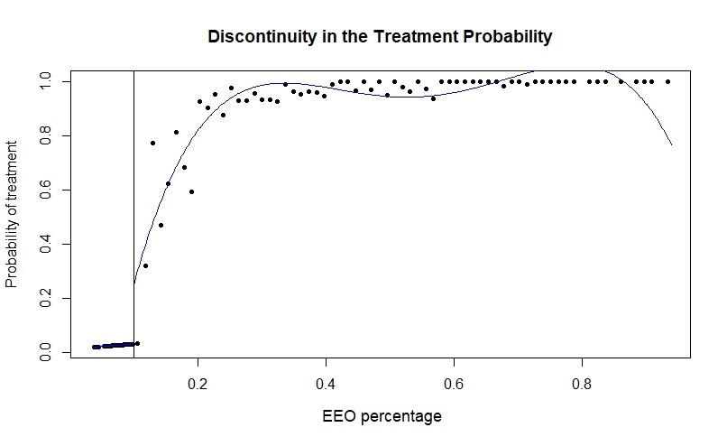
Table 7: Results for 3.5% discontinuity sample with bootstrapped samples of size 50. Standard deviations are in parentheses and the p-value corresponds to a t-test for the difference between the means in the group above and below the threshold.

Appendix D Robustness Checks for Policy Evaluation

D.1 Progress in School

The second outcome variable, progress school, assumes value 1 if the student progresses to the following year without any grade retention and 0 if not: roughly 98% of the students in the sample manage to progress in school in the first two years of secondary education. For the students unable to progress in school, this variable is used as a proxy of negative achievements. Therefore, it is relevant to understand if additional funding was effective in driving students away from negative performance. Figure D.1 depicts the heterogeneous conditional CACEs: the darker the shade of green in the node, the higher the causal effect.

The additional funding has a slightly negative, but statistically insignificant, impact on the chance of progress in school for the overall students in the sample (again, this is in line with what was found by D’Inverno et al. 2021 at the school level). Nevertheless, rather than focusing on the overall average effect, it is more interesting to explore the heterogeneous effects.

The first driver of heterogeneity is the sex of the student. In this case, the funding seems to be effective, even if not significant for the male students, while it is not-effective, and has even a slightly negative effect for the female students. The first driver of heterogeneity is the seniority level of principals: the treatment has an increased effect for students in schools with less senior principals (less than 30 years of experience). In particular, for male students in treated schools with principals with less than 30 years of experience there is an increase of 1.6% in the probability of progressing through school. On the the opposite side, for female students with more senior teachers there is a decrease of 5% in the probability of progressing through school.

Clearly, these characteristics could possibly correlate with unobservables, such as the effectiveness of principals (which may decrease as principals grow older). In any case, this finding opens up new fields for further investigation, in line with the newly established role of machine learning in the economic literature as a “theory-driving/theory-testing” tool (Mullainathan and Spiess 2017).

Figure D.1: Visualization of the heterogeneous Complier Average Causal Effects (CACE) of additional funding on Progress School estimated using the proposed BCF-IV model. The overall sample (discovery plus inference subsamples) size is 4,450. The tree is a summarizing classification tree fit to posterior point estimates of individual treatment effects. The significance level is * for a significance level of 0.1, ** for a significance level of 0.05 and *** for a significance level of 0.01.

D.2 Sampling Variations

This Section tests the robustness of our models to sampling variations. The sampling variations introduced come from the following two sources: (i) a wider bandwidth around the threshold (changing from 3.5% to 3.7%); (ii) an expansion in the number of sampled units (from 50 up to the lowest number of students per school, which is 62). Moreover, an algorithm which detects the heterogeneity in the ITT effects is applied (BCF-ITT). To understand if the balance and the results are robust, we manifest the balance in the averages in the samples of units assigned to the treatment and assigned to the control (Tables 8, 9, 10), the results of the causal effects when we increase the number of units sampled (Figures D.2 and D.3) and the results for the BCF-ITT algorithm (Figures D.4 and D.5).

In all the different samples the school level characteristics remain widely balanced (with the exception of teacher seniority).¹⁶¹⁶ 16 This could be due to the fact that less senior principals select themselves in schools with a lower percentage of disadvantaged students. Primary retention and Sex seem to be slightly unbalanced when we widen the bandwidth, this however holds true just in the case where we sample through bootstrap 50 units (Sex in this case gets back to a good balance).

With respect to the results of the BCF-IV algorithm, when we increase the number of sampled units the main differences between the results for the sample of 50 students for the A-certificate outcome (Figure 3) and the ones for the sample of 62 students (Figure D.2) are the following: (i) the first split is performed on the age of the principal, however this time the chosen split category is being younger or older than 60 years old (in Figure 3 it was 55 years old); (ii) the split on the seniority level of the teacher disappears. With respect to the Progress School outcome (Figure D.1 vs Figure D.3) the main differences are: (i) the first split is performed on the seniority of principals (that was detected as an important variable also in Figure D.1); (ii) the less senior principals seem to boost the effect for students in schools consistently with the results from the analysis on the sample of 50 students; (iii) for the subgroup of students in schools with principals with less than 30 years of experience and without primary retention the additional funding leads to a significant increase of 2.6% in the probability of progressing to the next year of school; and (iv) for the subgroups of (a) students in schools with principals with seniority of 30 years of more, (b) female students in schools with principals with seniority of 30 years of more, (c) retained students in schools with principals with seniority of less than 30 years, the additional funding leads to a significant decrease of 8.1%, 7.4% and 9.4% in the probability of progressing through school, respectively. The results for both trees hint, consistently with the main analysis, at an important role of principal’s age and seniority. Moreover, the significance of the results for the heterogeneous effects in the case of the Progress School outcome hint at the fact that non-significance of the treatment effect is probably due to the smaller number of observations in the nodes in the main analysis.

D.3 ITT Analyses

Figures D.4 and D.5 depict the results obtained from the BCF-ITT. Figure D.4 depicts the results for the ITT for the A-certificate, while Figure D.5 depicts the results for the ITT for the Progress School. The results again are robust with the ones of the main analyses in highlighting the role of principals age and seniority as drivers of the heterogeneity in the effects.

	Above Threshold		Below Threshold		Full Sample		p-value
Retention	0.039	(0.194)	0.035	(0.184)	0.037	(0.189)	0.418
Sex	0.471	(0.499)	0.493	(0.500)	0.482	(0.499)	0.110
Special Needs	0.001	(0.039)	0.000	(0.000)	0.001	(0.027)	0.045
Teacher Age	4.024	(0.269)	4.002	(0.333)	4.023	(0.304)	0.793
Teacher Seniority	3.926	(0.341)	3.867	(0.452)	3.895	(0.404)	0.000
Teacher Training	0.982	(0.025)	0.981	(0.026)	0.982	(0.026)	0.126
Principal Age	5.951	(1.228)	6.002	(1.308)	5.988	(1.271)	0.041
Principal Seniority	5.829	(0.934)	5.777	(1.227)	5.802	(1.097)	0.083
Observations	2790		2542		5332

Table 8: Results for 3.5% discontinuity sample with bootstrapped samples of size 62. Standard deviations are in parentheses and the p-value corresponds to a t-test for the difference between the means in the group above and below the threshold.

	Above Threshold		Below Threshold		Full Sample		p-value
Retention	0.030	(0.170)	0.042	(0.201)	0.036	(0.186)	0.025
Sex	0.497	(0.500)	0.461	(0.499)	0.479	(0.500)	0.015
Special Needs	0.000	(0.021)	0.001	(0.037)	0.001	(0.030)	0.309
Teacher Age	4.022	(0.333)	4.023	(0.260)	4.022	(0.299)	0.955
Teacher Seniority	3.867	(0.452)	3.932	(0.330)	3.899	(0.398)	0.000
Teacher Training	0.982	(0.025)	0.983	(0.026)	0.983	(0.026)	0.805
Principal Age	6.022	(1.308)	6.000	(1.206)	6.011	(1.259)	0.556
Principal Seniority	5.778	(1.228)	5.818	(0.912)	5.798	(1.083)	0.212
Observations	2250		2200		4450

Table 9: Results for 3.7% discontinuity sample with bootstrapped samples of size 50. Standard deviations are in parentheses and the p-value corresponds to a t-test for the difference between the means in the group above and below the threshold.

	Above Threshold		Below Threshold		Full Sample		p-value
Retention	0.029	(0.168)	0.040	(0.196)	0.034	(0.182)	0.026
Sex	0.490	(0.500)	0.464	(0.499)	0.477	(0.500)	0.058
Special Needs	0.000	(0.019)	0.001	(0.038)	0.001	(0.030)	0.174
Teacher Age	4.022	(0.333)	4.023	(0.260)	4.022	(0.299)	0.950
Teacher Seniority	3.867	(0.452)	3.932	(0.330)	3.899	(0.398)	0.000
Teacher Training	0.982	(0.025)	0.983	(0.026)	0.983	(0.026)	0.784
Principal Age	6.022	(1.308)	6.000	(1.206)	6.011	(1.259)	0.512
Principal Seniority	5.778	(1.227)	5.818	(0.912)	5.798	(1.083)	0.165
Observations	2790		2728		5518

Table 10: Results for 3.7% discontinuity sample with bootstrapped samples of size 62 (the smallest school in the sample). Standard deviations are in parentheses and the p-value corresponds to a t-test for the difference between the means in the group above and below the threshold.

Figure D.2: Visualization of the heterogeneous Complier Average Causal Effects (CACE) of additional funding on A-certificate estimated using the proposed BCF-IV model. The overall sample (discovery plus inference subsamples) size is 5,332. The tree is a summarizing classification tree fit to posterior point estimates of individual treatment effects. The significance level is * for a significance level of 0.1, ** for a significance level of 0.05 and *** for a significance level of 0.01.

Figure D.3: Visualization of the heterogeneous Complier Average Causal Effects (CACE) of additional funding on Progress School estimated using the proposed BCF-IV model. The overall sample (discovery plus inference subsamples) size is 5,518. The tree is a summarizing classification tree fit to posterior point estimates of individual treatment effects. The significance level is * for a significance level of 0.1, ** for a significance level of 0.05 and *** for a significance level of 0.01.

Figure D.4: Visualization of the heterogeneous Complier Average Causal Effects (CACE) of additional funding on A-certificate estimated using the proposed BCF-ITT model. The overall sample (discovery plus inference subsamples) size is 5,332. The tree is a summarizing classification tree fit to posterior point estimates of individual treatment effects. The significance level is * for a significance level of 0.1, ** for a significance level of 0.05 and *** for a significance level of 0.01.

Figure D.5: Visualization of the heterogeneous Complier Average Causal Effects (CACE) of additional funding on Progress School estimated using the proposed BCF-ITT model. The overall sample (discovery plus inference subsamples) size is 5,518. The tree is a summarizing classification tree fit to posterior point estimates of individual treatment effects. The significance level is * for a significance level of 0.1, ** for a significance level of 0.05 and *** for a significance level of 0.01.