Limited-control metrology approaching the Heisenberg limit without entanglement preparation

Benedikt Tratzmiller Affiliation: Institut für Theoretische Physik and IQST, Albert-Einstein-Allee 11, Universität Ulm, D-89081 Ulm, Germany Qiong Chen Affiliation: Institut für Theoretische Physik and IQST, Albert-Einstein-Allee 11, Universität Ulm, D-89081 Ulm, Germany Affiliation: College of Physics and Electronics, Hunan Normal University, Changsha 410081, China Ilai Schwartz Affiliation: Institut für Theoretische Physik and IQST, Albert-Einstein-Allee 11, Universität Ulm, D-89081 Ulm, Germany Affiliation: NVision Imaging Technologies GmbH, Albert-Einstein-Allee 11, Universität Ulm, D-89081 Ulm, Germany Susana F. Huelga Affiliation: Institut für Theoretische Physik and IQST, Albert-Einstein-Allee 11, Universität Ulm, D-89081 Ulm, Germany Martin B. Plenio Affiliation: Institut für Theoretische Physik and IQST, Albert-Einstein-Allee 11, Universität Ulm, D-89081 Ulm, Germany

August 11, 2026

Abstract

Current metrological bounds typically assume full control over all particles that are involved in the protocol. Relaxing this assumption we study metrological performance when only limited control is available. As an example, we measure a static magnetic field when a fully controlled quantum sensor is supplemented by particles over which only global control is possible. We show that even for a noisy quantum sensor, a protocol that maps the magnetic field to a precession frequency can achieve transient super-Heisenberg scaling in measurement time and Heisenberg scaling in the particle number. This leads to an estimation uncertainty that approaches that achievable under full control to within a factor independent of the particle number for a given total time. Applications to hybrid sensing devices and the crucial role of the quantum character of the sensor are discussed.

I Introduction

The use of quantum resources in sensing and metrology has a longstanding history which originated with the use of single-mode squeezed states Caves 1981 and multi-particle spin-squeezing Wineland et al. 1992; Wineland et al. 1994, i.e., entanglement, to enhance precision in interferometry and atomic spectroscopy.

The goal of quantum metrology is the optimisation of the scaling of metrological precision with the available physical resources Giovannetti et al. 2004; Braun et al. 2018. Notably, in a noiseless setting, independent preparation and measurement of $M$ particles in parallel results in a $1/\sqrt{M}$ scaling of the uncertainty, the so called standard quantum limit (SQL), while the collective preparation of the particles in an entangled state leads to a $1/M$ -scaling, commonly referred to as Heisenberg scaling (HS) Wineland et al. 1992; Wineland et al. 1994 (see Hyllus et al. 2012; Tóth and Petz 2013 for more general upper bounds obtained via the quantum Fisher information). The use of entangled states is necessary to achieve the optimal precision and exact HS but sequences of probe states with an asymptotically vanishing amount of entanglement can reach a scaling arbitrarily close to the Heisenberg limit (HL) Augusiak et al. 2016. Environmental noise is known to have a non-trivial impact on metrology Huelga et al. 1997 and a meaningful comparison of different schemes needs to specify carefully the conditions under which the metrological protocol is carried out, such as the number of particles or the total amount of time available Huelga et al. 1997; Escher et al. 2011. A wide variety of setting has been analysed Huelga et al. 1997; Escher et al. 2011; Demkowicz-Dobrzański et al. 2012; Haase et al. 2018 and noise models have been found to result in metrological scaling intermediate between SQL and the HL Chin et al. 2012; Matsuzaki et al. 2011; Macieszczak 2015; Smirne et al. 2016; Haase et al. 2018. However, these results depend on access to perfect and arbitrarily fast control and feedback operations Sekatski et al. 2017; Demkowicz-Dobrzański and Maccone 2014.

In practice, however, only limited control is possible over experimental resources and the asymptotic regime of large numbers of fully controlled particles is not accessible. What can be achieved in metrology for systems where, for example, particles cannot be addressed individually, multi-particle quantum gates are not available or the rate of measurements, feedback and the number of accessible particles is limited?

In order to initiate investigations of this type in a concrete setting, we allow ourselves to be motivated by the recently developed concept of quantum-hybrid sensors Cai et al. 2014; Wrachtrup and Finkler 2014. These are devices that integrate at least two components, one being a fully controlled quantum sensor and another, typically an assembly of quantum particles, mutually interacting or not, that are coupled to the quantum sensor but over which there is no individual control. This second component acts as a transducer of a signal to a form that is then detected by the quantum sensor. An example is a device composed of a piezo-magnetic material deposited on a diamond surface that translates a force into a stray magnetic field which is then detected by a shallowly implanted nitrogen-vacancy (NV) center in diamondGruber et al. 1997; Müller et al. 2014; Wu et al. 2016. Another possibility, motivated by recently realised nanoscale NMR measurements Schmitt et al. 2017; Boss et al. 2017; Glenn et al. 2018, consists of an ensemble of $M$ nuclear spins and an NV center. Here an applied magnetic field can be measured as it induces a nuclear Larmor precession which can be monitored by an NV center. Similarly, atoms in microfabricated vapour cells Shah et al. 2007 could allow for observation of their Larmor precession by an NV center rather than a classical laser field. We assume that the quantum sensor is subject to noise, and cannot exert individual control over the noise-free auxiliary spins.

While we are motivated by concrete settings, our analysis yields more compact expressions, without affecting the scaling properties, by assuming that all involved spins have the same magnetic moment. Furthermore, all the following considerations will neglect direct interactions between the auxiliary spins.

By means of analyzing the scaling of the Fisher information with respect to particle number $M$ and measurement time $T$ we will show that, despite the limitations of partial control, it is possible to get close to the Heisenberg limit, we will discuss the origin of this scaling and compare our scheme to a single quantum sensor without auxiliary spins.

Figure 1: The proposed measurement scheme uses a control sequence on the sensor spin (blue) to weakly measure the auxiliary spins (black) without the need of further control after initialisation in either the pure state

\ket{+++...}

as shown here or the completely mixed state. The weak measurement is realised by initialising a sensor spin (blue) into

\ket{0}

, applying

\pi/2

-pulses and a dynamical decoupling (DD) sequence to weakly entangle the sensor spin with the auxiliary spins and finally measuring the sensor spin, applying an effective CPTP map onto the auxiliary spins. In between these measurements that are synchronised with an external local oscillator, the auxiliary spins acquire a phase

\phi\propto{\mu_{n}}B

, leading to a total phase

n\phi

after

n

cycles.

II Approaching the Heisenberg limit without entanglement preparation

Before stating the main results, we briefly recapitulate the achievable uncertainties under unconstrained metrology to make it available for later comparison with our schemes.

II.1 The ideal case of full quantum control

Consider a quantum sensor and $M$ auxiliary spins, all with the same magnetic moment ${\mu_{n}}$ , over which we can exert arbitrary and fast control. Then the optimal uncertainty for the estimation of the magnetic field in a time $T$ in the absence of noise is obtained via Ramsey spectroscopy using the $M+1$ accessible particles prepared in a highly entangled state of the form $(|0\ldots 0\rangle+|1\ldots 1\rangle)/\sqrt{2}$ and is given by Huelga et al. 1997

\Delta B=\frac{\hbar}{{\mu_{n}}(M+1)T}.

(1)

We observe a linear decrease in the uncertainty, i.e. HS, both in the total measurement time $T$ and the number of spins $M$ .

II.2 The case of limited control setting

We consider a perfectly controlled quantum sensor supplemented by $M$ auxiliary spins all having the same magnetic moment. These $M$ auxiliary spins can be controlled by a global field and interact weakly with the quantum sensor, i.e. the product of sensor-auxiliary spin interaction strength and interaction time is much smaller than unity. For simplicity we assume that each auxiliary particle is interacting with the same strength and phase with the quantum sensor, however the basic findings remain the same in the more general case.

We measure a static external magnetic field $B$ with this hybrid sensor and determine the achievable uncertainty $\Delta B$ . To this end we initialise the auxiliary spins in a fully polarised state FN1 and then subject them to a $\pi/2$ -pulse. We determine the resulting rate of precession of these $M$ spins by periodically measuring the time-dependent magnetic field generated by the precessing spins in regular time intervals using the quantum sensor and a dynamical decoupling (DD) sequence to weakly entangle it with the auxiliary spins. This allows for comparison of the precession frequency to that of a local oscillator Schmitt et al. 2017; Boss et al. 2017 as sketched in figure 1. This DD sequence does not only cancel static noise on the sensor spin, but also allows to accumulate signal over several auxiliary spin Larmor periods by creating an effective $\sigma_{z}\otimes\sigma_{x}$ interaction. In order to see this, we start with a Hamiltonian of the form

	$\displaystyle H=\frac{\Omega(t)}{2}\sigma_{x}$	$\displaystyle+\sum_{m=1}^{M}\frac{\omega_{L}}{2}\sigma_{z}^{(m)}$		(2)
		$\displaystyle+A_{\perp}^{(m)}\sigma_{z}\otimes\left(\sigma_{x}^{(m)}\cos({\phi_{0m}})+\sigma_{y}^{(m)}\sin({\phi_{0m}})\right)$

that describes a NV center coupled to $M$ nuclear spins in the interaction picture where $\Omega(t)$ is the Rabi frequency with $\Omega(t)=0$ during the free evolution, $\omega_{L}$ is the nuclear Larmor frequency, $A_{\perp}^{(m)}$ is the perpendicular coupling of the nuclear spins and $\phi_{0m}$ the corresponding phase. The operators $\sigma_{i}$ act on the electron spin (NV center), $\sigma_{i}^{(m)}$ act on the mth nuclear spin.

When we fulfil $\tau=\pi/\omega_{L}$ in the DD (e.g. XY-8) sequence, the sequence produces a modulation function that modulates the NV $\sigma_{z}$ operator to $\sigma_{z}f(t)$ where

f(t)=\frac{4}{\pi}\cos(\omega_{L}t)+\mathrm{rot.}

(3)

and rot. denotes terms that vanish after the rotating-wave approximation in a frame rotating with the nuclear Larmor frequencies. Using

\cos^{2}(\omega_{L}t)=\frac{1}{2}\left(1+\cos(2\omega_{L}t)\right),

(4)

we obtain the effective interaction Hamiltonian

H_{\mathrm{eff}}=\sum\limits_{m}\frac{2A_{\perp}^{(m)}}{\pi}\sigma_{z}\otimes\left(\sigma_{x}^{(m)}\cos({\phi_{0m}})+\sigma_{y}^{(m)}\sin({\phi_{0m}})\right)

(5)

that will be the starting point for the following discussion.

We use ${k_{0}}={\mu_{n}}B_{s}/\hbar$ where $B_{s}$ is the field generated by one of the $M$ auxiliary spins at the position of the NV center

II.3 Transient super-Heisenberg scaling in measurement time

In a first step we analyse the Fisher information scaling with the measurement time. For this purpose we derive the probability $p_{n}$ of finding the internal state of a spin- $1/2$ quantum sensor in the spin-down state in the n-th measurement in leading order assuming the length $T_{s}$ of each instance of a magnetic field measurement is short and if we apply these measurements every $\tau_{m}$ .

We simplify to the case that all couplings $A_{\perp}^{(m)}=k$ and all phases $\phi_{m}$ are equal, see the appendix for a more general discussion. Here $k_{0}={\mu_{n}}B_{s}/\hbar$ where $B_{s}$ is the field generated by one of the $M$ auxiliary spins at the position of the NV center. In the described protocol the auxiliary spins gain a phase $\phi=\delta\tau_{m}$ in each step, where $\delta=2\pi(\nu-\nu_{loc})$ is the difference of precession frequency $\nu$ and local oscillator frequency $\nu_{loc}$ . For a nuclear spin with an already accumulated phase from $n$ cycles equalling $n\phi$ the readout probability is calculated for the NV measurement in basis $Y$ , i.e. the eigenbasis of the Pauli $,\sigma_{y}$ operator, and NV preparation in $\ket{+}$ .

$\displaystyle p_{n}$	$\displaystyle-\frac{1}{2}=\mathrm{Tr}\left[\hat{O}_{\mathrm{measurement}}U\rho_{n}U^{\dagger}\right]$
	$\displaystyle=\mathrm{Tr}\left[\left(\frac{\sigma_{y}}{2}\otimes\mathbbm{1}^{\otimes M}\right)U\right.$
	$\displaystyle\left.\left(\frac{\mathbbm{1}+\sigma_{x}}{2}\otimes\left(\frac{\mathbbm{1}+\cos(\phi n)\sigma_{x}+\sin(\phi n)\sigma_{y}}{2}\right)\right)^{\otimes M}U^{\dagger}\right]$
	$\displaystyle=\frac{i}{4}\left[\left(\cos\frac{4k_{0}T_{s}}{\pi}-i\sin\frac{4k_{0}T_{s}}{\pi}\cos(\phi n)\right)^{M}\right.$
	$\displaystyle\left.-\left(\cos\frac{4k_{0}T_{s}}{\pi}+i\sin\frac{4k_{0}T_{s}}{\pi}\cos(\phi n)\right)^{M}\right].$	(6)

For $Mk_{0}T_{s}\ll 1$ we can approximate

		$\displaystyle\left(\cos\frac{4k_{0}T_{s}}{\pi}\pm i\sin\frac{4k_{0}T_{s}}{\pi}\cos(\phi n)\right)^{M}$
		$\displaystyle\cong\exp\left(\pm iM\sin\frac{4k_{0}T_{s}}{\pi}\cos(\phi n)\right)$		(7)

to derive the signal

p_{n}=\cos^{2}\left(\frac{2M{k_{0}}T_{s}}{\pi}\cos\left(\phi n\right)-\frac{\pi}{4}\right).

(8)

Imperfect polarisation $P$ of the auxiliary spins can be incorporated via $k_{0}=\mu_{n}PB_{s}/\hbar$ .

By eq. (8) we estimate the frequency $2\pi\nu={\mu_{n}}B/\hbar$ and hence the magnitude of the magnetic field $B$ . For $N$ measurements, the achievable uncertainty in the estimate of $\nu$ is obtained via the classical Fisher information

{I_{N}=\sum_{n=1}^{N}\frac{1}{p_{n}(1-p_{n})}\left(\frac{\partial p_{n}}{\partial\phi}\right)^{2}\left(\frac{\partial\phi}{\partial\delta}\right)^{2}.}

(9)

We can describe decoherence processes in terms of a decay rate $\gamma=\gamma_{2}+\gamma_{b}$ (see appendix), where $\gamma_{2}$ refers to $T_{2}$ processes on the nuclear spins and $\gamma_{b}$ refers to measurement backaction from the quantum sensor. Then the effective coupling after $n$ measurements is $k_{n}=k_{0}e^{-\gamma n}$ and we find

\displaystyle I_{N}(\gamma)=\sum_{n=1}^{N}\left(\frac{4\tau_{m}Mk_{n}T_{s}n}{\pi}\right)^{2}\sin^{2}\phi n.

(10)

Under the assumptions $max[\gamma,\frac{1}{N}]\ll 2\pi\phi$ and $Mk_{0}T_{s}\ll 1$ , i.e. when we sample at least one full oscillation of the signal of frequency $\delta$ , eq. (10) is well approximated by

	$\displaystyle I_{N}(\gamma)$	$\displaystyle\cong$	$\displaystyle\frac{16M^{2}\tau_{m}^{2}k_{0}^{2}T_{s}^{2}}{\pi^{2}}\sum_{n=1}^{N}\frac{n^{2}}{2}e^{-2\gamma n}\left(1-\cos 2\phi n\right)$		(11)
		$\displaystyle\cong$	$\displaystyle\frac{2M^{2}\tau_{m}^{2}k_{0}^{2}T_{s}^{2}}{\pi^{2}}\frac{1-e^{-2\gamma N}(1+2\gamma N(1+\gamma N))}{\gamma^{3}}.$		(11)

For $\gamma N\ll 1$ (for $\gamma N<0.6$ errors are smaller than 3%)

\displaystyle I_{N}(\gamma)\cong\frac{2M^{2}\tau_{m}^{2}k_{0}^{2}T_{s}^{2}}{\pi^{2}}(\frac{4N^{3}}{3}-2\gamma N^{4}+\frac{6\gamma^{2}N^{5}}{5})

(12)

and hence

\displaystyle\Delta B

\displaystyle\leq

\displaystyle\sqrt{\frac{3\pi^{2}\hbar^{2}}{8{\mu_{n}}^{2}M^{2}\tau_{m}^{2}k_{0}^{2}T_{s}^{2}}\frac{1}{N^{3}}}.

(13)

As a result, for small $\gamma N$ our limited control procedure exhibits a scaling in the number of measurements $N$ or, equivalently, the total measurement time $T=N\tau_{m}$ that exceeds the standard HS of eq. (1) while the scaling in the number of particles $M$ achieves the HL. Note that unlike the case of interaction-based quantum metrology Boixo et al. 2007 this super-Heisenberg scaling is not due to interactions between the auxiliary spins. Intuitively the scaling can be understood to emerge due to the fact that, without noise, the last measurement of the measurement record alone would already give quadratic Fisher information scaling, and the linear number of intermediate measurements leads to a cubic scaling in total.

II.4 Asymptotic SQL scaling in measurement time

However, the super-Heisenberg scaling identified in the previous subsection has to be transient and cannot persist for arbitrarily long times as this would be in violation of the fundamental limit of sensitivity that is imposed by the full control scheme in the absence of any noise.

For $\gamma_{2}=0$ , the remaining contribution to the decay rate $\gamma$ is due to the measurement backaction of the quantum sensor on the auxiliary spins which is negligible only for $\gamma N\ll 1$ . Our measurement scheme then yields (see appendix for a derivation)

\gamma_{b}=\frac{4k_{0}^{2}T_{s}^{2}}{\pi^{2}}.

(14)

Due to the measurement backaction, the signal weakens with increasing number of measurements $N$ and the rate of increase of the Fisher information slows. When determining the scaling in this regime, a note of caution is in order as the calculation of the measurement backaction in eq. (11) determines the Fisher information of the averaged density matrix of the auxiliary spins. However, as we have access to and use all the intermediate measurements, the correct Fisher information of the protocol is obtained by weighted averaging over measurement trajectories. For $\gamma N\gg 1$ this results in a scaling linear in $N$ (see also Pfender et al. 2019; Clark et al. 2019; Cohen et al. 2019), as indicated analytically in the appendix and numerically in figure 2. For $M=100$ nuclei in an initial product state (red data) the transient super-Heisenberg $I_{N}\propto N^{3}\propto T^{3}$ scaling evolves into the shot noise scaling (SQL) of $I_{N}\propto N\propto T$ (blue asymptote) while eq. (11) was calculated with the average density matrix and therefore would yield a constant. Remarkably, this linear scaling is independent of the initial state and we can achieve the same scaling using a completely mixed initial state (orange triangles) Foo. In the limit of small interaction strength $k_{0}T_{s}$ and decay, the asymptotic ( $\gamma N\gg 1$ ) value of the Fisher information can be estimated to be

I_{N}=\frac{\sin^{4}(4k_{0}T_{s}/\pi)}{16\left(\gamma_{b}+\gamma_{2}\right)^{3}}\frac{M^{2}}{2}\tau_{m}^{2}N

(15)

Refer to caption — Figure 2: Upper graph: Numerical Fisher information scaling (red: initial product state/ orange: initial mixed state), the analytical approximation for small $N$ eq. (11) (red line, invalid for large N due to the average density matrix calculation being invalid for $\gamma N>1$ ) and the asymptotic ( $\gamma N\gg 1$ ) behaviour (blue) for $\phi=0.7$ and M=100 nuclear spins, each coupled with $k_{0}T_{s}=0.01$ to the NV center. The HL (black) for $M+1$ spins is shown for comparison. The results are averaged over 96 (32 for mixed state) runs with $N=2^{26}$ measurements each. Lower graph: Same data (red) and results for $k_{0}T_{s}=0.05$ in green. The Fisher information is initially larger but dominated by backaction earlier, resulting in a smaller prefactor for the asymptotic regime. In both graphs and all other simulations the achievable Fisher information approaches the HL to within a factor $\lesssim 20$ . This Fisher minimal distance is independent of the interaction strength $k_{0}T_{s}$ and the number of nuclei $M$ , see appendix.

II.5 Heisenberg scaling in particle number and relation to the Heisenberg limit

While the quadratic scaling with the number of nuclei $M$ is obvious for $\gamma N\ll 1$ , it also persists for $\gamma N\gg 1$ as confirmed in equation (15) and in Fig. 3 (see Fig. 4 and the related discussion for details). In the full control scenario such a quadratic scaling can be traced back to the preparation of an macroscopically entangled resource state of the form $(|0...0\rangle+|1...1\rangle)/\sqrt{2}$ including the quantum sensor and the auxiliary spins which contain one ebit of entanglement Vedral and Plenio 1998; Plenio 2005. This entanglement is destroyed with the final measurement and represents the resource that is required to achieve HS. This is in sharp contrast with our scenario, which starts from an initial product state. Here the quadratic scaling arises because the auxiliary spins are interrogated by a quantum sensor which results in a readout operator that is not particle local, i.e. cannot be represented by a product of single particle operators as would be the case when using a classical readout device. Indeed, every measurement applies a CPTP (completely positive and trace-preserving) map to the auxiliary spins that is represented by the Kraus operators (see also Pfender et al. 2019 for the case $M=1$ and our appendix)

U_{\pm}=\bra{\pm_{y}}U\ket{+}=\frac{e^{-i\frac{2k_{0}T_{s}}{\pi}\sum\sigma_{x}^{(m)}}\mp ie^{i\frac{2k_{0}T_{s}}{\pi}\sum\sigma_{x}^{(m)}}}{2}

(16)

Crucially, this operator is diagonal in a basis different than the eigenbasis of the free evolution operator - the latter being a tensor product of unitary evolutions on every auxiliary spin. If the same held true for the readout operator, it is trivial to see that every spin would be measured independently and therefor SQL scaling would apply. The readout operator here, however, combines all particle states in a nontrivial, nonlocal, manner. This is similar to the metrological advantage obtained for indistinguishable particles Braun et al. 2018 (section III). In our work, this advantage is achieved by the sensor spin that, unlike a classical sensor, allows to apply the same, particle non-local, CPTP map in every measurement. We would like to stress that the entanglement build-up due to the backaction via a non-local measurement operator does not contribute to the quadratic scaling with the number of auxiliary spins, nor does it support the transient $N^{3}$ super-Heisenberg scaling.

In the limit of large nuclear coherence times $0\approx\gamma_{2}\ll\gamma_{b}$ the Fisher information approaches the HL achievable under full control for $N_{opt}\approx\left({2k_{0}T_{s}}/{\pi}\right)^{-2}=1/\gamma_{b}$ measurements after which the $N^{3}$ -scaling turns into a scaling $\propto N$ . Note that the fundamental Heisenberg limit is not violated as with decreasing interaction $k_{0}T_{s}$ both the backaction and the information gain per measurement decrease at the same rate thus compensating each other. Remarkably, at this point the ratio of ultimate sensitivity under global control and the limited control scheme used here only depends on the interaction strength and therefore can be tuned to approach the HL for $N_{opt}$ measurements to within a Fisher minimal distance of a factor independent of $T$ , see figure 2. Furthermore it is natural to assume that this holds independently of $M$ as the Fisher information of both the HL and the asymptote for $\gamma N\gg 1$ exhibit the same quadratic in $M$ scaling. This was confirmed numerically (see appendix for confirmation).

III Discussion

Metrology assisted by environmental spins have been considered before, see e.g. Goldstein et al. 2011; Cappellaro et al. 2012. There, however, the emphasis was placed on spins that are strongly interacting with the quantum sensor and the measurement protocol creates a joint entangled state of the quantum sensor and the auxiliary spins which then evolves for some time followed by an inversion of the entangling operation and the subsequent measurement of the state of the quantum sensor. In this approach the HS is achieved in the number of strongly coupled auxiliary spins while we assume no such spins in our set-up. Furthermore, this protocol suffers from the drawback that it is fundamentally limited by the coherence time of the quantum sensor and hence does not take full advantage of the long coherence time of the auxiliary spins. In contrast, the measurements in our protocol can be made shorter than the coherence time without adversely affecting the achievable sensitivity.

Besides the theoretical interest in the novel scaling regimes, we stress that the proposed scheme employing auxiliary spins under limited control provides enhanced sensitivity as compared to the quantum sensor alone. This advantage is the result of two processes. First, the transduction of the static magnetic field to a time-dependent Larmor precession which is then detected by the quantum sensor facilitates the use of dynamical decoupling schemes to filter out noise without adversely affecting the signal. Secondly, as each auxiliary spin contributes to the signal, the overall signal strength scales with the number of spins and hence leads to a considerable signal enhancement. Remarkably, magnetometry schemes such as atoms in gas cells which are probed independently by a classical field lead to a $M^{-1}$ scaling of the variance with the particle number $M$ . In sharp contrast, it is the transduction of the signal to a quantum sensors, e.g. an NV center, which results in a particle non-local measurement which causes the $M^{-2}$ Heisenberg scaling. This suggests a practical route for enhancing the measurement capacity of gas cell magnetometers. Furthermore, for an NV center as quantum sensor, even when considering nuclei with their small magnetic moment as auxiliary spins, we may obtain an increased sensitivity. To this end, let us consider the $|m=0\rangle\leftrightarrow|m=+1\rangle$ transition of an NV center in an external magnetic field $B$ and assume that the NV center is dominated by pure dephasing which results in a coherence time $T_{2}^{(NV)}$ . For perfect readout efficiency, the optimal interrogation scheme yields

{\Delta B=\sqrt{\frac{2e\hbar^{2}}{\mu_{e}^{2}T_{2}^{(NV)}T}}=\sqrt{\frac{4e\hbar^{2}}{\mu_{e}^{2}N{T_{2}^{(NV)}}^{2}}}}

(17)

Huelga et al. 1997 where $N=2T/T_{2}^{(NV)}$ . The maximum of equation (15) that takes the form $\gamma_{b}^{2}/(\gamma_{b}+\gamma_{2})^{3}$ is obtained by choosing $\gamma_{b}=2\gamma_{2}$ . This allows to compare with our indirect measurement scheme using $M$ hydrogen nuclear spins and assuming $\left(\frac{\mu_{e}}{{\mu_{n}}}\right)^{2}\frac{T_{2}^{(NV)}}{T_{2}^{n}}\approx 10^{3}$ we find that for

{M>\sqrt{\frac{27}{4e}\frac{\mu_{e}^{2}T_{2}^{(NV)}}{\mu_{n}^{2}T_{2}^{(n)}}}\approx 50}

(18)

the auxiliary spin assisted sensor outperforms the bare NV center. Nuclear spins couple more weakly to both noise and signal due to smaller gyromagetic ratio resulting in typically larger coherence times $\frac{\mu_{e}}{{\mu_{n}}}\approx\frac{T_{2}^{n}}{T_{2}^{(NV)}}$ , so similar results apply for other systems. While our protocol makes use of a far smaller magnetic moment compared to even a single electron spin $M\mu_{n}\ll\mu_{e}$ , this is compensated by the longer coherence time and the possibility to measure during the signal accumulation.

Furthermore the obtained expression also highlights the advantage of the $M^{-2}$ Heisenberg scaling over the SQL that individual measurements on the nuclear spins give, providing higher Fisher Information for $M>27/4e\approx 2.5$ .

Finally, we note that our analysis also covers the case $M=1$ corresponding to the detection of the Larmor frequency of a single nuclear spin via an NV center. Super-Heisenberg scaling applies for as long as the measurement backaction is weak. This applies for distant nuclear spins or for measurements that are designed to be weak, i.e. not obtaining a full bit of information in each single measurement.

Conclusions – We have examined metrology in a realistic setting of limited control and found transient super-Heisenberg scaling in the total measurement time and a metrological precision approaching that of the same number of particles under full experimental control. This is despite the absence of initial entanglement in the system. In fact, in this scheme entanglement emerges only with increasing number of measurements and adversely affects the metrological scaling. Furthermore, the proposed set-up, which employs auxiliary spin under limited control, also represents an hybrid sensor that may outperform a bare quantum sensor thus providing new design principles for quantum sensors.

Acknowledgements – The authors thank Liam McGuinness and Jan F. Haase for discussions and comments on the manuscript. This work was supported by the ERC Synergy Grant BioQ, the EU projects AsteriQs, HYPERDIAMOND, the BMBF projects NanoSpin and DiaPol, the DFG CRC 1279 and the DFG project 414061038. The authors acknowledge support by the state of Baden-Württemberg through bwHPC and the German Research Foundation (DFG) through grant no INST 40/467-1 FUGG (JUSTUS cluster). The first results of this work have been presented at the Workshop On Quantum Metrology, 22nd - 23rd June 2017 in Ulm, Germany.

References

Caves (1981) C. M. Caves. Quantum-mechanical noise in an interferometer. Physical Review D, 23(8):1693, 1981.
Wineland et al. (1992) D. J. Wineland, J. J. Bollinger, W. M. Itano, F. Moore, and D. Heinzen. Spin squeezing and reduced quantum noise in spectroscopy. Physical Review A, 46(11):R6797, 1992.
Wineland et al. (1994) D. J. Wineland, J. J. Bollinger, W. M. Itano, and D. Heinzen. Squeezed atomic states and projection noise in spectroscopy. Physical Review A, 50(1):67, 1994.
Giovannetti et al. (2004) V. Giovannetti, S. Lloyd, and L. Maccone. Quantum-enhanced measurements: beating the standard quantum limit. Science, 306(5700):1330–1336, 2004.
Braun et al. (2018) D. Braun, G. Adesso, F. Benatti, R. Floreanini, U. Marzolino, M. W. Mitchell, and S. Pirandola. Quantum-enhanced measurements without entanglement. Reviews of Modern Physics, 90(3):035006, 2018.
Hyllus et al. (2012) P. Hyllus, W. Laskowski, R. Krischek, C. Schwemmer, W. Wieczorek, H. Weinfurter, L. Pezzé, and A. Smerzi. Fisher information and multiparticle entanglement. Physical Review A, 85(2):022321, 2012.
Tóth and Petz (2013) G. Tóth and D. Petz. Extremal properties of the variance and the quantum fisher information. Physical Review A, 87(3):032324, 2013.
Augusiak et al. (2016) R. Augusiak, J. Kołodyński, A. Streltsov, M. N. Bera, A. Acin, and M. Lewenstein. Asymptotic role of entanglement in quantum metrology. Physical Review A, 94(1):012339, 2016.
Huelga et al. (1997) S. F. Huelga, C. Macchiavello, T. Pellizzari, A. K. Ekert, M. B. Plenio, and J. I. Cirac. Improvement of frequency standards with quantum entanglement. Physical Review Letters, 79(20):3865, 1997.
Escher et al. (2011) B. M. Escher, R. L. de Matos Filho, and L. Davidovich. General framework for estimating the ultimate precision limit in noisy quantum-enhanced metrology. Nature Physics, 7(5):406, 2011.
Demkowicz-Dobrzański et al. (2012) R. Demkowicz-Dobrzański, J. Kołodyński, and M. Guţă. The elusive heisenberg limit in quantum-enhanced metrology. Nature Communications, 3:1063, 2012.
Haase et al. (2018) J. F. Haase, A. Smirne, J. Kołodyński, R. Demkowicz-Dobrzański, and S. F. Huelga. Fundamental limits to frequency estimation: a comprehensive microscopic perspective. New Journal of Physics, 20(5):053009, 2018.
Chin et al. (2012) A. W. Chin, S. F. Huelga, and M. B. Plenio. Quantum metrology in non-markovian environments. Physical Review Letters, 109(23):233601, 2012.
Matsuzaki et al. (2011) Y. Matsuzaki, S. C. Benjamin, and J. Fitzsimons. Magnetic field sensing beyond the standard quantum limit under the effect of decoherence. Physical Review A, 84(1):012103, 2011.
Macieszczak (2015) K. Macieszczak. Zeno limit in frequency estimation with non-markovian environments. Physical Review A, 92(1):010102, 2015.
Smirne et al. (2016) A. Smirne, J. Kołodyński, S. F. Huelga, and R. Demkowicz-Dobrzański. Ultimate precision limits for noisy frequency estimation. Physical Review Letters, 116(12):120801, 2016.
Sekatski et al. (2017) P. Sekatski, M. Skotiniotis, J. Kołodyński, and W. Dür. Quantum metrology with full and fast quantum control. Quantum, 1:27, 2017.
Demkowicz-Dobrzański and Maccone (2014) R. Demkowicz-Dobrzański and L. Maccone. Using entanglement against noise in quantum metrology. Physical Review Letters, 113(25):250801, 2014.
Cai et al. (2014) J. Cai, F. Jelezko, and M. B. Plenio. Hybrid sensors based on colour centres in diamond and piezoactive layers. Nature Communications, 5:4065, 2014.
Wrachtrup and Finkler (2014) J. Wrachtrup and A. Finkler. Applied physics: Hybrid sensors ring the changes. Nature, 512(7515):380, 2014.
Gruber et al. (1997) A. Gruber, A. Dräbenstedt, C. Tietz, L. Fleury, J. Wrachtrup, and C. Von Borczyskowski. Scanning confocal optical microscopy and magnetic resonance on single defect centers. Science, 276(5321):2012–2014, 1997.
Müller et al. (2014) C. Müller, X. Kong, J.-M. Cai, K. Melentijević, A. Stacey, M. Markham, D. Twitchen, J. Isoya, S. Pezzagna, J. Meijer, et al. Nuclear magnetic resonance spectroscopy with single spin sensitivity. Nature Communications, 5:4703, 2014.
Wu et al. (2016) Y. Wu, F. Jelezko, M. B. Plenio, and T. Weil. Diamond quantum devices in biology. Angewandte Chemie International Edition, 55(23):6586–6598, 2016.
Schmitt et al. (2017) S. Schmitt, T. Gefen, F. M. Stürner, T. Unden, G. Wolff, C. Müller, J. Scheuer, B. Naydenov, M. Markham, S. Pezzagna, et al. Submillihertz magnetic spectroscopy performed with a nanoscale quantum sensor. Science, 356(6340):832–837, 2017.
Boss et al. (2017) J. M. Boss, K. S. Cujia, J. Zopes, and C. L. Degen. Quantum sensing with arbitrary frequency resolution. Science, 356(6340):837–840, 2017.
Glenn et al. (2018) D. R. Glenn, D. B. Bucher, J. Lee, M. D. Lukin, H. Park, and R. L. Walsworth. High-resolution magnetic resonance spectroscopy using a solid-state spin sensor. Nature, 555(7696):351, 2018.
Shah et al. (2007) V. Shah, S. Knappe, P. D. D. Schwindt, and J. Kitching. Subpicotesla atomic magnetometry with a microfabricated vapour cell. Nature Photonics, 1:649 – 652, 2007.
(28) Our considerations are easily extended to the case of an arbitrary polarisation as the signal and hence the sensitivity is directly proportional to the polarisation level.
Boixo et al. (2007) S. Boixo, S. T. Flammia, C. M. Caves, and J. M. Geremia. Generalized limits for single-parameter quantum estimation. Physical Review Letters, 98(9):090401, 2007.
Pfender et al. (2019) M. Pfender, P. Wang, H. Sumiya, S. Onoda, W. Yang, D. B. R. Dasari, P. Neumann, X.-Y. Pan, J. Isoya, R.-B. Liu, et al. High-resolution spectroscopy of single nuclear spins via sequential weak measurements. Nature Communications, 10(1):594, 2019.
Clark et al. (2019) L. A. Clark, A. Stokes, and A. Beige. Quantum jump metrology. Physical Review A, 99(2):022102, 2019.
Cohen et al. (2019) D. Cohen, T. Gefen, L. Ortiz, and A. Retzker. Achieving the ultimate precision limit in quantum nmr spectroscopy. arXiv:1912.09062, 2019.
(33) See also Górecka et al. 2018 for the related observation that for metrology in non-markovian environments the zeno-scaling can be achieved with a mixed initial state.
Vedral and Plenio (1998) V. Vedral and M. B. Plenio. Entanglement measures and purification procedures. Physical Review A, 57(3):1619, 1998.
Plenio (2005) M. B. Plenio. Logarithmic negativity: a full entanglement monotone that is not convex. Physical Review Letters, 95(9):090503, 2005.
Goldstein et al. (2011) G. Goldstein, P. Cappellaro, J. R. Maze, J. S. Hodges, L. Jiang, A. S. Sørensen, and M. D. Lukin. Environment-assisted precision measurement. Physical Review Letters, 106(14):140502, 2011.
Cappellaro et al. (2012) P. Cappellaro, G. Goldstein, J. Hodges, L. Jiang, J. Maze, A. Sørensen, and M. D. Lukin. Environment-assisted metrology with spin qubits. Physical Review A, 85(3):032336, 2012.
Górecka et al. (2018) A. Górecka, F. A. Pollock, P. Liuzzo-Scorpo, R. Nichols, G. Adesso, and K. Modi. Noisy frequency estimation with noisy probes. New Journal of Physics, 20:083008, 2018.

Appendix: Limited-control metrology approaching the Heisenberg limit without entanglement preparation

Appendix A Derivation of the signal for few measurements

This section presents a more general calculation of equations (6-8) of the main text. For a nuclear spin (initial state described by polarisation P) with an already accumulated phase from $n$ cycles $\phi_{1m}=\delta\tau_{m}n+\phi_{0}$ the readout probability is (NV measurement in basis $Xc_{\alpha}+Ys_{\alpha}$ and NV preparation in $X$ )

$\displaystyle p_{n}-\frac{1}{2}$	$\displaystyle=\mathrm{Tr}\left[\hat{O}_{\mathrm{measurement}}U\rho_{n}U^{\dagger}\right]$	(19)
	$\displaystyle=\mathrm{Tr}\left[\left(\frac{\sigma_{x}\cos\alpha+\sigma_{y}\sin\alpha}{2}\otimes\mathbbm{1}^{\otimes M}\right)U\left(\frac{\mathbbm{1}+\sigma_{x}}{2}\otimes\prod\limits_{m=1}^{M}\left(\frac{\mathbbm{1}+P\cos\phi_{1m}\sigma_{x}^{(m)}+P\sin\phi_{1m}\sigma_{y}^{(m)}}{2}\right)\right)U^{\dagger}\right]$	(20)
	$\displaystyle=\frac{1}{4}\left[\cos\alpha\left(\prod\limits_{m=1}^{M}\left(\cos\frac{4A_{\perp}^{(m)}T_{s}}{\pi}-i\sin\frac{4A_{\perp}^{(m)}T_{s}}{\pi}P\cos\phi_{m}\right)+\prod\limits_{m=1}^{M}\left(\cos\frac{4A_{\perp}^{(m)}T_{s}}{\pi}+i\sin\frac{4A_{\perp}^{(m)}T_{s}}{\pi}P\cos\phi_{m}\right)\right)\right.$	(21)
	$\displaystyle\left.+i\sin\alpha\left(\prod\limits_{m=1}^{M}\left(\cos\frac{4A_{\perp}^{(m)}T_{s}}{\pi}-i\sin\frac{4A_{\perp}^{(m)}T_{s}}{\pi}P\cos\phi_{m}\right)-\prod\limits_{m=1}^{M}\left(\cos\frac{4A_{\perp}^{(m)}T_{s}}{\pi}+i\sin\frac{4A_{\perp}^{(m)}T_{s}}{\pi}P\cos\phi_{m}\right)\right)\right]$	(22)

where $\phi_{m}=\phi_{1m}-\phi_{0m}$ .

For $\sum\limits_{m=1}^{M}4A_{\perp}^{(m)}T_{s}/\pi\ll 1$ we can approximate

	$\displaystyle\prod\limits_{m=1}^{M}\left(\cos\frac{4A_{\perp}^{(m)}T_{s}}{\pi}\pm i\sin\frac{4A_{\perp}^{(m)}T_{s}}{\pi}P\cos\phi_{m}\right)$	$\displaystyle=\prod\limits_{m=1}^{M}\exp\left(\pm i\sin\frac{4A_{\perp}^{(m)}T_{s}}{\pi}P\cos\phi_{m}+O\left(\frac{4A_{\perp}^{(m)}T_{s}}{\pi}\right)^{2}\right)$		(23)
		$\displaystyle\cong\exp\left(\pm i\sum\limits_{m=1}^{M}\sin\frac{4A_{\perp}^{(m)}T_{s}}{\pi}P\cos\phi_{m}\right)$		(24)

to derive the signal

\displaystyle p_{n}

\displaystyle=\frac{1}{2}+\frac{1}{2}\cos\left(\sum\limits_{m=1}^{M}\sin\frac{4A_{\perp}^{(m)}T_{s}}{\pi}P\cos\phi_{m}-\alpha\right)=\cos^{2}\left(\sum\limits_{m=1}^{M}\sin\frac{2A_{\perp}^{(m)}T_{s}}{\pi}P\cos\phi_{m}-\frac{\alpha}{2}\right).

(25)

The generalisation of this case described in the main text to different coupling $A_{\perp}^{(m)}\neq A_{\perp}^{(m)}$ can be described by an effective coupling. Different phases $\cos\phi_{m_{1}}\neq\cos\phi_{m_{2}}$ can produce additional features, but in the asymptotic case these effects are irrelevant as the initial state becomes less important, see next section.

Appendix B Derivation of the Fisher Information from the probabilities for a full measurement record

The outcome of the kth measurement is denoted by every individual $X_{k}\in\{0=+,1=-\}$ , $X^{k}$ is a measurement record of the form $\{1,0,1,1,0,1,...\}$ with k components, $X_{l}$ is the lth component of it and $\beta\equiv 2A_{x}T_{s}/\pi$ is the coupling achieved by the XY-sequence. Furthermore $U_{\phi}=\exp\left(-i\phi\sum\sigma_{z}^{(m)}/2\right)$ and

U_{\pm}=\bra{\pm_{y}}U\ket{+}=\frac{e^{-i\beta\sum\sigma_{x}^{(m)}}\mp ie^{i\beta\sum\sigma_{x}^{(m)}}}{2}

(26)

with the coupling from the first section $U=\exp(-i\beta\sigma_{z}^{NV}\sum\sigma_{x}^{(m)})$ . Here we assumed all coupling constants to be equal, however different $\beta_{m}$ don’t change the structure of the result.

Each measurement probability can be described by

p_{\pm}=\mathrm{Tr}\left[(\ket{\pm_{y}}\bra{\pm_{y}}\otimes\mathbbm{1})UU_{\phi}(\ket{\pm}\bra{\pm}\otimes\rho_{N-1})U_{\phi}^{\dagger}U^{\dagger}\right]=\mathrm{Tr}\left[U_{X_{1}}U_{\phi}\rho_{0}U_{\phi}^{\dagger}U_{X_{1}}^{\dagger}\right]

(27)

and evolves the nuclear state to

\rho_{\pm}=\frac{1}{p_{\pm}}\mathrm{Tr_{NV}}\left[U_{X_{1}}U_{\phi}\rho_{0}U_{\phi}^{\dagger}U_{X_{1}}^{\dagger}\right].

(28)

The probability for a measurement record $X^{k}$ can be described as

$\displaystyle{p_{X^{k}}}$	$\displaystyle=p_{X_{1}}p_{X_{2}\|X_{1}}...p_{X_{N-1}\|X_{N-2}...X_{1}}p_{X_{N}\|X_{N-1}}$	(29)
	$\displaystyle=\mathrm{Tr}\left[U_{X_{1}}U_{\phi}\rho_{0}U_{\phi}^{\dagger}U_{X_{1}}^{\dagger}\right]\frac{\mathrm{Tr}\left[U_{X_{2}}U_{\phi}U_{X_{1}}U_{\phi}\rho_{0}U_{\phi}^{\dagger}U_{X_{1}}^{\dagger}U_{\phi}^{\dagger}U_{X_{2}}^{\dagger}\right]}{\mathrm{Tr}\left[U_{X_{1}}U_{\phi}\rho_{0}U_{\phi}^{\dagger}U_{X_{1}}^{\dagger}\right]}...$	(30)
	$\displaystyle=\mathrm{Tr}\left[\prod\limits_{k=1}^{N}\left(U_{X_{k}}U_{\phi}\right)\rho_{0}\left(\prod\limits_{k=1}^{N}\left(U_{X_{k}}U_{\phi}\right)\right)^{\dagger}\right].$	(31)

Each part of the sum contributes roughly $2^{-N}$ , sum over all contributions is 1. To analyse the effect of these operators, we apply them on a permutation-invariant product state

U_{\phi}\left(\frac{a\mathbbm{1}+b\sigma_{x}+c\sigma_{y}+d\sigma_{z}}{2}\right)^{\otimes M}U_{\phi}^{\dagger}=\left(\frac{a\mathbbm{1}+\left(bc_{\phi}-cs_{\phi}\right)\sigma_{x}+\left(cc_{\phi}+bs_{\phi}\right)\sigma_{y}+d\sigma_{z}}{2}\right)^{\otimes M}

(32)

$\displaystyle 4U_{\pm}\left(\frac{a\mathbbm{1}+b\sigma_{x}+c\sigma_{y}+d\sigma_{z}}{2}\right)^{\otimes M}U_{\pm}^{\dagger}$	$\displaystyle=\left(\frac{a\mathbbm{1}+b\sigma_{x}+\left(cc_{2\beta}+ds_{2\beta}\right)\sigma_{y}+\left(dc_{2\beta}-cs_{2\beta}\right)\sigma_{z}}{2}\right)^{\otimes M}$	(33)
	$\displaystyle+\left(\frac{a\mathbbm{1}+b\sigma_{x}+\left(cc_{2\beta}-ds_{2\beta}\right)\sigma_{y}+\left(dc_{2\beta}+cs_{2\beta}\right)\sigma_{z}}{2}\right)^{\otimes M}$	(34)
	$\displaystyle\pm i\left[\left(\frac{\left(ac_{2\beta}+ibs_{2\beta}\right)\mathbbm{1}+\left(bc_{2\beta}+ias_{2\beta}\right)\sigma_{x}+c\sigma_{y}+d\sigma_{z}}{2}\right)^{\otimes M}\right.$	(35)
	$\displaystyle\left.\hskip 14.22636pt-\left(\frac{\left(ac_{2\beta}-ibs_{2\beta}\right)\mathbbm{1}+\left(bc_{2\beta}-ias_{2\beta}\right)\sigma_{x}+c\sigma_{y}+d\sigma_{z}}{2}\right)^{\otimes M}\right].$	(36)

It is very difficult to calculate the full expression because every measurement multiplies the number of terms by 4. So we want to find the relevant terms for the Fisher Information for different limits. For a single nucleus M=1, only two terms are created every measurement and $d\sigma_{z}$ can be neglected. Therefore we simplify to

	$\displaystyle 4U_{\pm}\left(\frac{a\mathbbm{1}+b\sigma_{x}+c\sigma_{y}}{2}\right)U_{\pm}^{\dagger}$	$\displaystyle=2\left(\frac{a\mathbbm{1}+b\sigma_{x}+cc_{2\beta}\sigma_{y}}{2}\right)\pm 2\left(\frac{-bs_{2\beta}\mathbbm{1}-as_{2\beta}\sigma_{x}+c\sigma_{y}}{2}\right)$		(37)
		$\displaystyle=2\mathcal{A}[\rho]+2\mathcal{B}[\rho].$		(38)

The $\cos(2\beta)$ for the $c$ coefficient produces the backaction-induced decay $\gamma_{b}$ . We can approximate

\mathcal{A}[\rho]=\left(\frac{a\mathbbm{1}+b\sigma_{x}+cc_{2\beta}\sigma_{y}}{2}\right)\approx\left(\frac{a\mathbbm{1}+(1+c_{2\beta})/2\left(b\sigma_{x}+c\sigma_{y}\right)}{2}\right).

(39)

which reduces the bloch vector according to

\left(\frac{1+c_{2\beta}}{2}\right)^{k}=\exp\left(k\log\left(\frac{1+c_{2\beta}}{2}\right)\right)\approx\exp\left(k\log\left(1+\beta^{2}\right)\right)\approx\exp\left(-k\beta^{2}\right).

(40)

This is valid because the higher orders will be negligible in the further calculation. T2 processes have a similar effect, why we define the decay of population in the x-y-plane with

\gamma=-\log\frac{1+c_{2\beta}}{2}+\frac{\tau_{m}}{T_{2}^{(nuc)}}\approx\beta^{2}+\frac{\tau_{m}}{T_{2}^{(nuc)}}

(41)

where $\tau_{m}$ is the time for each of the N repetitions.

When starting with $\rho_{0}=(\mathbbm{1}+\sigma_{x})/2$ can expand the probability for a N measurement record $X^{N}$ as

$\displaystyle 2^{N}p_{X^{N}}$	$\displaystyle\approx 1+s_{2\beta}\sum\limits_{l=1}^{N}(-1)^{X_{l}}\exp(-\gamma l)\cos(l\phi)$	(42)
	$\displaystyle+s_{2\beta}^{2}\sum\limits_{1\leqslant l_{1}<l_{2}\leqslant N}(-1)^{X_{l_{1}}}(-1)^{X_{l_{2}}}\exp(-\gamma(l_{2}-l_{1}))\cos((l_{2}-l_{1})\phi)$	(43)
	$\displaystyle+s_{2\beta}^{3}\sum\limits_{1\leqslant l_{1}<l_{2}<l_{3}\leqslant N}(-1)^{X_{l_{1}}}(-1)^{X_{l_{2}}}(-1)^{X_{l_{3}}}\exp(-\gamma(l_{3}-l_{2}+l_{1}))\cos((l_{3}-l_{2}+l_{1})\phi)$	(44)
	$\displaystyle+...$	(45)

In a first step we calculate the Fisher Information

\displaystyle I_{N}

\displaystyle=\sum\limits_{X^{N}}\frac{1}{p_{X^{N}}}\left(\frac{\partial p_{X^{N}}}{\partial\phi}\right)^{2}\left(\frac{\partial\phi}{\partial\delta}\right)^{2}

(46)

in the limit $\gamma N\ll 1$ using a geometric series

\displaystyle\frac{1}{\tau_{m}^{2}}I_{N}

\displaystyle=2^{-N}\sum\limits_{X^{N}}\sum\limits_{k=0}^{\infty}\left(-s_{2\beta}\sum\limits_{l=1}^{N}(-1)^{X_{l}}\exp(-\gamma l)\cos(l\phi)-s_{2\beta}^{2}...\right)^{k}\left(-s_{2\beta}\sum\limits_{l=1}^{N}(-1)^{X_{l}}\exp(-\gamma l)l\sin(l\phi)-...\right)^{2}.

(47)

As we average over all $(-1)^{X_{l}}=\pm 1$ , only terms with an even number of all $(-1)^{X_{l}}$ contribute. The first order ( $\gamma N\ll 1$ , $k=0$ ) results in the $N^{3}$ scaling that is discussed in the main text.

$\displaystyle\frac{1}{\tau_{m}^{2}}I_{N}$	$\displaystyle=s_{2\beta}^{2}\sum\limits_{l=1}^{N}\exp(-2\gamma l)l^{2}\sin^{2}(l\phi)$	(48)
	$\displaystyle\approx\frac{s_{2\beta}^{2}}{2}\int\limits_{0}^{N}\mathrm{d}l\exp(-2\gamma l)l^{2}(1-\cos(2l\phi))$	(49)
	$\displaystyle\approx\frac{s_{2\beta}^{2}}{2}\int\limits_{0}^{N}\mathrm{d}l\exp(-2\gamma l)l^{2}$	(50)
	$\displaystyle=\frac{s_{2\beta}^{2}}{2}\frac{e^{-2\gamma N}(-2\gamma N(\gamma N+1)-1)+1}{4\gamma^{3}}\approx\frac{s_{2\beta}^{2}}{2}\left[\frac{N^{3}}{3}-\frac{\gamma N^{4}}{2}\right].$	(51)

For $\gamma N>1$ the geometric series is not valid anymore and many higher orders in $l$ need to be considered. To show that terms linear in $N$ exist, we consider the approximated second order ( $1/p_{X}^{N}\approx 2^{N}$ )

$\displaystyle\frac{1}{\tau_{m}^{2}}I_{N}$	$\displaystyle=s_{2\beta}^{4}\sum\limits_{1\leqslant l_{1}<l_{2}\leqslant N}\exp(-2\gamma(l_{2}-l_{1}))\sin^{2}((l_{2}-l_{1})\phi)(l_{2}-l_{1})^{2}$	(52)
	$\displaystyle\overset{l=l_{2}-l_{1}}{=}s_{2\beta}^{4}\sum\limits_{1\leqslant l\leqslant N}(N-l)\exp(-2\gamma l)\sin^{2}(l\phi)l^{2}$	(53)
	$\displaystyle\approx\frac{s_{2\beta}^{4}}{2}\int\limits_{0}^{N}\mathrm{d}l(N-l)\exp(-2\gamma l)l^{2}(1-\cos(2l\phi))$	(54)
	$\displaystyle\approx\frac{s_{2\beta}^{4}}{2}\int\limits_{0}^{N}\mathrm{d}l(N-l)\exp(-2\gamma l)l^{2}$	(55)
	$\displaystyle=\frac{s_{2\beta}^{4}}{2}\frac{e^{-2\gamma N}(2\gamma N(\gamma N+2)+3)+2\gamma N-3}{8\gamma^{4}}\approx\frac{s_{2\beta}^{4}}{2}\frac{N}{4\gamma^{3}}.$	(56)

The numerically obtained prefactor from the main text is smaller by a factor 2 in case of $M=1$ and a factor $\left(c_{2\beta}^{M-1}\right)^{2}M^{2}/4$ for $M>1$ . While the first factor 2 is likely to originate from higher order contributions (the dominant order in $l$ depends on $N$ ), the difference for higher $M$ can be explained by the additional terms that arise in the calculation. Many terms like in

$\displaystyle 2^{N}p_{X^{N}}$	$\displaystyle\approx 1+\frac{i}{2}\sum\limits_{l=1}^{N}(-1)^{X_{l}}\left[\left(c_{2\beta}-is_{2\beta}\exp(-\gamma l)\cos(l\phi)\right)^{M}-\left(c_{2\beta}+is_{2\beta}\exp(-\gamma l)\cos(l\phi)\right)^{M}\right]$	(57)
	$\displaystyle+\frac{i^{2}}{4}\sum\limits_{1\leqslant l_{1}<l_{2}\leqslant N}(-1)^{X_{l_{1}}}(-1)^{X_{l_{2}}}\left[\left(c_{2\beta}^{2}-s_{2\beta}^{2}\exp(-\gamma(l_{2}-l_{1}))\cos((l_{2}-l_{1})\phi)+i\alpha\right)^{M}+...\right]$	(58)
	$\displaystyle+...$	(59)

will produce roughly the same Fisher information, in particular the first order scales as expected. The derivative gives a factor $M^{2}$ , and the leading order has a factor $\left(c_{2\beta}^{M-1}\right)^{2}$ . The additional factor 1/2 will arise from averaging random phases $\alpha$ .

The scaling $\propto\gamma^{-3}$ was tested numerically in figure 4. The simulation results seem to deviate in a regime $\gamma_{2}\approx\gamma_{b}$ by a factor of 2. This can be explained by higher order terms being affected more by $\gamma_{2}$ . As a result, lower order terms with the expected scaling dominate.

Remarkably these asymptotic results are independent of the initial state of the nuclei. Therefore different phases $\cos\phi_{m_{1}}\neq\cos\phi_{m_{2}}$ can be transformed to a basis with equal phases and a different initial state, which yields the same result as for $\cos\phi_{m_{1}}=\cos\phi_{m_{2}}$ $\forall m_{1},m_{2}$ .

Appendix C Relation to the Heisenberg limit

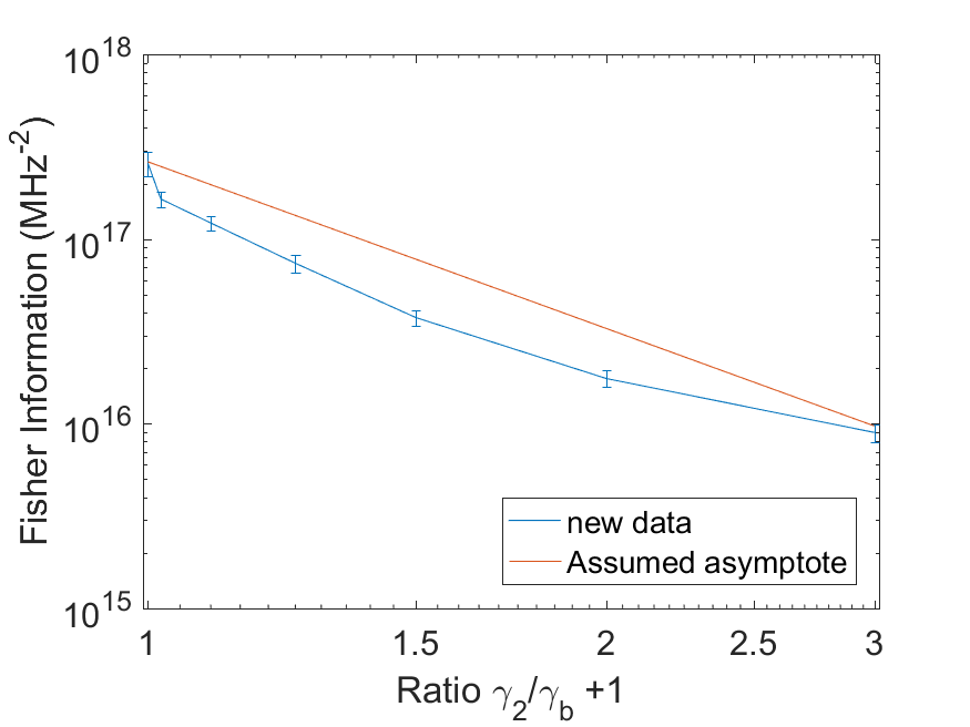
We numerically investigated the minimum difference between our protocol and the Heisenberg limit, which can only be achieved given full control over the nuclei in absence of decoherence $\gamma_{2}=0$ .

Figure 5 shows the maximum ratio between the Fisher Information of the investigated protocol and the Heisenberg limit. For different coupling strength the ratio is independent of the number of nuclei. Note that the peaks are due to the monte carlo simulation. This is confirmed by the curves on the right hand side of figure 5, where the maxima are found at $N\approx\beta^{-2}$ as expected.

Appendix D Simulation

The normal simulation (without making use of the permutation invariance) repeats the following steps (after initializing the nuclear spins to $\ket{\psi_{0}}=\ket{+}^{\otimes M}$ , $\rho_{0}=\ket{\psi_{0}}\bra{\psi_{0}}$ )

1.

Simulate nuclear spin evolution with the operator

$U_{\mathrm{free}}=\exp\left(-i\delta\tau_{m}\sum_{m}\sigma_{z}^{(m)}/2\right)$ (60)

where $\tau_{m}$ is the time between two measurements.

Determine probability to measure the NV in $\ket{+_{y}}$ after preparing it in $\ket{+}$ and evolving it with the nuclear spins according to (5) by

	$\displaystyle p$	$\displaystyle=\mathrm{Tr}\left[\ket{+_{y}}\bra{+_{y}}\otimes\mathbbm{1}^{\otimes M}U\ket{+}\bra{+}\otimes\rho_{n}U^{\dagger}\right]=\mathrm{Tr}\left[U_{+}\rho_{n}U_{+}^{\dagger}\right]$		(61)
		$\displaystyle=\bra{\psi_{n}}U_{+}^{\dagger}U_{+}\ket{\psi_{n}}\text{(for pure states)}$		(62)

where $U_{+}=\bra{+_{y}}U\otimes\mathbbm{1}^{\otimes M}\ket{+}$

3.

Probabilistically choose result according to $p$ , save result and evolve accordingly including normalisation $\rho_{n+1}=\mathcal{N}U_{+/-}\rho_{n}U_{+/-}^{\dagger}$ .

By using the subspace resulting from the symmetry in the case of many spins with equal coupling strength, many spins can be simulated efficiently, as this subspace has dimension $M+1$ instead of $2^{M}$ .

The Fisher Information

I_{N}=\sum\limits_{X^{N}}p_{X}\frac{1}{p_{X}^{2}}\left(\frac{\partial p_{X}}{\partial\delta}\right)^{2}

(63)

was calculated numerically for many different runs evolving $\rho$ following the recipe above to determine $p_{X}$ Evolving $\rho_{2/3}$ according to the same measurement outcomes as $\rho$ , but with a different evolution parameter $\delta\pm\mathrm{d}\delta$ allows to determine

\left(\frac{\partial p_{X}}{\partial\delta}\right)=\frac{p_{X}(\delta+\mathrm{d}\delta)-p_{X}(\delta-\mathrm{d}\delta)}{2\mathrm{d}\delta}

(64)

for many measurement records. After calculating the Fisher Information for every measurement record, the average and standard deviation can be obtained

The accuracy is limited by the Fisher Information due to the Cramer-Rao bound

\delta\omega_{N}\geq\frac{1}{\sqrt{I_{N}}}.

(65)

For pure states, the Logarithmic negativity can be simplified to an expression depending on the Schmidt coefficients $\alpha_{i}$ :

\displaystyle LN(\ket{\Psi}\bra{\Psi})=2\log\left(\sum\limits_{i}\alpha_{i}\right),

(66)

which can be calculated for considerably larger systems than the partial trace.

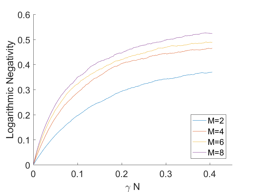
In order to obtain some insights into the entanglement buildup and its potential role as a resource in the metrology scheme, we use the logarithmic negativity Plenio 2005 as a quantifier of the entanglement between one of the auxiliary spins with the remaining $M-1$ spins and between equal bi-partitions of the auxiliary spins. While the entanglement between the nuclei builds up to a steady state after a time $\penalty\ 1/\gamma_{b}$ , it does not contribute to the quadratic scaling with the number of auxiliary spins as this effect is related to the readout process, nor does it support the $N^{3}$ super-Heisenberg scaling. However, destroying the entanglement after every measurement would lead to lower prefactor in the asymptotic SQL scaling as it inevitably leads to destruction of information. Figure 6 shows this buildup of entanglement of a scale of $N_{opt}\approx\left({2k_{0}T_{s}}/{\pi}\right)^{-2}=1/\gamma_{b}$ .