跳到论文正文
W Papers独立论文阅读器 arXiv:1905.12332 论文正文 计算阅读时间 · 0%
引用这篇论文根据当前论文元数据生成,正式投稿前建议核对。


License: arXiv.org perpetual non-exclusive license
arXiv:1905.12332v1 [quant-ph] 29 May 2019

One-Shot Quantum State Exchange

Yonghae Lee Email: yonghaelee@khu.ac.kr Affiliation:  Department of Mathematics and Research Institute for Basic Sciences, Kyung Hee University, Seoul 02447, Korea    Hayata Yamasaki Email: yamasaki@qi.t.u-tokyo.ac.jp Affiliation:  Photon Science Center, Graduate School of Engineering, The University of Tokyo, Bunkyo-ku, Tokyo 113-8656, Japan    Gerardo Adesso Email: gerardo.adesso@nottingham.ac.uk Affiliation:  School of Mathematical Sciences and Centre for the Mathematics and Theoretical Physics of Quantum Non-Equilibrium Systems, University of Nottingham, University Park, Nottingham NG7 2RD, United Kingdom    Soojoon Lee Email: level@khu.ac.kr Affiliation:  Department of Mathematics and Research Institute for Basic Sciences, Kyung Hee University, Seoul 02447, Korea Affiliation:  School of Mathematical Sciences and Centre for the Mathematics and Theoretical Physics of Quantum Non-Equilibrium Systems, University of Nottingham, University Park, Nottingham NG7 2RD, United Kingdom
August 11, 2026
Abstract

The quantum state exchange is a quantum communication task in which two users exchange their respective quantum information in the asymptotic setting. In this work, we consider a one-shot version of the quantum state exchange task, in which the users hold a single copy of the initial state, and they exchange their parts of the initial state by means of entanglement-assisted local operations and classical communication. We first derive lower bounds on the least amount of entanglement required for carrying out this task, and provide conditions on the initial state such that the protocol succeeds with zero entanglement cost. Based on these results, we reveal two counter-intuitive phenomena in this task, which make it different from a conventional SWAP operation. One tells how the users deal with their symmetric information in order to reduce the entanglement cost. The other shows that it is possible for the users to gain extra shared entanglement after this task.

pacs
03.67.Hk, 89.70.Cf, 03.67.Mn

Introduction.— In quantum information theory, the quantum state exchange Oppenheim and Winter; Lee et al. 2019 is a quantum communication task, in which two users, Alice and Bob, exchange their quantum information by means of local operations and classical communication (LOCC) assisted by shared entanglement. A main research aim in the study of the quantum state exchange is to evaluate the least amount of entanglement needed for the task, as in other quantum communication tasks, such as quantum state merging Horodecki et al. 2005; Horodecki et al. 2006 and quantum state redistribution Devetak and Yard 2008; Yard and Devetak 2009.

Most quantum communication tasks Schumacher 1995; Horodecki et al. 2005; Horodecki et al. 2006; Devetak and Yard 2008; Yard and Devetak 2009; Abeyesinghe et al. 2009 including the quantum state exchange usually assume the asymptotic scenario, in which users can have an unbounded number of independent and identically distributed copies of an initial state, and they carry out their task with the copies. On the other hand, it is not easy in a realistic situation to prepare a sufficiently large number of state copies, and the amount of non-local resources available for the users is limited. To reflect these practical difficulties, quantum information research has focused more recently on the one-shot scenario Berta et al. 2011; Renes and Renner 2012; Wang and Renner 2012; Datta and Hsieh 2013; Berta et al. 2016; Zhao et al. 2018; Anshu et al. 2018; Regula et al. 2018; Yamasaki and Murao.

In this work, we introduce and study the one-shot quantum state exchange (OSQSE) task. This is not only a useful quantum communication task, but can also have a potential application in quantum computation. Let us consider a specific situation as follows. Alice and Bob want to carry out the SWAP gate Nielsen and Chuang 2010, which plays an important role in universal quantum computation Jozsa and Miyake 2008. The problem is that they cannot directly apply the SWAP gate, because they are far apart. If Alice and Bob are sharing prior entanglement, then the OSQSE can be a method to non-locally perform the SWAP gate, as both operationally provide the same result. However, the OSQSE has unique properties which we reveal in this work.

We formally define the OSQSE and its optimal entanglement cost, and derive computable lower bounds on the latter, which in turn yield bounds for the asymptotic quantum state exchange Oppenheim and Winter; Lee et al. 2019. In addition, we provide two useful conditions to decide whether a given initial state enables OSQSE with zero entanglement cost. We then show that there exist counter-intuitive phenomena in the OSQSE task that set it apart from the conventional SWAP operation.

One-shot quantum state exchange.— Consider two users, Alice and Bob, holding parts AA and BB of the initial state |ψ⟩≡|ψ⟩A1​B1​A2​B2​R\ket{\psi}\equiv\ket{\psi}_{A_{1}B_{1}A_{2}B_{2}R} with systems A=A1​A2A=A_{1}A_{2} and B=B1​B2B=B_{1}B_{2}, respectively. Alice’s and Bob’s goal is either to exchange their parts A1A_{1} and B1B_{1} or to exchange their whole parts AA and BB.

Specifically, let ψf1\psi_{f_{1}} and ψf12\psi_{f_{12}} be the final states of the task,

ψf1\displaystyle\psi_{f_{1}} =\displaystyle= (𝟙A1→A1′⊗𝟙B1→B1′⊗𝟙A2​B2​R)​(ψ),\displaystyle\big(\mathds{1}_{A_{1}\to A^{\prime}_{1}}\otimes\mathds{1}_{B_{1}\to B^{\prime}_{1}}\otimes\mathds{1}_{A_{2}B_{2}R}\big)(\psi),
ψf12\displaystyle\psi_{f_{12}} =\displaystyle= (𝟙A→A′⊗𝟙B→B′⊗𝟙R)​(ψ),\displaystyle\big(\mathds{1}_{A\to A^{\prime}}\otimes\mathds{1}_{B\to B^{\prime}}\otimes\mathds{1}_{R}\big)(\psi),

where ψ=|ψ⟩​⟨ψ|\psi=\ket{\psi}\bra{\psi}, and the dimension of system X′X^{\prime} is identical to that of system XX. Note that B1′B^{\prime}_{1}, B′B^{\prime} and A1′A^{\prime}_{1}, A′A^{\prime} are Alice’s and Bob’s systems, respectively. Then three joint operations

ℰψ,K,L1:A1​EAin⊗B1​EBin⟶B1′​EAout⊗A1′​EBout,\displaystyle\mathcal{E}_{\psi,K,L}^{1}:A_{1}E_{\mathrm{A}}^{\mathrm{in}}\otimes B_{1}E_{\mathrm{B}}^{\mathrm{in}}\longrightarrow B^{\prime}_{1}E_{\mathrm{A}}^{\mathrm{out}}\otimes A^{\prime}_{1}E_{\mathrm{B}}^{\mathrm{out}},
ℰψ,K,L1|2:A​EAin⊗B​EBin⟶B1′​A2​EAout⊗A1′​B2​EBout,\displaystyle\mathcal{E}_{\psi,K,L}^{1|2}:AE_{\mathrm{A}}^{\mathrm{in}}\otimes BE_{\mathrm{B}}^{\mathrm{in}}\longrightarrow B^{\prime}_{1}A_{2}E_{\mathrm{A}}^{\mathrm{out}}\otimes A^{\prime}_{1}B_{2}E_{\mathrm{B}}^{\mathrm{out}}, (1)
ℰψ,K,L12:A​EAin⊗B​EBin⟶B′​EAout⊗A′​EBout,\displaystyle\mathcal{E}_{\psi,K,L}^{12}:AE_{\mathrm{A}}^{\mathrm{in}}\otimes BE_{\mathrm{B}}^{\mathrm{in}}\longrightarrow B^{\prime}E_{\mathrm{A}}^{\mathrm{out}}\otimes A^{\prime}E_{\mathrm{B}}^{\mathrm{out}},

are called the OSQSE protocols of |ψ⟩\ket{\psi}, if they are performed by LOCC between Alice and Bob, and satisfy

ψf1⊗Φ\displaystyle\psi_{f_{1}}\otimes{\Phi} =\displaystyle= (ℰψ,K,L1⊗𝟙A2​B2​R)​(ψ⊗Ψ)\displaystyle\left(\mathcal{E}_{\psi,K,L}^{1}\otimes\mathds{1}_{A_{2}B_{2}R}\right)\left(\psi\otimes{\Psi}\right) (2)
=\displaystyle= (ℰψ,K,L1|2⊗𝟙R)​(ψ⊗Ψ),\displaystyle\left(\mathcal{E}_{\psi,K,L}^{1|2}\otimes\mathds{1}_{R}\right)\left(\psi\otimes{\Psi}\right),
ψf12⊗Φ\displaystyle\psi_{f_{12}}\otimes{\Phi} =\displaystyle= (ℰψ,K,L12⊗𝟙R)​(ψ⊗Ψ),\displaystyle\left(\mathcal{E}_{\psi,K,L}^{12}\otimes\mathds{1}_{R}\right)\left(\psi\otimes{\Psi}\right),

where Ψ{\Psi} and Φ{\Phi} are pure maximally entangled states with Schmidt rank KK and LL on systems EAin​EBinE_{\mathrm{A}}^{\mathrm{in}}E_{\mathrm{B}}^{\mathrm{in}} and EAout​EBoutE_{\mathrm{A}}^{\mathrm{out}}E_{\mathrm{B}}^{\mathrm{out}}, respectively. It is possible to generalize the above definitions by adding errors for approximation to Eq. (2), but it suffices to only consider error-free protocols to obtain our main results.

At this point, it is instructive to inform differences among the three protocols in Eq. (One-Shot Quantum State Exchange) as follows: The first two protocols ℰψ,K,L1\mathcal{E}_{\psi,K,L}^{1} and ℰψ,K,L1|2\mathcal{E}_{\psi,K,L}^{1|2} indicate that only the parts A1A_{1} and B1B_{1} are exchanged, while the whole parts A1​A2A_{1}A_{2} and B1​B2B_{1}B_{2} are exchanged in the third protocol ℰψ,K,L12\mathcal{E}_{\psi,K,L}^{12}. In addition, the parts A2A_{2} and B2B_{2} can be used for exchanging A1A_{1} and B1B_{1} in the protocol ℰψ,K,L1|2\mathcal{E}_{\psi,K,L}^{1|2}, while A2A_{2} and B2B_{2} are untouched in the protocol ℰψ,K,L1\mathcal{E}_{\psi,K,L}^{1}.

Depending on the types of OSQSE protocols, we define three optimal entanglement costs

𝐞A1↔B1​(ψ)\displaystyle\mathbf{e}_{A_{1}\leftrightarrow B_{1}}\left(\psi\right) =\displaystyle= infℰψ,K,L1(log⁡K−log⁡L),\displaystyle\inf_{\mathcal{E}_{\psi,K,L}^{1}}\left(\log K-\log L\right),
𝐞A1↔B1A2​B2​(ψ)\displaystyle\mathbf{e}_{A_{1}\leftrightarrow B_{1}}^{A_{2}B_{2}}\left(\psi\right) =\displaystyle= infℰψ,K,L1|2(log⁡K−log⁡L),\displaystyle\inf_{\mathcal{E}_{\psi,K,L}^{1|2}}\left(\log K-\log L\right), (3)
𝐞A↔B​(ψ)\displaystyle\mathbf{e}_{A\leftrightarrow B}\left(\psi\right) =\displaystyle= infℰψ,K,L12(log⁡K−log⁡L),\displaystyle\inf_{\mathcal{E}_{\psi,K,L}^{12}}\left(\log K-\log L\right),

where the quantity log⁡K−log⁡L\log K-\log L is called the entanglement cost of the OSQSE protocol, and the infimums are taken over all joint protocols ℰψ,K,L1\mathcal{E}_{\psi,K,L}^{1}, ℰψ,K,L1|2\mathcal{E}_{\psi,K,L}^{1|2}, and ℰψ,K,L12\mathcal{E}_{\psi,K,L}^{12}, respectively.

By the definitions of the optimal entanglement costs, we obtain the following proposition.

Proposition 1.

For any input state ψ\psi, 𝐞A1↔B1​(ψ)≥𝐞A1↔B1A2​B2​(ψ)\mathbf{e}_{A_{1}\leftrightarrow B_{1}}\left(\psi\right)\geq\mathbf{e}_{A_{1}\leftrightarrow B_{1}}^{A_{2}B_{2}}\left(\psi\right).

Converse bounds.— A real number rr is called a converse bound of the optimal entanglement cost if it is upper bounded by the entanglement cost of any OSQSE protocol. We derive converse bounds of the optimal entanglement costs as follows.

As in the asymptotic scenario Oppenheim and Winter; Lee et al. 2019, we consider a one-shot version of the RR-assisted quantum state exchange task, in which the reference system RR is divided into two systems RAR_{\mathrm{A}} and RBR_{\mathrm{B}}, and then Alice and Bob receive the divided parts RAR_{\mathrm{A}} and RBR_{\mathrm{B}}, respectively, so that the initial state |ψ~⟩A1​B1​A2​B2​RA​RB\ket{\tilde{\psi}}_{A_{1}B_{1}A_{2}B_{2}R_{\mathrm{A}}R_{\mathrm{B}}} is divided into Alice’s parts A​RAAR_{\mathrm{A}} and Bob’s parts B​RBBR_{\mathrm{B}}. This can be realized by using a quantum channel 𝒩:R⟶RA\mathcal{N}:R\longrightarrow R_{\mathrm{A}} and its complementary channel 𝒩c:R⟶RB\mathcal{N}^{c}:R\longrightarrow R_{\mathrm{B}} Wilde 2013. Let ℰψ~,K,L\mathcal{E}_{\tilde{\psi},K,L} be an RR-assisted OSQSE protocol,

ℰψ~,K,L:A​RA​EAin⊗B​RB​EBin⟶B1′​A2​RA​EAout⊗A1′​B2​RB​EBout,\mathcal{E}_{\tilde{\psi},K,L}:AR_{\mathrm{A}}E_{\mathrm{A}}^{\mathrm{in}}\otimes BR_{\mathrm{B}}E_{\mathrm{B}}^{\mathrm{in}}\longrightarrow B^{\prime}_{1}A_{2}R_{\mathrm{A}}E_{\mathrm{A}}^{\mathrm{out}}\otimes A^{\prime}_{1}B_{2}R_{\mathrm{B}}E_{\mathrm{B}}^{\mathrm{out}},

with the entanglement cost log⁡K−log⁡L\log K-\log L such that ψ~f⊗Φ=ℰψ~,K,L​(ψ~⊗Ψ)\tilde{\psi}_{f}\otimes{\Phi}=\mathcal{E}_{\tilde{\psi},K,L}(\tilde{\psi}\otimes{\Psi}), where ψ~f=(𝟙A1→A1′⊗𝟙B1→B1′⊗𝟙A2​B2​RA​RB)​(ψ~)\tilde{\psi}_{f}=(\mathds{1}_{A_{1}\to A^{\prime}_{1}}\otimes\mathds{1}_{B_{1}\to B^{\prime}_{1}}\otimes\mathds{1}_{A_{2}B_{2}R_{\mathrm{A}}R_{\mathrm{B}}})(\tilde{\psi}). Note that ℰψ~,K,L\mathcal{E}_{\tilde{\psi},K,L} is an LOCC protocol by Alice and Bob. Let σM\sigma^{M} be the maximally mixed state with rank MM. From the majorization condition for LOCC convertibility Nielsen 1999; Mari et al. 2014, the state ρB1′​A2​RA⊗σEBoutL\rho_{B^{\prime}_{1}A_{2}R_{\mathrm{A}}}\otimes\sigma^{L}_{E_{\mathrm{B}}^{\mathrm{out}}} majorizes the state ρA​RA⊗σEBinK\rho_{AR_{\mathrm{A}}}\otimes\sigma^{K}_{E_{\mathrm{B}}^{\mathrm{in}}}. Let FF be an additive and Schur concave function van Dam and Hayden such that F⁡(σM)=log⁡MF(\sigma^{M})=\log M for any MM. From the Schur concavity of the function FF, the inequality F⁡(ρB1′​A2​RA⊗σEBoutL)≤F⁡(ρA​RA⊗σEBinK)F(\rho_{B^{\prime}_{1}A_{2}R_{\mathrm{A}}}\otimes\sigma^{L}_{E_{\mathrm{B}}^{\mathrm{out}}})\leq F(\rho_{AR_{\mathrm{A}}}\otimes\sigma^{K}_{E_{\mathrm{B}}^{\mathrm{in}}}) holds. Since FF is additive and ρB1′​A2​RA=ρB1​A2​RA\rho_{B^{\prime}_{1}A_{2}R_{\mathrm{A}}}=\rho_{B_{1}A_{2}R_{\mathrm{A}}}, it follows that log⁡K−log⁡L≥F⁡(ρB1​A2​RA)−F⁡(ρA​RA)\log K-\log L\geq F(\rho_{B_{1}A_{2}R_{\mathrm{A}}})-F(\rho_{AR_{\mathrm{A}}}). Since any protocol ℰψ,K,L1|2\mathcal{E}_{\psi,K,L}^{1|2} is also an RR-assisted OSQSE protocol for the initial state |ψ⟩\ket{\psi}, we obtain the following theorem.

Theorem 2.

For any input state ψ\psi, the optimal entanglement cost 𝐞A1↔B1A2​B2​(ψ)\mathbf{e}_{A_{1}\leftrightarrow B_{1}}^{A_{2}B_{2}}\left(\psi\right) is lower bounded by

l1|2​(ψ)=supF,𝒩[F⁡(𝒩​(ψ)B1​A2​RA)−F⁡(𝒩​(ψ)A​RA)],l_{1|2}(\psi)=\sup_{F,\mathcal{N}}\left[F(\mathcal{N}(\psi)_{B_{1}A_{2}R_{\mathrm{A}}})-F(\mathcal{N}(\psi)_{AR_{\mathrm{A}}})\right],

where FF is an additive and Schur concave function such that F⁡(σM)=log⁡MF(\sigma^{M})=\log M for any MM and 𝒩⁡(ρ)\mathcal{N}(\rho) is a quantum channel from RR to RAR_{\mathrm{A}}.

In Theorem 2, if RR is directly sent to either Alice or Bob without splitting, and we restrict the function FF to the quantum Rényi entropy Sα​(ϱ)S_{\alpha}(\varrho) of order α\alpha van Dam and Hayden for a quantum state ϱ\varrho, then we obtain the following computable converse bounds.

Corollary 3.

For any input state ψ\psi, 𝐞A1↔B1A2​B2​(ψ)≥l1|2c​(ψ)=maxα∈[0,∞]⁡fψ​(α)\mathbf{e}_{A_{1}\leftrightarrow B_{1}}^{A_{2}B_{2}}\left(\psi\right)\geq l_{1|2}^{c}(\psi)=\max_{\alpha\in[0,\infty]}f_{\psi}(\alpha),where fψ​(α)f_{\psi}(\alpha) is a function of |ψ⟩\ket{\psi} and α\alpha defined by fψ​(α)=max⁡{Sα​(ρA1​B2)−Sα​(ρB),Sα​(ρB1​A2)−Sα​(ρA)}f_{\psi}(\alpha)=\max\{S_{\alpha}(\rho_{A_{1}B_{2}})-S_{\alpha}(\rho_{B}),S_{\alpha}(\rho_{B_{1}A_{2}})-S_{\alpha}(\rho_{A})\}.

We refer the reader to Appendix A for the proof of Corollary 3. Remark that the converse bound l1|2cl_{1|2}^{c} can be easily computed by means of analytical or numerical methods, since the function fψ​(α)f_{\psi}(\alpha) is one-variable and differentiable on (0,∞)(0,\infty). For the different types of the OSQSE protocols, we can also obtain a similar computable converse bound as follows:

𝐞X↔Y​(ψ)≥maxα∈[0,∞]⁡|Sα​(ρX)−Sα​(ρY)|,\mathbf{e}_{X\leftrightarrow Y}\left(\psi\right)\geq\max_{\alpha\in[0,\infty]}\left|S_{\alpha}(\rho_{X})-S_{\alpha}(\rho_{Y})\right|, (4)

where the pair (X,Y)(X,Y) can refer either to (A1,B1)(A_{1},B_{1}) or to (A,B)(A,B).

We also remark that in Theorem 2, if FF is chosen as the von Neumann entropy Wilde 2013, then the converse bound l1|2l_{1|2} recovers a theoretical converse bound in Refs. Oppenheim and Winter; Lee et al. 2019. In addition, a computable converse bound therein is just fψ​(1)f_{\psi}(1) in Corollary 3. By virtue of the additivity of FF, it is clear that l1|2l_{1|2} and l1|2cl_{1|2}^{c} are also converse bounds of the optimal entanglement cost for the asymptotic quantum state exchange task. Hence, our converse bounds improve the existing bounds in Refs. Oppenheim and Winter; Lee et al. 2019. For example, if the initial state |ψ1⟩≡|ψ1⟩A1​B1​A2​B2​R\ket{\psi_{1}}\equiv\ket{\psi_{1}}_{A_{1}B_{1}A_{2}B_{2}R} is

|ψ1⟩=15​|00000⟩+350​|00010⟩+35​|01001⟩+2750​|11100⟩,\ket{\psi_{1}}=\mbox{$\frac{1}{5}\ket{00000}+\sqrt{\frac{3}{50}}\ket{00010}+\frac{3}{5}\ket{01001}+\sqrt{\frac{27}{50}}\ket{11100}$}, (5)

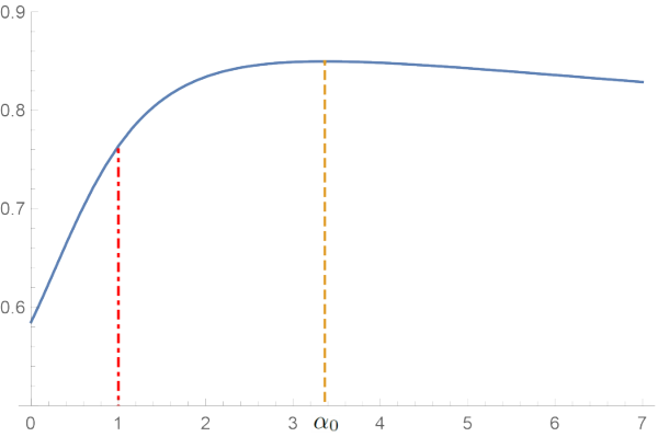
then we can find a value α0∈[0,∞]\alpha_{0}\in[0,\infty] such that l1|2c​(ψ1)=fψ1​(α0)>fψ1​(1)l_{1|2}^{c}(\psi_{1})=f_{\psi_{1}}(\alpha_{0})>f_{\psi_{1}}(1) as depicted in Fig. 1. This example shows that our bound l1|2c​(ψ)l_{1|2}^{c}(\psi) is tighter than the existing bound fψ​(1)f_{\psi}(1).

Refer to caption
Figure 1: The graph of the function fψ1​(α)f_{\psi_{1}}(\alpha) for a specific initial state |ψ1⟩\ket{\psi_{1}} in Eq. (5). The maximum of fψ1​(α)f_{\psi_{1}}(\alpha) is attained at the point α0\alpha_{0} (≈3.362)(\approx 3.362). In the graph, α0\alpha_{0} is represented as the yellow dashed line, and 1 is represented as the red dashed dotted line.

Conditions for zero entanglement cost.— We now present conditions for OSQSE with zero entanglement cost.

By the converse bound in Eq. (4), it is obvious that if there exist Alice’s and Bob’s local isometries performing the OSQSE task, then the optimal entanglement cost is zero. We first characterize this type of strategy. Let (X,Y)(X,Y) be a pair of two systems, which can be either (A1,B1)(A_{1},B_{1}) or (A,B)(A,B), and consider a spectral decomposition of the reduced state ρX​Y\rho_{XY} for |ψ⟩\ket{\psi}, ρX​Y=∑i=1Nλi​|ξi⟩​⟨ξi|X​Y\rho_{XY}=\sum_{i=1}^{N}\lambda_{i}\ket{\xi_{i}}\bra{\xi_{i}}_{XY}, where λi>0\lambda_{i}>0 with ∑i=1Nλi=1\sum_{i=1}^{N}\lambda_{i}=1. For each ii, we define the matrix ΩX​Yi​(ψ)\Omega_{XY}^{i}(\psi) by

ΩX​Yi​(ψ)=∑j,k(⟨j|X⊗⟨k|Y)​|ξi⟩X​Y​|j⟩​⟨k|,\Omega_{XY}^{i}(\psi)=\sum_{j,k}\left(\bra{j}_{X}\otimes\bra{k}_{Y}\right)\ket{\xi_{i}}_{XY}\ket{j}\bra{k},

where {|j⟩}\{\ket{j}\} and {|k⟩}\{\ket{k}\} indicate the computational bases on Alice’s and Bob’s systems, respectively. Then we obtain the following sufficient condition.

Theorem 4.

Let (X,Y)(X,Y) be either (A1,B1)(A_{1},B_{1}) or (A,B)(A,B). If there exist isometries UU and VV such that, for each ii, (ΩX​Yi​(ψ))t=U​ΩX​Yi​(ψ)​V{\left(\Omega_{XY}^{i}(\psi)\right)}^{t}=U\Omega_{XY}^{i}(\psi)V, then 𝐞X↔Y​(ψ)=0\mathbf{e}_{X\leftrightarrow Y}\left(\psi\right)=0.

Here, the isometries UU and VV indicate Alice’s and Bob’s local operations exchanging the parts XX and YY without shared entanglement. The proof of Theorem 4 is in Appendix B.

From the converse bound in Eq. (4), observe that if the spectrum of Alice’s state is different from that of Bob’s state, then the optimal entanglement cost cannot be zero. Based on this observation, we obtain the following theorem, whose proof can be found in Appendix C.

Theorem 5.

Let (X,Y)(X,Y) be either (A1,B1)(A_{1},B_{1}) or (A,B)(A,B). If 𝐞X↔Y​(ψ)=0\mathbf{e}_{X\leftrightarrow Y}\left(\psi\right)=0, then there exists an isometry UX→YU_{X\rightarrow Y} such that ρY=UX→Y​ρX​(UX→Y)†\rho_{Y}=U_{X\rightarrow Y}\rho_{X}(U_{X\rightarrow Y})^{\dagger}.

We remark that the converse of Theorem 5 is not true in general. Let us consider the following simple initial state

|ψ2⟩A1​B1​A2​B2=12​(|0000⟩+|0101⟩+|1010⟩+|1111⟩),\ket{\psi_{2}}_{A_{1}B_{1}A_{2}B_{2}}=\mbox{$\frac{1}{2}\left(\ket{0000}+\ket{0101}+\ket{1010}+\ket{1111}\right)$},

then 𝐞A1↔B1​(ψ2)≥𝐞A1↔B1A2​B2​(ψ2)≥2\mathbf{e}_{A_{1}\leftrightarrow B_{1}}\left(\psi_{2}\right)\geq\mathbf{e}_{A_{1}\leftrightarrow B_{1}}^{A_{2}B_{2}}\left(\psi_{2}\right)\geq 2, from Proposition 1 and Corollary 3. However, the state |ψ2⟩\ket{\psi_{2}} satisfies the necessary condition in Theorem 5, since its reduced states ρA1\rho_{A_{1}} and ρB1\rho_{B_{1}} are identical.

Counter-intuitive phenomena.— We are now in the position to present two phenomena which show the important differences between the OSQSE task and the SWAP operation.

(1) Symmetric information.— For the initial state |ψ⟩\ket{\psi}, let us consider a scenario in which Alice and Bob exchange their whole information AA and BB. Assume that their parts A2A_{2} and B2B_{2} are symmetric, while the remaining parts A1A_{1} and B1B_{1} are not symmetric, i.e., the initial state |ψ⟩\ket{\psi} satisfies (SWAPA1↔B1)​(ψ)≠ψ\left(\mathrm{SWAP}_{A_{1}\leftrightarrow B_{1}}\right)\left(\psi\right)\neq\psi and (SWAPA2↔B2)​(ψ)=ψ\left(\mathrm{SWAP}_{A_{2}\leftrightarrow B_{2}}\right)\left(\psi\right)=\psi where SWAPX↔Y\mathrm{SWAP}_{X\leftrightarrow Y} is the operation swapping quantum states in systems XX and YY.

From a viewpoint of the SWAP operation, if Alice and Bob want to exchange AA and BB, then it suffices for them to exchange A1A_{1} and B1B_{1}, since A2A_{2} is identical to B2B_{2}. This situation can be more easily understood by using a cargo exchange as a metaphor for the SWAP operation as depicted in Fig. 2. In the cargo exchange, assume that Alice and Bob want to exchange their whole cargoes, and some of the cargoes are symmetric. In terms of efficiency, it is reasonable for them to exchange only A1A_{1} and B1B_{1} in order to reduce the cargo exchange cost, because the cargoes A2A_{2} and B2B_{2} are the same.

Refer to caption
Figure 2: Illustration of the cargo exchange task. The cargoes A1​A2A_{1}A_{2} and B1​B2B_{1}B_{2} belong to Alice and Bob, respectively. Assume that the cargoes A2A_{2} and B2B_{2} are symmetric, but A1A_{1} and B1B_{1} are not symmetric. When Alice and Bob exchange their whole cargoes A1​A2A_{1}A_{2} and B1​B2B_{1}B_{2}, it suffices for them to exchange A1A_{1} and B1B_{1}, since A2A_{2} is identical to B2B_{2}. The truck indicates the cost needed for exchanging A1A_{1} and B1B_{1}.

On the other hand, in the OSQSE, the proper use of the symmetric parts A2A_{2} and B2B_{2} can more efficiently reduce the entanglement cost compared to exchanging only A1A_{1} and B1B_{1} without using A2A_{2} and B2B_{2}. To be specific, there exists an initial state |ψ⟩\ket{\psi} such that the parts A2A_{2} and B2B_{2} are symmetric and 𝐞A↔B​(ψ)=0\mathbf{e}_{A\leftrightarrow B}\left(\psi\right)=0 while the rest parts A1A_{1} and B1B_{1} are not symmetric. Consider the specific initial state

|ϕ1⟩A1​B1​A2​B2​R=12​(|00000⟩+|01111⟩),\ket{\phi_{1}}_{A_{1}B_{1}A_{2}B_{2}R}=\mbox{$\frac{1}{\sqrt{2}}\left(\ket{00000}+\ket{01111}\right)$},

where A2A_{2} and B2B_{2} are symmetric but A1A_{1} and B1B_{1} are not. Since ΩA​B1​(ϕ1)=|00⟩​⟨00|\Omega_{AB}^{1}(\phi_{1})=\ket{00}\bra{00} and ΩA​B2​(ϕ1)=|01⟩​⟨11|\Omega_{AB}^{2}(\phi_{1})=\ket{01}\bra{11}, we can show that ΩA​B1​(ϕ1)\Omega_{AB}^{1}(\phi_{1}) and ΩA​B2​(ϕ1)\Omega_{AB}^{2}(\phi_{1}) satisfy the condition in Theorem 4, by setting

U=V=|00⟩​⟨00|+|01⟩​⟨11|+|10⟩​⟨10|+|11⟩​⟨01|.U=V=\ket{00}\bra{00}+\ket{01}\bra{11}+\ket{10}\bra{10}+\ket{11}\bra{01}. (6)

Thus we obtain that 𝐞A↔B​(ϕ1)=0\mathbf{e}_{A\leftrightarrow B}\left(\phi_{1}\right)=0, which means that AA and BB can be exchanged by means of LOCC without consuming any non-local resource. As mentioned above, this phenomenon cannot occur when using the SWAP operation.

The above example also shows that the use of the symmetric parts A2A_{2} and B2B_{2} can reduce the entanglement cost for exchanging A1A_{1} and B1B_{1}. Since the initial state |ϕ1⟩\ket{\phi_{1}} does not satisfy the necessary condition in Theorem 5, we obtain 𝐞A1↔B1​(ϕ1)>0\mathbf{e}_{A_{1}\leftrightarrow B_{1}}\left(\phi_{1}\right)>0. Observe that the isometry UU (VV) in Eq. (6) represents Alice’s (Bob’s) local operation CNOTA\mathrm{CNOT}_{\mathrm{A}} (CNOTB\mathrm{CNOT}_{\mathrm{B}}) whose target and controlled systems are A1A_{1} (B1B_{1}) and A2A_{2} (B2B_{2}), respectively. This implies that Alice and Bob can exchange A1A_{1} and B1B_{1} by using local operations. It follows that 0≥𝐞A1↔B1A2​B2​(ϕ1)0\geq\mathbf{e}_{A_{1}\leftrightarrow B_{1}}^{A_{2}B_{2}}\left(\phi_{1}\right). In fact, 𝐞A1↔B1A2​B2​(ϕ1)=0\mathbf{e}_{A_{1}\leftrightarrow B_{1}}^{A_{2}B_{2}}\left(\phi_{1}\right)=0 from Corollary 3. Therefore, we obtain 𝐞A1↔B1​(ϕ1)>𝐞A1↔B1A2​B2​(ϕ1)\mathbf{e}_{A_{1}\leftrightarrow B_{1}}\left(\phi_{1}\right)>\mathbf{e}_{A_{1}\leftrightarrow B_{1}}^{A_{2}B_{2}}\left(\phi_{1}\right).

When A2A_{2} and B2B_{2} are symmetric, we can show the following relation between the optimal entanglement costs by definition.

Proposition 6.

𝐞A↔B​(ψ)=𝐞A1↔B1A2​B2​(ψ)\mathbf{e}_{A\leftrightarrow B}\left(\psi\right)=\mathbf{e}_{A_{1}\leftrightarrow B_{1}}^{A_{2}B_{2}}\left(\psi\right), if the parts A2A_{2} and B2B_{2} of |ψ⟩\ket{\psi} are symmetric.

From Proposition 6, we can see that, when Alice and Bob exchange systems AA and BB of |ψ⟩\ket{\psi} with symmetric parts A2A_{2} and B2B_{2}, they can achieve the optimal entanglement cost by exchanging only A1A_{1} and B1B_{1}, making the most of this symmetry.

(2) Negative entanglement cost.— As in the asymptotic quantum state exchange task Oppenheim and Winter; Lee et al. 2019, there exist initial states to show that the entanglement cost of the OSQSE task can be negative. Assume that Alice and Bob exchange the parts A1A_{1} and B1B_{1} of the initial state

|ϕ2⟩A1​B1​A2​B2=12​∑i,j=01|i⟩A1​|j⟩B1​|j⟩A2​|i⟩B2,\ket{\phi_{2}}_{A_{1}B_{1}A_{2}B_{2}}=\mbox{$\frac{1}{2}\sum_{i,j=0}^{1}\ket{i}_{A_{1}}\ket{j}_{B_{1}}\ket{j}_{A_{2}}\ket{i}_{B_{2}}$}, (7)

where |ϕ2⟩\ket{\phi_{2}} consists of two ebits |e⟩A1​B2\ket{e}_{A_{1}B_{2}} and |e⟩B1​A2\ket{e}_{B_{1}A_{2}}. To exchange A1A_{1} and B1B_{1}, both Alice and Bob prepare an ebit, respectively, and they locally implement entanglement swapping Żukowski et al. 1993 by performing two Bell measurements on A2A_{2}, B2B_{2}, and the parts of the ebits, as described in Fig. 3. Then they can exchange A1A_{1} and B1B_{1}, and can share two ebits at the same time. This means that the entanglement cost can be negative. In fact, we have 𝐞A1↔B1A2​B2​(ϕ2)=−2\mathbf{e}_{A_{1}\leftrightarrow B_{1}}^{A_{2}B_{2}}\left(\phi_{2}\right)=-2 from Corollary 3. This is in stark contrast with the SWAP operation, which cannot lead to creation of shared entanglement between Alice and Bob.

Refer to caption
Figure 3: Illustration of the one-shot quantum state exchange protocol of |ϕ2⟩\ket{\phi_{2}} in Eq. (7). (a) In order to exchange A1A_{1} and B1B_{1}, Alice and Bob locally prepare an ebit each, and they apply Bell measurements to the shaded areas. (b) By performing local operations corresponding to the measurement outcomes, the parts A1A_{1} and B1B_{1} can be exchanged. At the same time, Alice and Bob can share two ebits.

From Proposition 6, we can know that if A2A_{2} and B2B_{2} are symmetric, then 𝐞A1↔B1A2​B2​(ψ)\mathbf{e}_{A_{1}\leftrightarrow B_{1}}^{A_{2}B_{2}}\left(\psi\right) cannot be negative. One may ask the question: Is there any condition that implies the non-negativity of the optimal entanglement cost 𝐞A1↔B1A2​B2\mathbf{e}_{A_{1}\leftrightarrow B_{1}}^{A_{2}B_{2}}? To answer this question, we present the following inequalities.

Proposition 7.
𝐞A1↔B1A2​B2​(ψ)+𝐞B1′↔A1′A2​B2​(ψf1)\displaystyle\mathbf{e}_{A_{1}\leftrightarrow B_{1}}^{A_{2}B_{2}}(\psi)+\mathbf{e}_{B^{\prime}_{1}\leftrightarrow A^{\prime}_{1}}^{A_{2}B_{2}}(\psi_{f_{1}}) ≥\displaystyle\geq 0,\displaystyle 0,
𝐞A1↔B1A2​B2​(ψ)+𝐞A2↔B2B1′​A1′​(ψf1)\displaystyle\mathbf{e}_{A_{1}\leftrightarrow B_{1}}^{A_{2}B_{2}}(\psi)+\mathbf{e}_{A_{2}\leftrightarrow B_{2}}^{B^{\prime}_{1}A^{\prime}_{1}}(\psi_{f_{1}}) ≥\displaystyle\geq 𝐞A↔B​(ψ),\displaystyle\mathbf{e}_{A\leftrightarrow B}(\psi),

where 𝐞B1′↔A1′A2​B2​(ψf1)\mathbf{e}_{B^{\prime}_{1}\leftrightarrow A^{\prime}_{1}}^{A_{2}B_{2}}(\psi_{f_{1}}) is the optimal entanglement cost for exchanging B1′B^{\prime}_{1} and A1′A^{\prime}_{1} when using A2A_{2} and B2B_{2}, and 𝐞A2↔B2B1′​A1′​(ψf1)\mathbf{e}_{A_{2}\leftrightarrow B_{2}}^{B^{\prime}_{1}A^{\prime}_{1}}(\psi_{f_{1}}) is the optimal entanglement cost for exchanging A2A_{2} and B2B_{2} when using B1′B^{\prime}_{1} and A1′A^{\prime}_{1}.

In Proposition 7, the first inequality comes from the fact that Alice and Bob cannot increase the amount of entanglement between them by means of LOCC Vedral et al. 1997, while the second one is straightforward from the definitions of the optimal entanglement costs. From Proposition 7, we can see that if 𝐞B1′↔A1′A2​B2​(ψf1)\mathbf{e}_{B^{\prime}_{1}\leftrightarrow A^{\prime}_{1}}^{A_{2}B_{2}}(\psi_{f_{1}}) or 𝐞A2↔B2B1′​A1′​(ψf1)\mathbf{e}_{A_{2}\leftrightarrow B_{2}}^{B^{\prime}_{1}A^{\prime}_{1}}(\psi_{f_{1}}) is non-positive, then 𝐞A1↔B1A2​B2​(ψ)\mathbf{e}_{A_{1}\leftrightarrow B_{1}}^{A_{2}B_{2}}(\psi) cannot be negative. Moreover, if the condition 𝐞A2↔B2B1′​A1′​(ψf1)≤𝐞A↔B​(ψ)\mathbf{e}_{A_{2}\leftrightarrow B_{2}}^{B^{\prime}_{1}A^{\prime}_{1}}(\psi_{f_{1}})\leq\mathbf{e}_{A\leftrightarrow B}(\psi) holds, then Proposition 7 implies 𝐞A1↔B1A2​B2​(ψ)≥0\mathbf{e}_{A_{1}\leftrightarrow B_{1}}^{A_{2}B_{2}}(\psi)\geq 0.

In particular, let us assume that A1A_{1} and B1B_{1} are symmetric. Then it is obvious that 0≥𝐞A1↔B1A2​B2​(ψ)0\geq\mathbf{e}_{A_{1}\leftrightarrow B_{1}}^{A_{2}B_{2}}(\psi), from Proposition 1. If 0>𝐞A1↔B1A2​B2​(ψ)0>\mathbf{e}_{A_{1}\leftrightarrow B_{1}}^{A_{2}B_{2}}(\psi) then it follows from Proposition 7 that 𝐞B1′↔A1′A2​B2​(ψf1)>0\mathbf{e}_{B^{\prime}_{1}\leftrightarrow A^{\prime}_{1}}^{A_{2}B_{2}}(\psi_{f_{1}})>0. However, since B1′B^{\prime}_{1} and A1′A^{\prime}_{1} are also symmetric, Proposition 1 implies 𝐞B1′↔A1′A2​B2​(ψf1)≤0\mathbf{e}_{B^{\prime}_{1}\leftrightarrow A^{\prime}_{1}}^{A_{2}B_{2}}(\psi_{f_{1}})\leq 0, which leads to a contradiction. Therefore, we obtain the following corollary.

Corollary 8.

𝐞A1↔B1A2​B2​(ψ)=0\mathbf{e}_{A_{1}\leftrightarrow B_{1}}^{A_{2}B_{2}}\left(\psi\right)=0, if A1A_{1} and B1B_{1} are symmetric.

This tells us that if A1A_{1} and B1B_{1} are symmetric, Alice and Bob cannot increase the amount of shared entanglement after the OSQSE task, even if they make use of the parts A2A_{2} and B2B_{2}.

Conclusion.— In this work, we have considered a one-shot version of the original quantum state exchange task, and have formally defined the OSQSE task and its optimal entanglement costs. We have derived converse bounds on the optimal entanglement costs, and have presented conditions on the initial state to achieve zero entanglement cost. As a related open problem, we can ask the following question: If 𝐞A↔B​(ψ)=0\mathbf{e}_{A\leftrightarrow B}\left(\psi\right)=0, then is it possible to exchange the parts AA and BB, without classical communication and entanglement, that is, are there local operations LAL_{\mathrm{A}} and LBL_{\mathrm{B}} such that ψf12=(LA⊗LB)​(ψ)\psi_{f_{12}}=\left(L_{\mathrm{A}}\otimes L_{\mathrm{B}}\right)(\psi)?

The two counter-intuitive phenomena are the most interesting contribution of this work, showing the major difference between the SWAP operation and the OSQSE. One phenomenon tells us that it is worth using the symmetric parts in order to optimally perform the OSQSE. The other shows that the entanglement cost of the OSQSE can be negative. By observing the aforementioned examples involving the phenomena, we can provide another interesting open problem: If 𝐞A1↔B1A2​B2​(ψ)≤0\mathbf{e}_{A_{1}\leftrightarrow B_{1}}^{A_{2}B_{2}}\left(\psi\right)\leq 0, do there exist Alice’s and Bob’s local operations LA′L^{\prime}_{\mathrm{A}} and LB′L^{\prime}_{\mathrm{B}} such that ψf1⊗Φ=(LA′⊗LB′)​(ψ)\psi_{f_{1}}\otimes{\Phi}=\left(L^{\prime}_{\mathrm{A}}\otimes L^{\prime}_{\mathrm{B}}\right)(\psi)?

A further open problem is whether the catalytic use of entanglement Jonathan and Plenio 1999; Eisert and Wilkens 2000; Majenz et al. 2017 can reduce the optimal entanglement cost for the OSQSE. To be more specific, for the initial state |ψ⟩\ket{\psi}, do there exist a bipartite entangled state |ψc⟩A3​B3\ket{\psi_{\mathrm{c}}}_{A_{3}B_{3}} shared by Alice and Bob and a OSQSE protocol 𝒞K,L:A​A3​EAin⊗B​B3​EBin⟶B′​A3​EAout⊗A′​B3​EBout\mathcal{C}_{K,L}:AA_{3}E_{\mathrm{A}}^{\mathrm{in}}\otimes BB_{3}E_{\mathrm{B}}^{\mathrm{in}}\longrightarrow B^{\prime}A_{3}E_{\mathrm{A}}^{\mathrm{out}}\otimes A^{\prime}B_{3}E_{\mathrm{B}}^{\mathrm{out}} such that ψf12⊗ψc⊗Φ=(𝒞K,L⊗𝟙R)​(ψ⊗ψc⊗Ψ)\psi_{f_{12}}\otimes\psi_{\mathrm{c}}\otimes{\Phi}=\left(\mathcal{C}_{K,L}\otimes\mathds{1}_{R}\right)\left(\psi\otimes\psi_{\mathrm{c}}\otimes\Psi\right) and log⁡K−log⁡L<𝐞A↔B​(ψ)\log K-\log L<\mathbf{e}_{A\leftrightarrow B}\left(\psi\right)?

Theoretically, the OSQSE is a powerful two-user quantum communication task, which includes quantum teleportation Bennett et al. 1993 and quantum state merging Horodecki et al. 2005; Horodecki et al. 2006 as special cases. Practically, this task can be a fundamental building block for applications involving multiple users, such as distributed quantum computation Cirac et al. 1999; Bruß et al. 2004 and quantum network Cirac et al. 1997; Azuma et al. 2016; Pirker et al. 2018.

Acknowledgements.
We would like to thank Ryuji Takagi and Bartosz Regula for fruitful discussion. This research was supported by Basic Science Research Program through the National Research Foundation of Korea (NRF) funded by the Ministry of Science and ICT (NRF-2019R1A2C1006337) and the MSIT (Ministry of Science and ICT), Korea, under the ITRC (Information Technology Research Center) support program (IITP-2019-2018-0-01402) supervised by the IITP (Institute for Information & communications Technology Promotion). H. Y. acknowledges Grant-in-Aid for JSPS Research Fellow, JSPS KAKENHI Grant No. 18J10192, Cross-ministerial Strategic Innovation Promotion Program (SIP) (Council for Science, Technology and Innovation (CSTI)), and CREST (Japan Science and Technology Agency) JPMJCR1671. G. A. acknowledges support from the ERC Starting Grant GQCOP (Grant Agreement No. 637352).

References

  • (1) J. Oppenheim and A. Winter, eprint arXiv:quant-ph/0511082.
  • Lee et al. (2019) Y. Lee, R. Takagi, H. Yamasaki, G. Adesso, and S. Lee, Phys. Rev. Lett. 122, 010502 (2019).
  • Horodecki et al. (2005) M. Horodecki, J. Oppenheim, and A. Winter, Nature (London) 436, 673 (2005).
  • Horodecki et al. (2006) M. Horodecki, J. Oppenheim, and A. Winter, Commun. Math. Phys. 269, 107 (2006).
  • Devetak and Yard (2008) I. Devetak and J. Yard, Phys. Rev. Lett. 100, 230501 (2008).
  • Yard and Devetak (2009) J. T. Yard and I. Devetak, IEEE Trans. Inf. Theory 55, 5339 (2009).
  • Schumacher (1995) B. Schumacher, Phys. Rev. A 51, 2738 (1995).
  • Abeyesinghe et al. (2009) A. Abeyesinghe, I. Devetak, P. Hayden, and A. Winter, Proc. R. Soc. A 465, 2537 (2009).
  • Berta et al. (2011) M. Berta, M. Christandl, and R. Renner, Commun. Math. Phys. 306, 579 (2011).
  • Renes and Renner (2012) J. M. Renes and R. Renner, IEEE Trans. Inf. Theory 58, 1985 (2012).
  • Wang and Renner (2012) L. Wang and R. Renner, Phys. Rev. Lett. 108, 200501 (2012).
  • Datta and Hsieh (2013) N. Datta and M.-H. Hsieh, IEEE Trans. Inf. Theory 59, 1929 (2013).
  • Berta et al. (2016) M. Berta, M. Christandl, and D. Touchette, IEEE Trans. Inf. Theory 62, 1425 (2016).
  • Zhao et al. (2018) Q. Zhao, Y. Liu, X. Yuan, E. Chitambar, and X. Ma, Phys. Rev. Lett. 120, 070403 (2018).
  • Anshu et al. (2018) A. Anshu, R. Jain, and N. A. Warsi, IEEE Trans. Inf. Theory 64, 1425 (2018).
  • Regula et al. (2018) B. Regula, K. Fang, X. Wang, and G. Adesso, Phys. Rev. Lett. 121, 010401 (2018).
  • (17) H. Yamasaki and M. Murao, eprint IEEE Trans. Inf. Theory [arXiv:1806.07875 (to be published)].
  • Nielsen and Chuang (2010) M. A. Nielsen and I. L. Chuang, Quantum Computation and Quantum Information (Cambridge University Press, 2010).
  • Jozsa and Miyake (2008) R. Jozsa and A. Miyake, Proc. R. Soc. A 464, 3089 (2008).
  • Wilde (2013) M. M. Wilde, Quantum Information Theory (Cambridge University Press, Cambridge, England, 2013).
  • Nielsen (1999) M. A. Nielsen, Phys. Rev. Lett. 83, 436 (1999).
  • Mari et al. (2014) A. Mari, V. Giovannetti, and A. S. Holevo, Nat. Commun. 5 (2014).
  • (23) W. van Dam and P. Hayden, eprint arXiv:quant-ph/0204093.
  • Żukowski et al. (1993) M. Żukowski, A. Zeilinger, M. A. Horne, and A. K. Ekert, Phys. Rev. Lett. 71, 4287 (1993).
  • Vedral et al. (1997) V. Vedral, M. B. Plenio, M. A. Rippin, and P. L. Knight, Phys. Rev. Lett. 78, 2275 (1997).
  • Jonathan and Plenio (1999) D. Jonathan and M. B. Plenio, Phys. Rev. Lett. 83, 3566 (1999).
  • Eisert and Wilkens (2000) J. Eisert and M. Wilkens, Phys. Rev. Lett. 85, 437 (2000).
  • Majenz et al. (2017) C. Majenz, M. Berta, F. Dupuis, R. Renner, and M. Christandl, Phys. Rev. Lett. 118, 080503 (2017).
  • Bennett et al. (1993) C. H. Bennett, G. Brassard, C. Crépeau, R. Jozsa, A. Peres, and W. K. Wootters, Phys. Rev. Lett. 70, 1895 (1993).
  • Cirac et al. (1999) J. I. Cirac, A. K. Ekert, S. F. Huelga, , and C. Macchiavello, Phys. Rev. A 59, 4249 (1999).
  • Bruß et al. (2004) D. Bruß, G. M. D’Ariano, M. Lewenstein, C. Macchiavello, A. Sen(De), and U. Sen, Phys. Rev. Lett. 93, 210501 (2004).
  • Cirac et al. (1997) J. I. Cirac, P. Zoller, H. J. Kimble, and H. Mabuchi, Phys. Rev. Lett. 78, 3221 (1997).
  • Azuma et al. (2016) K. Azuma, A. Mizutani, and H.-K. Lo, Nat. Commun. 7 (2016).
  • Pirker et al. (2018) A. Pirker, J. Wallnöfer, and W. Dür, New J. Phys. 20, 053054 (2018).

Appendix A Proof of Corollary 3

We show that there exists a number α0∈[0,∞]\alpha_{0}\in[0,\infty] such that l1|2c​(ψ)=fψ​(α0)l_{1|2}^{c}(\psi)=f_{\psi}(\alpha_{0}). Note that the function fψ​(α)f_{\psi}(\alpha) is continuous on the compact set [0,1][0,1]. So the extreme value theorem implies that there exists a number α1∈[0,1]\alpha_{1}\in[0,1] such that fψ​(α1)≥fψ​(α)f_{\psi}(\alpha_{1})\geq f_{\psi}(\alpha) for all α∈[0,1]\alpha\in[0,1]. Let us consider the function g⁡(x)g(x) on the interval [0,1][0,1] defined as

g⁡(x)={fψ​(∞)if x=0fψ​(1x)otherwise,g(x)=\begin{cases}f_{\psi}(\infty)&\text{if $x=0$}\\ f_{\psi}(\frac{1}{x})&\text{otherwise},\end{cases}

then g⁡(x)g(x) is continuous on [0,1][0,1]. By using the extreme value theorem again, there exists a number x0∈[0,1]x_{0}\in[0,1] such that g⁡(x0)≥g⁡(x)g(x_{0})\geq g(x) for all x∈[0,1]x\in[0,1]. It follows that there exists a number α2∈[1,∞]\alpha_{2}\in[1,\infty] such that fψ​(α2)≥fψ​(α)f_{\psi}(\alpha_{2})\geq f_{\psi}(\alpha) for all α∈[1,∞]\alpha\in[1,\infty]. By setting α0=max⁡{α1,α2}\alpha_{0}=\max\left\{\alpha_{1},\alpha_{2}\right\}, we obtain that l1|2c​(ψ)=fψ​(α0)≥fψ​(α)l_{1|2}^{c}(\psi)=f_{\psi}(\alpha_{0})\geq f_{\psi}(\alpha) for all α∈[0,∞]\alpha\in[0,\infty].

Appendix B Proof of Theorem 4

When X=AX=A and Y=BY=B, consider the Schmidt decompositions of |ψ⟩\ket{\psi},

|ψ⟩A​B​R=∑i=1Nλi​|ξi⟩A​B⊗|ιi⟩R,\ket{\psi}_{ABR}=\sum_{i=1}^{N}\sqrt{\lambda_{i}}\ket{\xi_{i}}_{AB}\otimes\ket{\iota_{i}}_{R},

where λi>0\lambda_{i}>0 with ∑i=1Nλi=1\sum_{i=1}^{N}\lambda_{i}=1. For the computational bases {|j⟩}\{\ket{j}\} and {|k⟩}\{\ket{k}\} on the systems AA and BB, respectively, we have

|ψ⟩A​B​R\displaystyle\ket{\psi}_{ABR}
=∑i=1Nλi​∑j,k[ΩA​Bi​(ψ)]j​k​|j⟩A⊗|k⟩B⊗|ιi⟩R,\displaystyle=\sum_{i=1}^{N}\sqrt{\lambda_{i}}\sum_{j,k}[\Omega_{AB}^{i}(\psi)]_{jk}\ket{j}_{A}\otimes\ket{k}_{B}\otimes\ket{\iota_{i}}_{R},

where [ΩA​Bi​(ψ)]j​k=(⟨j|A⊗⟨k|B)​|ξi⟩A​B[\Omega_{AB}^{i}(\psi)]_{jk}=\left(\bra{j}_{A}\otimes\bra{k}_{B}\right)\ket{\xi_{i}}_{AB}. If the parts AA and BB are perfectly exchanged, then Alice and Bob hold the final state

|ψ⟩B​A​R\displaystyle\ket{\psi}_{BAR}
=∑i=1Nλi​∑j,k[ΩA​Bi​(ψ)]k​j​|j⟩B⊗|k⟩A⊗|ιi⟩R,\displaystyle=\sum_{i=1}^{N}\sqrt{\lambda_{i}}\sum_{j,k}[\Omega_{AB}^{i}(\psi)]_{kj}\ket{j}_{B}\otimes\ket{k}_{A}\otimes\ket{\iota_{i}}_{R},

By the hypothesis, there exist isometries UU and VV such that for each ii,

(ΩA​Bi​(ψ))t=U​ΩA​Bi​(ψ)​V.{\left(\Omega_{AB}^{i}(\psi)\right)}^{t}=U\Omega_{AB}^{i}(\psi)V.

So we have, for each ii,

[ΩA​Bi​(ψ)]k​j=∑l,m[ΩA​Bi​(ψ)]l​m​⟨j|​U​|l⟩​⟨k|​Vt​|m⟩,[\Omega_{AB}^{i}(\psi)]_{kj}=\sum_{l,m}[\Omega_{AB}^{i}(\psi)]_{lm}\bra{j}U\ket{l}\bra{k}V^{t}\ket{m},

which implies that

|ψ⟩B​A​R\displaystyle\ket{\psi}_{BAR}
=∑i=1Nλi​∑l,m[ΩA​Bi​(ψ)]l​m​∑j|j⟩​⟨j|​U​|l⟩\displaystyle=\sum_{i=1}^{N}\sqrt{\lambda_{i}}\sum_{l,m}[\Omega_{AB}^{i}(\psi)]_{lm}\sum_{j}\ket{j}\bra{j}U\ket{l}
⊗∑k|k⟩​⟨k|​Vt​|m⟩⊗|ιi⟩R,\displaystyle\quad\otimes\sum_{k}\ket{k}\bra{k}V^{t}\ket{m}\otimes\ket{\iota_{i}}_{R},
=∑i=1Nλi​∑l,m[ΩA​Bi​(ψ)]l​m​U​|l⟩⊗Vt​|m⟩⊗|ιi⟩R,\displaystyle=\sum_{i=1}^{N}\sqrt{\lambda_{i}}\sum_{l,m}[\Omega_{AB}^{i}(\psi)]_{lm}U\ket{l}\otimes V^{t}\ket{m}\otimes\ket{\iota_{i}}_{R},
=(U⊗Vt⊗IR)​|ψ⟩A​B​R.\displaystyle=\left(U\otimes V^{t}\otimes I_{R}\right)\ket{\psi}_{ABR}.

Hence, 𝐞A↔B​(ψ)=0\mathbf{e}_{A\leftrightarrow B}\left(\psi\right)=0.

Similarly, we can show that 𝐞A1↔B1​(ψ)=0\mathbf{e}_{A_{1}\leftrightarrow B_{1}}\left(\psi\right)=0 by using isometries U′U^{\prime} and V′V^{\prime} such that for each ii, (ΩA1​B1i​(ψ))t=U′​ΩA1​B1i​(ψ)​V′{\left(\Omega_{A_{1}B_{1}}^{i}(\psi)\right)}^{t}=U^{\prime}\Omega_{A_{1}B_{1}}^{i}(\psi)V^{\prime}.

Appendix C Proof of Theorem 5

We use the following lemma in order to prove Theorem 5.

Lemma 9.

Let ZZ and WW be any discrete random variables on alphabets 𝒵\mathcal{Z} and 𝒲\mathcal{W} with |𝒵|=N|\mathcal{Z}|=N and |𝒲|=M|\mathcal{W}|=M. Let {pi}i=1N\{p_{i}\}_{i=1}^{N} and {qi}i=1M\{q_{i}\}_{i=1}^{M} be probability distributions for XX and YY, respectively. If the following equality holds for all α∈[0,∞]\alpha\in[0,\infty],

Hα​(Z)=Hα​(W),H_{\alpha}(Z)=H_{\alpha}(W),

where Hα​(⋅)H_{\alpha}(\cdot) is the Rényi entropy of classical random variables, then |𝒵|=|𝒲||\mathcal{Z}|=|\mathcal{W}| and there exists a permutation σ∈SN\sigma\in S_{N} such that pi=qσ⁡(i)p_{i}=q_{\sigma(i)} for all i∈[N]i\in[N], where SNS_{N} is the set of all permutations on [N]={1,⋯,N}[N]=\{1,\cdots,N\}.

Note that Hα​(Z)=limx→αHx​(Z)H_{\alpha}(Z)=\lim_{x\to\alpha}H_{x}(Z) and Sα​(ρA)=limx→αSx​(ρA)S_{\alpha}(\rho_{A})=\lim_{x\to\alpha}S_{x}(\rho_{A}) for each α∈[0,∞]\alpha\in[0,\infty].

Proof.

Suppose that Hα​(Z)=Hα​(W)H_{\alpha}(Z)=H_{\alpha}(W) for all α∈[0,∞]\alpha\in[0,\infty]. Since H0​(Z)=H0​(W)H_{0}(Z)=H_{0}(W), it holds that |𝒵|=|𝒲|\left|\mathcal{Z}\right|=\left|\mathcal{W}\right|. For convenience, we assume that any probability distribution {ri}i=1N\{r_{i}\}_{i=1}^{N} satisfies r1≥rir_{1}\geq r_{i} for all i∈[N]i\in[N].

We now prove the statement by using mathematical induction on NN.

(i) If N=2N=2, then H∞​(Z)=H∞​(W)H_{\infty}(Z)=H_{\infty}(W) implies p1=q1p_{1}=q_{1} and so p2=1−p1=1−q1=q2p_{2}=1-p_{1}=1-q_{1}=q_{2}. Thus the statement is true.

(ii) Suppose that the statement is true for N=k−1N=k-1. Let Z1Z_{1} and Z2Z_{2} be discrete random variables on alphabets 𝒵1\mathcal{Z}_{1} and 𝒵2\mathcal{Z}_{2} with |𝒵1|=|𝒵2|=k|\mathcal{Z}_{1}|=|\mathcal{Z}_{2}|=k. Let {pi}i=1k\{p_{i}\}_{i=1}^{k} and {qi}i=1k\{q_{i}\}_{i=1}^{k} be probability distributions for Z1Z_{1} and Z2Z_{2}, respectively. Since H∞​(Z1)=H∞​(Z2)H_{\infty}(Z_{1})=H_{\infty}(Z_{2}), p1=q1p_{1}=q_{1}. By setting pi′=pi+11−p1p^{\prime}_{i}=\frac{p_{i+1}}{1-p_{1}} and qi′=qi+11−p1q^{\prime}_{i}=\frac{q_{i+1}}{1-p_{1}} for each i∈[k−1]i\in[k-1], we can construct random variables Z1′Z^{\prime}_{1} and Z2′Z^{\prime}_{2} on alphabets 𝒵1′\mathcal{Z}^{\prime}_{1} and 𝒵2′\mathcal{Z}^{\prime}_{2} whose probability distributions are {pi′}i=1k−1\{p^{\prime}_{i}\}_{i=1}^{k-1} and {qi′}i=1k−1\{q^{\prime}_{i}\}_{i=1}^{k-1}, respectively. Obviously, |𝒵1′|=|𝒵2′|=k−1\left|\mathcal{Z}^{\prime}_{1}\right|=\left|\mathcal{Z}^{\prime}_{2}\right|=k-1, and so H0​(Z1′)=H0​(Z2′)H_{0}(Z^{\prime}_{1})=H_{0}(Z^{\prime}_{2}). Observe that for α∈(0,1)∪(1,∞)\alpha\in(0,1)\cup(1,\infty)

Hα​(Z1)=Hα​(Z2)\displaystyle H_{\alpha}(Z_{1})=H_{\alpha}(Z_{2})
⟹\displaystyle\implies 11−α​log⁡(∑i=1kpiα)=11−α​log⁡(∑i=1kqiα)\displaystyle\frac{1}{1-\alpha}\log\left(\sum_{i=1}^{k}p_{i}^{\alpha}\right)=\frac{1}{1-\alpha}\log\left(\sum_{i=1}^{k}q_{i}^{\alpha}\right)
⟹\displaystyle\implies ∑i=2kpiα=∑i=2kqiα\displaystyle\sum_{i=2}^{k}p_{i}^{\alpha}=\sum_{i=2}^{k}q_{i}^{\alpha}
⟹\displaystyle\implies ∑i=1k−1(pi+11−p1)α=∑i=1k−1(qi+11−p1)α\displaystyle\sum_{i=1}^{k-1}\left(\frac{p_{i+1}}{1-p_{1}}\right)^{\alpha}=\sum_{i=1}^{k-1}\left(\frac{q_{i+1}}{1-p_{1}}\right)^{\alpha}
⟹\displaystyle\implies 11−α​log⁡(∑i=1k−1(pi′)α)=11−α​log⁡(∑i=1k−1(qi′)α)\displaystyle\frac{1}{1-\alpha}\log\left(\sum_{i=1}^{k-1}(p^{\prime}_{i})^{\alpha}\right)=\frac{1}{1-\alpha}\log\left(\sum_{i=1}^{k-1}(q^{\prime}_{i})^{\alpha}\right)
⟹\displaystyle\implies Hα​(Z1′)=Hα​(Z2′).\displaystyle H_{\alpha}(Z^{\prime}_{1})=H_{\alpha}(Z^{\prime}_{2}).

In addition, if α=1\alpha=1, then

H1​(Z1)=H1​(Z2)\displaystyle H_{1}(Z_{1})=H_{1}(Z_{2})
⟹\displaystyle\implies ∑i=1kpi​log⁡1pi=∑i=1kqi​log⁡1qi\displaystyle\sum_{i=1}^{k}p_{i}\log\frac{1}{p_{i}}=\sum_{i=1}^{k}q_{i}\log\frac{1}{q_{i}}
⟹\displaystyle\implies ∑i=2kpi​log⁡1pi=∑i=2kqi​log⁡1qi\displaystyle\sum_{i=2}^{k}p_{i}\log\frac{1}{p_{i}}=\sum_{i=2}^{k}q_{i}\log\frac{1}{q_{i}}
⟹\displaystyle\implies (1−p1)​log⁡(1−p1)+∑i=2kpi​log⁡1pi\displaystyle\left(1-p_{1}\right)\log\left(1-p_{1}\right)+\sum_{i=2}^{k}p_{i}\log\frac{1}{p_{i}}
=(1−p1)​log⁡(1−p1)+∑i=2kqi​log⁡1qi\displaystyle=\left(1-p_{1}\right)\log\left(1-p_{1}\right)+\sum_{i=2}^{k}q_{i}\log\frac{1}{q_{i}}
⟹\displaystyle\implies ∑i=2kpi1−p1​log⁡1−p1pi=∑i=2kqi1−p1​log⁡1−p1τi\displaystyle\sum_{i=2}^{k}\frac{p_{i}}{1-p_{1}}\log\frac{1-p_{1}}{p_{i}}=\sum_{i=2}^{k}\frac{q_{i}}{1-p_{1}}\log\frac{1-p_{1}}{\tau_{i}}
⟹\displaystyle\implies ∑i=1k−1pi′​log⁡1pi′=∑i=1k−1qi′​log⁡1qi′\displaystyle\sum_{i=1}^{k-1}p^{\prime}_{i}\log\frac{1}{p^{\prime}_{i}}=\sum_{i=1}^{k-1}q^{\prime}_{i}\log\frac{1}{q^{\prime}_{i}}
⟹\displaystyle\implies H1​(Z1′)=H1​(Z2′).\displaystyle H_{1}(Z^{\prime}_{1})=H_{1}(Z^{\prime}_{2}).

Finally, we have

H∞​(Z1′)−H∞​(Z2′)\displaystyle H_{\infty}(Z^{\prime}_{1})-H_{\infty}(Z^{\prime}_{2}) =\displaystyle= limα→∞Hα​(Z1′)−limα→∞Hα​(Z2′)\displaystyle\lim_{\alpha\to\infty}H_{\alpha}(Z^{\prime}_{1})-\lim_{\alpha\to\infty}H_{\alpha}(Z^{\prime}_{2})
=\displaystyle= limα→∞(Hα​(Z1′)−Hα​(Z2′))=0.\displaystyle\lim_{\alpha\to\infty}\left(H_{\alpha}(Z^{\prime}_{1})-H_{\alpha}(Z^{\prime}_{2})\right)=0.

It follows that Hα​(Z1′)=Hα​(Z2′)H_{\alpha}(Z^{\prime}_{1})=H_{\alpha}(Z^{\prime}_{2}) for all α∈[0,∞]\alpha\in[0,\infty]. By the induction hypothesis, there exists a permutation σ′∈Sk−1\sigma^{\prime}\in S_{k-1} such that pi′=qσ′​(i)′p^{\prime}_{i}=q^{\prime}_{\sigma^{\prime}(i)} for all i∈[k−1]i\in[k-1]. Define σ⁡(1)=1\sigma(1)=1 and σ⁡(i)=σ′​(i−1)\sigma(i)=\sigma^{\prime}(i-1) with i≠1i\neq 1. Then σ∈Sk\sigma\in S_{k} and pi=qσ⁡(i)p_{i}=q_{\sigma(i)} for all i∈[k]i\in[k]. Therefore, the statement is true for N=kN=k. ∎

In fact, we can prove Lemma 9 by assuming a weaker condition as follows. Let SS be a subset of [0,∞][0,\infty] including 0, the extended real number ∞\infty, and a sequence {sn}n∈ℕ\{s_{n}\}_{n\in\mathbb{N}} such that limn→∞sn=∞\lim_{n\to\infty}s_{n}=\infty. Then we can show that if Hα​(Z)=Hα​(W)H_{\alpha}(Z)=H_{\alpha}(W) holds for all α∈S\alpha\in S, then ZZ and WW have the same probability distribution.

The contrapositive of the following lemma proves Theorem 5.

Lemma 10 (Sufficient conditions on the initial state |ψ⟩\ket{\psi} with 𝐞X↔Y​(ψ)>0\mathbf{e}_{X\leftrightarrow Y}\left(\psi\right)>0).

Let (X,Y)(X,Y) be the pair of two systems, which can be either (A1,B1)(A_{1},B_{1}) or (A,B)(A,B). Let {λi}i=1N\{\lambda_{i}\}_{i=1}^{N} and {τi}i=1M\{\tau_{i}\}_{i=1}^{M} be non-zero eigenvalues for the reduced states ρX\rho_{X} and ρY\rho_{Y} of |ψ⟩\ket{\psi}, respectively, which satisfy λ1≥⋯≥λN\lambda_{1}\geq\cdots\geq\lambda_{N}, τ1≥⋯≥τM\tau_{1}\geq\cdots\geq\tau_{M}, and ∑i=1Nλi=∑i=1Mτi=1\sum_{i=1}^{N}\lambda_{i}=\sum_{i=1}^{M}\tau_{i}=1. Then 𝐞X↔Y>0\mathbf{e}_{X\leftrightarrow Y}>0, if one of the following conditions holds:

(i) N≠MN\neq M.

(ii) N=MN=M and λi′≠τi′\lambda_{i^{\prime}}\neq\tau_{i^{\prime}} for some i′∈[N]={1,⋯,N}i^{\prime}\in[N]=\{1,\cdots,N\}.

Proof.

(i) If N≠MN\neq M, then rank⁡(ρX)≠rank⁡(ρY)\mathrm{rank}(\rho_{X})\neq\mathrm{rank}(\rho_{Y}), which means

𝐞X↔Y​(ψ)≥|S0​(ρX)−S0​(ρY)|>0,\mathbf{e}_{X\leftrightarrow Y}\left(\psi\right)\geq\left|S_{0}(\rho_{X})-S_{0}(\rho_{Y})\right|>0,

by the converse bound in Eq. (4).

(ii) Suppose that |ψ⟩\ket{\psi} satisfies N=MN=M and λi′≠τi′\lambda_{i^{\prime}}\neq\tau_{i^{\prime}} for some i′∈[N]i^{\prime}\in[N]. Let ZZ and WW be discrete random variables on alphabets 𝒵\mathcal{Z} and 𝒲\mathcal{W} with |𝒵|=|𝒲|=N|\mathcal{Z}|=|\mathcal{W}|=N, whose probability distributions are {λi}i=1N\{\lambda_{i}\}_{i=1}^{N} and {τi}i=1N\{\tau_{i}\}_{i=1}^{N}, respectively. Let us consider the set

A={i∈[N]|λi≠τi},A=\{i\in[N]|\lambda_{i}\neq\tau_{i}\},

then AA is a non-empty subset of [N][N], since i′∈Ai^{\prime}\in A. So we can choose the largest element in AA, say jj. Then λj≠τj\lambda_{j}\neq\tau_{j} and λi=τi\lambda_{i}=\tau_{i} for all i>ji>j by the definition of the set AA. If λj>τj\lambda_{j}>\tau_{j} (or λj<τj\lambda_{j}<\tau_{j}) than λi>τj\lambda_{i}>\tau_{j} (or λj<τi\lambda_{j}<\tau_{i}) for all i∈[j]i\in[j]. Thus λi≠τj\lambda_{i}\neq\tau_{j} (or λj≠τi\lambda_{j}\neq\tau_{i}) for all i∈[j]i\in[j], which shows that for each σ∈Sj\sigma\in S_{j}, there exists i∈[j]i\in[j] such that λi≠τσ⁡(i)\lambda_{i}\neq\tau_{\sigma(i)}. It follows that for each σ∈SN\sigma\in S_{N}, there exists i∈[N]i\in[N] such that λi≠τσ⁡(i)\lambda_{i}\neq\tau_{\sigma(i)}. From the contrapositive of Lemma 9, there exists α′∈[0,∞]\alpha^{\prime}\in[0,\infty] such that Hα′​(X)≠Hα′​(Y)H_{\alpha^{\prime}}(X)\neq H_{\alpha^{\prime}}(Y). Therefore, from the converse bound in Eq. (4), we obtain

𝐞X↔Y​(ψ)≥|Sα′​(ρX)−Sα′​(ρY)|>0.\mathbf{e}_{X\leftrightarrow Y}\left(\psi\right)\geq\left|S_{\alpha^{\prime}}(\rho_{X})-S_{\alpha^{\prime}}(\rho_{Y})\right|>0.

∎