UFIFT-QG-18-05 , CCTP-2019-1
Non-Gaussianity from Features
S. Basu1⋆, D. J. Brooker2∗, N. C. Tsamis3† and R. P. Woodard1‡
1 Department of Physics, University of Florida,
Gainesville, FL 32611, UNITED STATES
2 U.S. Naval Research Laboratory, Code 7160,
4555 Overlook Ave., SW, Washington, DC 20375, UNITED STATES
3 Institute of Theoretical Physics & Computational Physics,
Department of Physics, University of Crete,
GR-710 03 Heraklion, HELLAS
ABSTRACT
The strongest non-Gaussianity in single-scalar potential models of inflation is associated with features in the power spectrum. We stress the importance of accurately modelling the expected signal in order for the standard estimator to minimize contamination by random noise. We present explicit formulae which improve on the approximation introduced by Adshead, Hu, Dvorkin and Peiris. We also compare with a simple, analytic model of the first feature, and quantify our results using the correlators of Hung, Fergusson and Shellard.
PACS numbers: 04.50.Kd, 95.35.+d, 98.62.-g
⋆ e-mail: shinjinibasu@ufl.edu
∗ e-mail: daniel.brooker@nrl.navy.mil
† e-mail: tsamis@physics.uoc.gr
‡ e-mail: woodard@phys.ufl.edu
1 Introduction
The prediction of primordial scalar perturbations [1] in single-scalar inflation described by the Lagrangian,
| (1) |
represents the first (and so far only) observed quantum gravitational phenomena [2, 3, 4]. It is frustrating that we do not know the scalar potential , or even if single-scalar inflation is correct. It is also frustrating that so little guidance for fundamental theory is provided by observation. The approximately pixels of data from the primordial spectrum [5] seem to be well described by just two numbers,
| (2) |
where the pivot is .
If relation (2) is correct then we can reconstruct the inflationary geometry in terms of , and the still unknown tensor-to-scalar ratio [6]. Expressing the first slow roll parameter and the Hubble parameter in terms of the number of e-foldings since the pivot mode experienced horizon crossing, the lowest order slow roll approximation gives,
| (3) |
where . Using the standard procedure for reconstructing the inflaton and its potential [7, 8, 9, 10, 11, 12] we find,
| (4) | |||||
| (5) |
Nature is under no compulsion to comply with human aesthetic prejudices, so the featureless, gently sloping potential (5) may be all there is to primordial inflation. However, it raises severe issues with the fine-tuning of initial conditions needed to make inflation start, and with the tendency for small fluctuations to produce dramatically different conditions in distant portions of the universe [13]. What to make of this has provoked controversy even among some of the pioneers of inflation [14, 15, 16].
The power spectrum data [17] actually provide marginal evidence for more structure in the form of “features”. These are transient fluctuations away from the best fit — usually a depression of power followed by an excess at smaller angular scales — which are visible in the Planck residuals for [18]. These were first noticed in WMAP data [19, 20, 21] and have persisted [22, 23]. None of the observed features reaches the level of a detection, but it is conceivable that this threshold might be reached by correlating them with other data sets [24]. We have suggested the possibility of doing this (in the far future) with data from the tensor power spectrum [25, 26]. Here we study the prospects for exploiting non-Gaussianity.
Maldacena’s analysis [27] established that single-scalar inflation (1) cannot produce a detectable level of non-Gaussianity if the potential is smooth like (5). The effect from a smooth potential is widely distributed over the angular bi-spectrum so the standard estimators average over all possible 3-point correlators in order to maximize the signal [28, 29]. Planck has not seen a statistically significant indication of non-Gaussianity using any of these standard estimators [30]. On the other hand, it has long been recognized that much stronger transient effects can come from features [31, 32, 33]. Because these effects are concentrated at certain angular scales the standard estimators do not resolve them well. An approximate computation of the effect from the first feature indicated that its non-Gaussian signal is not detectable [31]. We will re-examine this problem using some recently developed improvements in approximating the scalar mode functions [26, 34], which unfortunately do not alter the previous conclusion.
This paper consists of five sections, of which this Introduction is the first. Section 2 is devoted to notation and conventions. The various contributions to non-Gaussianity are listed there, and the one associated with features is identified. In section 3 we apply our approximation for the scalar mode function to derive an analytic expression for the bi-spectrum as a functional of the inflationary geometry. Section 4 optimizes the parameters for a simple model of the first feature in which the bi-spectrum can be computed exactly. Our conclusions comprise section 5.
2 Notation and Conventions
Our purpose is to elucidate how quantities depend functionally on the geometry of inflation. We employ the Hubble representation [35] using Hubble parameter and first slow roll parameter of the homogeneous, isotropic and spatially flat background geometry of inflation,
| (6) |
It is convenient to regard our time variable as , the number of e-foldings from the beginning of inflation. If inflation ends after e-foldings then the more familiar number of e-foldings until the end of inflation is . With this time variable provides the simplest representation for the geometry of inflation with the Hubble parameter evolved from its initial value ,
| (7) |
We use a prime to denote differentiation with respect to , as in .
The key unknown in computing both the scalar power spectrum and the bi-spectrum is the scalar mode function . In our notation its equation, Wronskian normalization and asymptotically early time form are [36, 37],
| (8) |
Let stand for the e-folding of first horizon crossing, when modes of wave number obey . One can see from (8) that the mode function rapidly approaches a constant after this time. The scalar power spectrum is computed by evolving from its early time form to this constant,
| (9) |
Maldacena’s expression for the bi-spectrum [27] can be expressed as the sum of seven contributions, of which three pairs are usually combined [33]. In our notation the contributions each take the form,
| (10) | |||||
The four unconjugated combinations are,
| (11) | |||||
| (12) | |||||
| (13) | |||||
| (14) |
where the 4th order momentum factors in (11) and (13) are,
| (15) | |||||
| (16) |
Two things are apparent from the initial factors of in expressions (11-14). First, non-Gaussianity is small for smooth potentials like (5) because is small and varies slowly. From (3) we see that , and even the factor of in (14) is . Second, much larger non-Gaussianity can arise from in models with features. In that case remains small, but can reach order one over a small range of .
The mode-dependent factors inside the square brackets of (11-14) are also informative when combined with three insights from the mode equation (8):
- 1.
The mode function is oscillatory and falling off like until it freezes in to a constant (which might be complex) around ;
- 2.
The approach to has real part ; and
- 3.
The approach has .
Together with the general form (10), these facts imply that the -integrand for each of the four contributions is oscillatory before the largest of the three wave numbers has experienced horizon crossing and falls off like thereafter. This has important consequences for designing estimators to detect non-Gaussianity. When the potential is smooth both and are nearly constant, so all wave numbers will show nearly the same effect and the best strategy is to combine them as the standard estimators do. However, when a feature is present the factor of in (14) becomes significant in small range of , and the non-Gaussian signal will be much larger for modes which experience horizon crossing around that time. Averaging over all observable wave numbers runs the risk of drowning a real signal in noise.
Because conventions differ we close by reviewing how the fundamental fields relate to and . We use the gauge of Salopek, Bond and Bardeen [38] in which time is fixed by setting the inflaton to its background value and the graviton field is transverse. In this gauge the metric components and are constrained and the dynamical variables and reside in the spatial components,
| (17) |
Scalar perturbations derive from whose free field expansion is,
| (18) |
where and are creation and annihilation operators,
| (19) |
Assuming the wave numbers experience horizon crossing before the end of inflation , our power spectrum and bi-spectrum are,
| (20) | |||||
| (21) |
Note that while the power spectrum is dimensionless, the bi-spectrum has the dimension of .
3 Analytic Approximation for the Bi-Spectrum
In this section we first convert the key contribution (14) from the mode function to its norm-square . Then we introduce an approximation [26, 34] which should be very accurate for the physically relevant case of small but significant . Finally, we study a model of the first feature to compare our result for with the simpler approximation of Adshead, Dvorkin, Hu and Peiris [31].
3.1 Approximating the mode functions
Even considered as a purely numerical problem, it is better to convert the equations (8) for into relations for [39]. Avoiding the need to keep track of the phase makes about a quadratic improvement in convergence. Further, nothing is lost because the phase can be recovered by a simple integration [26],
| (22) |
It is best to begin with the outer factors of in expression (10). Assuming the various wave numbers have experienced horizon crossing these outer mode functions can be expressed in terms of the power spectrum (9),
| (23) |
We next combine each outer phase with the appropriate inner phase,
| (24) |
Note that approaches zero like for large . At this stage one can recognize the real part of the undifferentiated terms,
| (25) |
The differentiated terms are more complicated,
| (26) |
Hence we have,
| (27) | |||||
There are three terms such as (27), so putting everything together gives,
| (28) | |||||
To develop a useful approximation for (28) we first factor into the instantaneously constant solution times the exponential of a residual which is sourced by derivatives of [26, 34],
| (29) |
Of course the derivatives of which source are of great concern in the study of features, as is the potentially large factor of in . Taking all the other factors of to zero causes a negligible loss of accuracy. The resulting approximation involves three functions , and which must be tabulated over a narrow range of and ,
| (30) | |||||
Here and henceforth , where is the e-folding at which wave number experiences horizon crossing.
The tabulated function represents an approximation of the amplitude residual in (29). It is expressed as a Green’s function integral over sources before and after horizon crossing,
| (31) | |||||
| (32) |
where . The integral expression for is,
| (33) | |||||
where the Green’s function is,
| (34) | |||||
Differentiating the Green’s function with respect to gives,
| (35) | |||||
It occurs in the second of the tabulated functions,
| (36) |
The final tabulated function is our approximation of the angle ,
| (37) |
Note that its derivative does not require separate tabulation,
| (38) |
Adshead, Dvorkin, Hu and Peiris [31] introduced a much simpler approximation which, in our language, corresponds to setting and to zero in expression (30). Note that this reduces the angle and its derivative to be functions of just the single variable ,
| (39) |
This approximation is certainly simpler to implement, but it completely ignores how the inner mode functions change in response to the feature.
3.2 The Step Model
The model we shall study belongs to a class introduced in 2001 by Adams, Cresswell and Easther [40],
| (40) |
A fit to the first feature ( using WMAP data gave [41],
| (41) |


Figure 1 shows the first slow roll parameter and its logarithmic derivative for this model. Two obvious points are:
- 1.
The first slow roll parameter is always very small;11 1 It is actually a little too large for the improved bounds on the tensor-to-scalar ratio [6] since the time of WMAP. However, the model serves well enough for the purposes of illustration. and
- 2.
The crucial factor of which sources non-Gaussianity is only significant for the two e-foldings .
Inflation ends for this model at so the feature peaks about e-foldings before the end of inflation.
Let us first establish that our approximations for the amplitude correction (33) and for the phase (37) are valid. Figure 2 displays the exact results (in blue) versus our approximations (in yellow) for the case of where the amplitude correction is close to it maximum. The agreement is good, except for an offset at late times which is due to having become large enough around that nonlinear corrections matter [34]. For most values of this is not an issue and, even for , the rightmost graph of Fig. 1 shows that the offset has little effect on non-Gaussianity.


In view of point (2) above, we only require the tabulated functions , and for the two e-foldings from to . Figure 3 shows contour plots of these functions for modes which experience horizon crossing in the range .
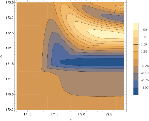


It is important to bear in mind that the source on Fig. 1 modulates how the corrections of Fig. 3 affect non-Gaussianity. So although the graph of shows a strong amplitude enhancement for , and an equally strong suppression for , the latter effect is much less significant because it peaks for , by which point is small. Because of this modulation, the biggest correction comes from the large positive phase shift at , which peaks at .


Figure 4 gives some idea of the significance of the various corrections we have introduced to the approximation of Adshead, Dvorkin, Hu and Peiris [31], but it is limited by the assumption that . The correlators Hung, Fergusson and Shellard [42] provide a more detailed comparison between any two bi-spectra and which possess the same power spectrum . They are formed from ratios of “inner products” defined as,
| (42) |
where indicates the range of the wave numbers that obey the triangle condition (), plus whatever other restrictions we wish to impose, and the multiplicative constant is irrelevant. Hung, Fergusson and Shellard use these inner products to form, respectively, shape, amplitude and total correlators,
| , | (43) | ||||
| (44) |
We evaluated all three correlators to compare our approximation (as ) with the simpler approximation (as ) of Adshead, Dvorkin, Hu and Peiris [31] over the narrow range of the greatest response. The results are,
| (45) |
Even though the equilateral triangle case shown by Figure 4 seems to roughly agree we can see there is quite a large mismatch in the amplitudes that leads to a substantial degradation of the total correlator.
4 The Square Well Model
In 1992 Starobinsky proposed a simple model in which the first slow roll parameter makes an instantaneous jump from one value to another, which permits the mode functions to be solved exactly [43]. Because the fundamental source of non-Gaussianity is a delta function for this case, one can exactly compute and derive excellent approximations for the remaining contributions [44, 45, 46]. We shall make a slight modification of this model in which returns to its original value after a short number of e-foldings ,
| (46) |
We first solve exactly for the mode functions. Next a determination is made of the parameter values for , , and to cause the scalar power spectrum of this model to agree with a numerical determination of the Step Model power spectrum of section 3.2 over the crucial range . After that is computed exactly, and then in the approximation of setting all small factors of to zero. We close by using the correlators (43-44) of Hung, Fergusson and Shellard [42] to compare this exactly solvable model with our approximation, and with the simpler approximation of Adshead, Dvorkin, Hu and Peiris [31].
For for all time then the exact mode function is,
| (47) |
For the actual parameter (46) the mode function takes the form,
| (48) | |||||
where and are,
| (49) | |||||
| (50) |
The appropriate matching conditions at and are the continuity of and of the product . The coefficients and involve the mode functions (47) and their derivatives evaluated at ,
| (51) |
The coefficients and involve the mode functions (47) and their derivatives evaluated at ,
| (52) |


From expression (50) and the small argument form of the Hankel function we infer the late time limit of the mode function,
| (53) |
Substituting this in expression (9) gives the Square Well model’s prediction for the scalar power spectrum,
| (54) |
Figure 5 compares (54) with a numerical determination of for the Step Model. There is no way to make the two results agree for all values of , however, very good concurrence over the key range of results from the following choices for the Square Well parameters,
| (55) |
The infinite sequence of oscillations (“ringing”) evident in Fig. 5 is the result of the sharp transitions in for the Square Well Model (46). For smooth transitions, such as those of the Step Model, the oscillations decay rapidly. Of course no one understands what caused features (if they are present) so it may be that the transition really is instantaneous, in which case ringing is a prominent signature that persists long after the transition. This possibility was pursued in a fascinating study by Adshead, Dvorkin, Hu and Lim [32]. However, we shall here take the view that ringing is an artifact of modelling smooth transitions as instantaneous, and we shall accordingly focus narrowly on the two e-foldings over which the Square Well model is in reasonable agreement with the Step Model.
The great advantage of the Square Well Model is that the key modulation factor of in expression (14) is a delta function,
| (56) |
where . We must also understand how to evaluate certain discontinuous factors at the jumps,
| (57) | |||||
| (58) | |||||
| (59) |
Substituting relations (56) and (57-59) into expressions (10) and (14) gives,
| (60) | |||||
where the upper and lower factors are,
| (61) | |||||
| (62) | |||||
Expressions (60-62) are exact, but somewhat opaque because they conceal certain large factors of , and because they are obscured by many other negligibly small positive powers of . There is no appreciable loss of accuracy, and a considerable simplification, by extracting the large factors of and setting the other factors of to zero. Note that this makes the Hubble parameter constant. Two ratios which involve the momenta are,
| (63) |
Applying these approximations to the mode functions (at and ) and their first derivatives gives,
| , | (64) | ||||
| , | (65) |
These approximations carry the first set of combination coefficients (51) to,
| (66) | |||||
| (67) |
Only the difference of the second set (52) matters, and it becomes,
| (68) |
With these approximations expression (14) assumes the form,
| (69) | |||||
where and the approximated factors are,
| (70) | |||||
| (71) | |||||
One can see from Figure 5 that the power spectra of the Square Well Model and the step Model agree almost perfectly over the region . This might seem to indicate that they would produce the nearly the same non-Gaussian signal, at least when restricted to the same narrow range. However, the results are disappointing when the two models are compared using the shape, amplitude and total correlators (43-44) of Hung, Fergusson and Shellard [42],
| (72) |
where was the Square Well Model and was the Step Model. The amplitudes of the two models are in much better agreement than for the comparison (45) of the Step Model with the approximation of Adshead, Dvorkin, Hu and Peiris [31]. However, the shapes disagree, which results in an even lower total correlator. Note that the problem in this case did not arise from inaccurately modeling the non-Gaussian response to a given history , but rather from the fact that different histories produce different bi-spectra, even when the power spectra are very similar.
We also compared the Square Well Model (as ) with the approximation of Adshead, Dvorkin, Hu and Peiris [31] (as ),
| (73) |
Both the shape correlator and the amplitude correlator are worse than for the comparison (45) of our approximation with that of Adshead, Dvorkin, Hu and Peiris, resulting in a much smaller total correlator.
5 Epilogue
We have examined the non-Gaussianity associated with conjectured sharp variations in the first slow roll parameter known as “features”. In section 2 we identified the crucial contribution, equation (14), which becomes significant for features. Section 3 applied an approximation for how the scalar mode functions depend analytically on [26, 34] to develop an approximation (30) for this term. Our result involves three tabulated functions of the instantaneous e-folding and the e-folding of horizon crossing :
Although generating these functions is numerically challenging, it only needs to be done over the narrow range of and associated with the feature. This is illustrated in Figure 3 which identifies the small ranges of and over which significant corrections would occur for a model of the first feature.
Our technique is more time-consuming, but also more accurate, than the approximation of Adshead, Dvorkin, Hu and Peiris [31]. When the two approximations were compared using the total correlator (44) of Hung, Fergusson and Shellard [42] the result (45) was nearly a 50% degradation of the signal, even when the comparison was restricted to a narrow range around the feature. Accurate modeling is crucial when studying features because they produce an oscillating signal, so that even small errors in the phase can significantly degrade the signal. This is especially relevant because the response to a feature is delayed to later crossing wave numbers. Unless the late time phase information is accurately modeled, trying to boost the signal by including the delayed response will actually reduce the measured signal.
In section 4 we presented a slight elaboration of a model due to Starobinsky [43] for which the crucial contribution (14) can be computed exactly, without any approximation [44, 45, 46]. In our model jumps from to and then falls back down after an interval , hence the name “Square Well Model”. Expression (60) gives the exact result for the bi-spectrum of the Square Well Model. However, taking the inessential factors of to zero produces a simpler and more transparent result (69) which is almost as accurate. A consequence of the sharp transitions is the persistence of oscillations for wave numbers which experience horizon crossing long after the transition. We regarded this as an artifact of the square well approximation, and truncated the late oscillations. For a different point of view we recommend the study of Adshead, Dvorkin, Hu and Lim [32].
Figure 4 shows that the power spectra of the Square Well Model agree with that of the Step Model over the narrow range of . However, the bi-spectra they produce are very different. We found a total shape correlator (72) of only about one third! This underlines the importance of knowing the history in addition to accurately modeling the response to it.
Acknowledgements
This work was partially supported by the European Union’s Seventh Framework Programme (FP7-REGPOT-2012-2013-1) under grant agreement number 316165; by the European Union’s Horizon 2020 Programme under grant agreement 669288-SM-GRAV-ERC-2014-ADG; by NSF grants PHY-1506513, 1806218 and 1912484; and by the UF’s Institute for Fundamental Theory.
References
- [1] V. F. Mukhanov and G. V. Chibisov, JETP Lett. 33, 532 (1981) [Pisma Zh. Eksp. Teor. Fiz. 33, 549 (1981)].
- [2] R. P. Woodard, Rept. Prog. Phys. 72, 126002 (2009) doi:10.1088/0034-4885/72/12/126002 [arXiv:0907.4238 [gr-qc]].
- [3] A. Ashoorioon, P. S. Bhupal Dev and A. Mazumdar, Mod. Phys. Lett. A 29, no. 30, 1450163 (2014) doi:10.1142/S0217732314501636 [arXiv:1211.4678 [hep-th]].
- [4] L. M. Krauss and F. Wilczek, Phys. Rev. D 89, no. 4, 047501 (2014) doi:10.1103/PhysRevD.89.047501 [arXiv:1309.5343 [hep-th]].
- [5] N. Aghanim et al. [Planck Collaboration], arXiv:1807.06209 [astro-ph.CO].
- [6] P. A. R. Ade et al. [BICEP2 and Keck Array Collaborations], Phys. Rev. Lett. 116, 031302 (2016) doi:10.1103/PhysRevLett.116.031302 [arXiv:1510.09217 [astro-ph.CO]].
- [7] N. C. Tsamis and R. P. Woodard, Annals Phys. 267, 145 (1998) doi:10.1006/aphy.1998.5816 [hep-ph/9712331].
- [8] T. D. Saini, S. Raychaudhury, V. Sahni and A. A. Starobinsky, Phys. Rev. Lett. 85, 1162 (2000) doi:10.1103/PhysRevLett.85.1162 [astro-ph/9910231].
- [9] T. Padmanabhan, Phys. Rev. D 66, 021301 (2002) doi:10.1103/PhysRevD.66.021301 [hep-th/0204150].
- [10] S. Nojiri and S. D. Odintsov, Gen. Rel. Grav. 38, 1285 (2006) doi:10.1007/s10714-006-0301-6 [hep-th/0506212].
- [11] R. P. Woodard, Lect. Notes Phys. 720, 403 (2007) doi:10.1007/978-3-540-71013-4_14 [astro-ph/0601672].
- [12] Z. K. Guo, N. Ohta and Y. Z. Zhang, Mod. Phys. Lett. A 22, 883 (2007) doi:10.1142/S0217732307022839 [astro-ph/0603109].
- [13] A. Ijjas, P. J. Steinhardt and A. Loeb, Phys. Lett. B 723, 261 (2013) doi:10.1016/j.physletb.2013.05.023 [arXiv:1304.2785 [astro-ph.CO]].
- [14] A. H. Guth, D. I. Kaiser and Y. Nomura, Phys. Lett. B 733, 112 (2014) doi:10.1016/j.physletb.2014.03.020 [arXiv:1312.7619 [astro-ph.CO]].
- [15] A. Linde, doi:10.1093/acprof:oso/9780198728856.003.0006 arXiv:1402.0526 [hep-th].
- [16] A. Ijjas, P. J. Steinhardt and A. Loeb, Phys. Lett. B 736, 142 (2014) doi:10.1016/j.physletb.2014.07.012 [arXiv:1402.6980 [astro-ph.CO]].
- [17] P. A. R. Ade et al. [Planck Collaboration], Astron. Astrophys. 594, A20 (2016) doi:10.1051/0004-6361/201525898 [arXiv:1502.02114 [astro-ph.CO]].
- [18] J. Torrado, B. Hu and A. Achucarro, Phys. Rev. D 96, no. 8, 083515 (2017) doi:10.1103/PhysRevD.96.083515 [arXiv:1611.10350 [astro-ph.CO]].
- [19] J. Martin and C. Ringeval, JCAP 0608, 009 (2006) doi:10.1088/1475-7516/2006/08/009 [astro-ph/0605367].
- [20] L. Covi, J. Hamann, A. Melchiorri, A. Slosar and I. Sorbera, Phys. Rev. D 74, 083509 (2006) doi:10.1103/PhysRevD.74.083509 [astro-ph/0606452].
- [21] J. Hamann, L. Covi, A. Melchiorri and A. Slosar, Phys. Rev. D 76, 023503 (2007) doi:10.1103/PhysRevD.76.023503 [astro-ph/0701380].
- [22] D. K. Hazra, A. Shafieloo, G. F. Smoot and A. A. Starobinsky, JCAP 1408 (2014) 048 doi:10.1088/1475-7516/2014/08/048 [arXiv:1405.2012 [astro-ph.CO]].
- [23] D. K. Hazra, A. Shafieloo, G. F. Smoot and A. A. Starobinsky, JCAP 1609, no. 09, 009 (2016) doi:10.1088/1475-7516/2016/09/009 [arXiv:1605.02106 [astro-ph.CO]].
- [24] A. Achúcarro, J. O. Gong, G. A. Palma and S. P. Patil, Phys. Rev. D 87, no. 12, 121301 (2013) doi:10.1103/PhysRevD.87.121301 [arXiv:1211.5619 [astro-ph.CO]].
- [25] D. J. Brooker, N. C. Tsamis and R. P. Woodard, Phys. Lett. B 773, 225 (2017) doi:10.1016/j.physletb.2017.08.027 [arXiv:1603.06399 [astro-ph.CO]].
- [26] D. J. Brooker, N. C. Tsamis and R. P. Woodard, Phys. Rev. D 96, no. 10, 103531 (2017) doi:10.1103/PhysRevD.96.103531 [arXiv:1708.03253 [gr-qc]].
- [27] J. M. Maldacena, JHEP 0305, 013 (2003) doi:10.1088/1126-6708/2003/05/013 [astro-ph/0210603].
- [28] J. R. Fergusson and E. P. S. Shellard, Phys. Rev. D 76, 083523 (2007) doi:10.1103/PhysRevD.76.083523 [astro-ph/0612713].
- [29] J. R. Fergusson and E. P. S. Shellard, Phys. Rev. D 80, 043510 (2009) doi:10.1103/PhysRevD.80.043510 [arXiv:0812.3413 [astro-ph]].
- [30] P. A. R. Ade et al. [Planck Collaboration], Astron. Astrophys. 594, A17 (2016) doi:10.1051/0004-6361/201525836 [arXiv:1502.01592 [astro-ph.CO]].
- [31] P. Adshead, W. Hu, C. Dvorkin and H. V. Peiris, Phys. Rev. D 84, 043519 (2011) doi:10.1103/PhysRevD.84.043519 [arXiv:1102.3435 [astro-ph.CO]].
- [32] P. Adshead, C. Dvorkin, W. Hu and E. A. Lim, Phys. Rev. D 85, 023531 (2012) doi:10.1103/PhysRevD.85.023531 [arXiv:1110.3050 [astro-ph.CO]].
- [33] D. K. Hazra, L. Sriramkumar and J. Martin, JCAP 1305, 026 (2013) doi:10.1088/1475-7516/2013/05/026 [arXiv:1201.0926 [astro-ph.CO]].
- [34] D. J. Brooker, N. C. Tsamis and R. P. Woodard, JCAP 1804, no. 04, 003 (2018) doi:10.1088/1475-7516/2018/04/003 [arXiv:1712.03462 [gr-qc]].
- [35] A. R. Liddle, P. Parsons and J. D. Barrow, Phys. Rev. D 50, 7222 (1994) doi:10.1103/PhysRevD.50.7222 [astro-ph/9408015].
- [36] V. F. Mukhanov, H. A. Feldman and R. H. Brandenberger, Phys. Rept. 215, 203 (1992). doi:10.1016/0370-1573(92)90044-Z
- [37] A. R. Liddle and D. H. Lyth, Phys. Rept. 231, 1 (1993) doi:10.1016/0370-1573(93)90114-S [astro-ph/9303019].
- [38] D. S. Salopek, J. R. Bond and J. M. Bardeen, Phys. Rev. D 40, 1753 (1989). doi:10.1103/PhysRevD.40.1753
- [39] M. G. Romania, N. C. Tsamis and R. P. Woodard, JCAP 1208, 029 (2012) doi:10.1088/1475-7516/2012/08/029 [arXiv:1207.3227 [astro-ph.CO]].
- [40] J. A. Adams, B. Cresswell and R. Easther, Phys. Rev. D 64, 123514 (2001) doi:10.1103/PhysRevD.64.123514 [astro-ph/0102236].
- [41] M. J. Mortonson, C. Dvorkin, H. V. Peiris and W. Hu, Phys. Rev. D 79, 103519 (2009) doi:10.1103/PhysRevD.79.103519 [arXiv:0903.4920 [astro-ph.CO]].
- [42] J. Hung, J. R. Fergusson and E. P. S. Shellard, arXiv:1902.01830 [astro-ph.CO].
- [43] A. A. Starobinsky, JETP Lett. 55, 489 (1992) [Pisma Zh. Eksp. Teor. Fiz. 55, 477 (1992)].
- [44] F. Arroja, A. E. Romano and M. Sasaki, Phys. Rev. D 84, 123503 (2011) doi:10.1103/PhysRevD.84.123503 [arXiv:1106.5384 [astro-ph.CO]].
- [45] J. Martin and L. Sriramkumar, JCAP 1201, 008 (2012) doi:10.1088/1475-7516/2012/01/008 [arXiv:1109.5838 [astro-ph.CO]].
- [46] F. Arroja and M. Sasaki, JCAP 1208, 012 (2012) doi:10.1088/1475-7516/2012/08/012 [arXiv:1204.6489 [astro-ph.CO]].