Order reduction methods for solving large-scale differential matrix Riccati equations Thanks: This version dated December 20, 2019
Abstract
We consider the numerical solution of large-scale symmetric differential matrix Riccati equations. Under certain hypotheses on the data, reduced order methods have recently arisen as a promising class of solution strategies, by forming low-rank approximations to the sought after solution at selected timesteps. We show that great computational and memory savings are obtained by a reduction process onto rational Krylov subspaces, as opposed to current approaches. By specifically addressing the solution of the reduced differential equation and reliable stopping criteria, we are able to obtain accurate final approximations at low memory and computational requirements. This is obtained by employing a two-phase strategy that separately enhances the accuracy of the algebraic approximation and the time integration. The new method allows us to numerically solve much larger problems than in the current literature. Numerical experiments on benchmark problems illustrate the effectiveness of the procedure with respect to existing solvers.
keywords
Differential Matrix Riccati, Rational Krylov, Extended Krylov, Linear Quadratic Regulator, Low-rank, BDF1 Introduction
We consider the solution of the continuous-time differential matrix Riccati equation (DRE in short) of the form
| (1) |
in the unknown matrix , where and . Here, , , and are time invariant, and . The matrix is assumed to be large, sparse and nonsingular, whereas , and have full rank. In particular, we consider low-rank DREs, where both matrices and have very low rank compared to . Even though the matrix is sparse, the solution is typically dense and impossible to store when is large. Under the considered hypotheses, numerical evidence seems to indicate that usually has rapidly decaying singular values, hence a low-rank approximation to may be considered, see e.g., [48]. For completeness, we also refer the reader to [21, 20] for results on the existence of low-rank solutions for the algebraic Sylvester and Lyapunov (linear) equations.
The DRE plays a fundamental role in optimal control theory, filter design theory, model reduction problems, as well as in differential games [2, 7, 11, 13, 38]. Equations of the form eq. 1 are crucial in the numerical treatment of the linear quadratic regulator (LQR) problem [2, 13, 29]: given the state equation
| (2) |
consider the finite horizon case, where the finite time cost integral has the form
| (3) |
The matrix is assumed to be symmetric and nonnegative definite. Assuming that the pair is stabilizable and the pair is detectable, the optimal input , minimizing eq. 3, can be determined as , and the optimal trajectory is subject to . The matrix is the solution to the DRE
| (4) |
Using a common practice, we can transform eq. 4 into the initial value problem eq. 1 via the change of variables .
Under certain assumptions, the exact solution of eq. 1 can be expressed in integral form as (see e.g., [28, Theorem 8])
| (5) |
so that when the DRE reaches a steady state solution satisfying the algebraic Riccati equation (ARE)
| (6) |
In the framework of differential equations, the DRE is characterized by both fast and slow varying modes, hence it is classified as a stiff ordinary differential equation (ODE). The stiffness and the nonlinearity of the DRE are responsible for the difficulties in its numerical solution even on a small scale (). Several stiff integrators have been investigated, including the matrix generalizations of implicit ODE solvers [15, 12], linearization methods [14] and more recently matrix versions of splitting methods [35, 46, 47]. These methods are feasible on a small scale but fail to be efficient when is large. In [41], iterative methods are implemented within the matrix generalization of standard implicit methods allowing for the computation of an approximate solution to the DRE when . These algorithms require the solution of a large algebraic Riccati equation at each timestep, which again raises big concerns as of storage and computational efforts.
A promising idea is to rely on a model order reduction strategy typically used in linear and nonlinear dynamical systems. In this setting, the original system is replaced with
| (7) |
where and are projections and restrictions of the original matrices onto a subspace of small dimension. The differential Riccati equation associated with this reduced order problem is solved, yielding an optimal corresponding cost function. This strategy allows for a natural low-rank approximation to the sought after DRE solution , obtained by interpolating the reduced order solution at selected time instances. One main feature is that a single space is used for all time snapshots, so that the approximate solutions can be kept in factored form with few memory allocations. We refer the reader to, e.g., [4] for a general presentation of algebraic reduction methods for linear dynamical systems, and to [43] for a detailed discussion motivating the reduction approach in the context of the algebraic Riccati equation.
A key ingredient for the success of the reduction methodology is the choice of the approximation space onto which the algebraic reduction is performed; [4] presents a comprehensive description of various space selections in the dynamical system setting. Following strategies already successfully adopted for the algebraic Riccati equations, the authors of [27] and [23] have independently used polynomial and extended Krylov subspaces as approximation space, respectively, in the differential setting. A major characteristic of these spaces is that their dimension can be expanded iteratively, so that if the determined approximate solution is not sufficiently accurate, the Krylov space can be enlarged and the process continued. Several questions remain open in the methods proposed in [27],[23]. On the one hand, it is well known that polynomial Krylov subspaces require a very large dimension to satisfactorily solve real application problems, thus destroying the reduction advantages. On the other hand, the multiple timestepping proposed in the method in [23] only provides an accurate approximation at , except when . For of low rank, memory requirements of the extended method grow significantly. These problems can be satisfactorily solved by using a general rational Krylov subspace, which is shown in various applications to be able to supply good spectral information on the involved matrices with much smaller dimensions than the polynomial and extended versions. Such gain has been experimentally reported in the literature in the solution of the algebraic Riccati equation. We show that great computational and memory savings can be obtained when projecting onto the fully rational Krylov subspace, and that with an appropriate implementation the extended Krylov subspace may also be competitive with certain data.
A related issue that has somehow been overlooked in the available literature is the expected final accuracy and thus the stopping criterion. Time dependence of the DRE makes the reduced problem trickier to handle than in the purely algebraic case; in particular, two intertwined issues arise: i) The accuracy of the approximate solution may vary considerably within the time interval ; ii) Throughout the reduction process the reduced ODE cannot be solved with high accuracy and, quite the opposite, low-order methods should be used to make the overall cost feasible. We analyze these difficulties in detail, and by exploiting the inherent structure of the reduced order model, we derive a two-phase strategy that first focuses on the reduction and then on the integration, in a way that is efficient for memory and CPU time usage, but also in terms of final expected accuracy.
We also discuss several algebraic properties of the approximate solution and its relation both with the solution for , and with the steady state solution . These results continue a matrix analysis started in [27], where positivity and monotonicity properties of the approximate solution obtained by certain reduction methods are explored.
The paper is organized as follows. In section 2 we introduce reduction methods and discuss the use of Krylov subspace based strategies. Matrix-oriented BDF methods are recalled for the solution of the projected problem in section 3. In section 4 we devise a stopping criterion for the order reduction methods and illustrate its key role in the implementation. Section 5 is devoted to the analysis of matrix properties of the solution, as well as the reduced model, from a control theory perspective. Several numerical experiments are reported in section 6, where the new methods are also compared with state-of-the-art procedures. Our conclusions are discussed in section 7. Finally, in appendix A and appendix B we review some properties of the extended and rational Krylov subspaces.
Notation and definitions. Throughout the paper, the matrix will denote the identity matrix. In terms of norms, refers to any induced matrix norm, where in particular the Frobenius norm is denoted by . A matrix is stable (sometimes also called Hurwitz) if all its eigenvalues are contained in the left half open complex plane. A linear dynamical system, is called dissipative if the real matrix has its field of values contained in the left half open complex plane.
All reported experiments were performed using MATLAB 9.4 (R2018b) ([33]) on a MacBook Pro with 8-GB memory and a 2.3-GHz Intel core i5 processor.
2 Order reduction with Krylov-based subspaces
In this section, we review Krylov-based order reduction methods and show how they are applied to the DRE. Krylov subspaces that have been explored in the past years have the form
where is a tall matrix associated with the given problem. In the rational subspace, is a set of properly chosen real or complex shifts, whose computation can be performed a priori or dynamically during the generation of the subspace; we refer the reader to [44, 18] for more complete descriptions.
Krylov-based projection methods (in short generically denoted as ) were first applied to ARE’s in [25] (polynomial spaces) and later improved in [24] (extended space) and [45] (rational spaces). The two rational spaces prove to be far superior to the polynomial Krylov space in most reduction strategies where they are applied in the literature, as long as solving linear systems at each iteration is feasible. The differential Riccati equation has been attacked in [23] with the extended space, and in [27] with the polynomial space; here we close the gap, as far as Krylov subspaces are concerned. In addition, we address several implementation issues to make the final method computationally reliable and, to the best of our knowledge, a great competitor among the available methods for large-scale DRE problems.
While for the algebraic Riccati equation , in the differential context the starting matrix for generating these spaces is given by , where . Both matrices and play a crucial role in the closed-form DRE solution matrix and are thus included to generate the projection space. The idea of reduction methods is to first project the large DRE onto the smaller subspace , then solve the projected equation, and finally expand the solution back to the original space.
Let the columns of span the considered Krylov subspace. Then the following Arnoldi-type relation holds,
| (8) |
where the actual values of and depend on the chosen subspace. Moreover, setting we have that , which shows that Krylov subspaces are nested, that is , resulting in a dimension increase after each iteration. Matrix relations leading to eq. 8 for the extended and rational Krylov subspaces are recalled in appendix A.
Assume that has orthonormal columns. Following similar reduction methods in the dynamical system contexts, see, e.g., [4], the reduction process consists of first projecting and restricting the original data onto the approximation space as
Then the following low order differential Riccati equation needs to be solved,
| (9) |
for . This low-dimensional DRE admits a unique solution for , see e.g., [28]. Restrictions on the data to allow for positive, stabilizing solutions are discussed in more detail in section 5.1. An approximation to the sought after solution is then written as
| (10) |
We stress that is never explicitly computed, but always referred to via the matrix and the set of matrices at given time instances. In fact, the matrices may also be numerically low rank, so that at the end of the whole process a further reduction can be performed by truncating the eigendecomposition of for each .
Remark 1.
The approach we have derived is solely based on the order reduction of the dynamical system (2). Nonetheless, and with some abuse of notation, the reduced DRE could have been formally obtained by means of a Galerkin condition on the differential equation. For let
be the residual matrix for . The matrix is thus determined by imposing that the residual satisfies the following Galerkin condition
| (11) |
that is, in a matrix sense, so that the residual is forced to belong to a smaller and smaller subspace as grows. Substituting into the residual matrix, the application of the Galerkin condition results in the projected system
which corresponds to (9). This is rigorous as long as holds.
It is crucial to realize that, as opposed to some available methods in the literature (such as, for instance, [41],[47] and the time-invariant algorithms in [30]), the approximation space is independent of the time stepping, that is a single space range is used for all time steps. This provides enormous memory savings whenever the approximate solution is required at different time instances in . Theoretical motivation for keeping the approximation space independent of the time-stepping is contained in [5], where it is shown that the solution of the DRE lives in an invariant Krylov-subspace11 1 We also refer the reader to the recent manuscript [6], which appeared on-line briefly before the first round of our revision..
The class of numerical methods we used for solving the reduced DRE is described in the next section. In the rest of this paper, we specialize the generic derivation above to the extended and rational Krylov subspaces, which greatly outperformed polynomial spaces both in terms of CPU time and memory requirements. More information on these spaces and their properties are given in appendix A; in particular, we discuss the generation of a real rational Krylov basis in the presence of non-real shifts.
3 BDF methods for the DRE
The numerical solution of the small-scale DRE is a well-studied topic, see, e.g., [34, 14, 35, 46]. Among the explored methods are matrix generalizations of the BDF methods [34, 15], which are computationally appealing only for small problems. Due to the reduction strength of rational Krylov subspaces, we expect the reduced DRE in eq. 9 to be small enough to allow for efficient use of matrix-based BDF methods, which we are going to summarize next. For simplicity of exposition, in the rest of this section we omit the subscript in , and denote . If we define
| (12) |
the approximation of is given by the implicit relation
| (13) |
where is the stepsize and the respective ’s and are the coefficients of the -step BDF method for and are given below.
| 1 | 1 | 1 | ||
|---|---|---|---|---|
| 2 | ||||
| 3 |
Substituting eq. 12 into eq. 13 results in the following nonlinear matrix equation
which can be reformulated as the following continuous-time ARE
| (14) |
The coefficient matrices are given by
The Riccati equation eq. 14 can be solved using “direct” methods; see, e.g., [9]. In our experiments we used the MATLAB solver care from the control systems toolbox. A brief sketch of the -step BDF method is reported in algorithm 1; other approaches are discussed, e.g., in [34, 30].
We conclude the section by depicting the typical convergence behavior of the BDF methods in our context. We consider an example from [35], where the matrix stems from the spatial finite difference discretization of the following advection-diffusion equation
on with homogeneous Dirichlet boundary conditions. The choices of and are given binomially as described in [35]. The initial condition is taken to be the zero matrix, that is . We compare the obtained solution with a “reference” numerical solution computed by an accurate but expensive method (the MATLAB function ode23s in our experiments), so that is kept small, . The convergence behavior for and timesteps, with is displayed in fig. 1. The left plot shows the error as a function of , for different values of . The right plot shows the evolution of the (1,1) component of the solution throughout the time span for the most accurate choice of BDF method, compared with that of the reference solution.


These plots illustrate that we cannot expect an overall high accuracy of the projection method as long as the reduced differential equation is not solved with sufficiently good accuracy. The importance of this is discussed in more detail in the following section.
4 Stopping criterion and the complete algorithm
To complete the reduction algorithm of section 2, we need to introduce a stopping criterion. We found that it is crucial to take into account the accuracy of the numerical method employed to solve the reduced DRE, as discussed in section 3.
To derive our stopping criterion we were inspired by those in [27, 23], however, we made some important modifications. In both cited references, the authors assume that the inner problem eq. 9 is solved exactly, which is not true in general. We thus consider that the numerical method solves the reduced problem with residual matrix , so that the final DRE residual can be split into two components.
Proposition 2.
Proof.
The expression for emphasizes that at each iteration the matrix is the exact solution of
Hence, as long as is not very small, the increase of aims at more and more accurately approximating a “nearby” differential problem to the truly projected one, with a term that varies with . Hence, is an approximation not to , but to the solution of a differential problem with an additional term whose projection onto the space is .
Proposition 2 also implies that we cannot expect an overall small residual norm if either of the two partial residual norms , is not small. In particular, we observe that the two residuals can be made small independently. Therefore we propose the following practical strategy:
- (i)
Run the algorithm as presented, with a low-order cheap ODE inner solver (i.e., BDF(1, ) with relatively small) and use in the stopping criterion;
- (ii)
Once completed step (i) after iterations, use the matrices and to refine the ODE inner solution by using a higher-order ODE solver for the projected system.
The final matrix obtained in step (ii) will provide a more accurate solution matrix than what would have been obtained at the end of step (i). We emphasize that any ODE method for small and medium scale DREs could be used at steps (i) and (ii). Our choice of BDF(1, is due to its good trade-off between accuracy and computational effort; other approaches could be considered.
To complete the description of the stopping criterion, we recall that depends on , so that we need to estimate the integral over the whole time interval by means of a quadrature formula, that is
| (17) |
where the interval has been divided into intervals with nodes .
The overall algorithm22 2 A Matlab implementation of both algorithms will be made available upon publication of this work. based on the rational Krylov subspace method is reported in algorithm 2, while the algorithm based on the extended method is postponed to appendix B. Several implementation issues of algorithm 2 are also described in appendix A, such as the use of a real basis in case of complex shifts in the basis construction.
5 Stability analysis and error bounds
In this section, we provide a few results on the spectral and convergence properties of the obtained approximate solution We first inspect some properties of the asymptotic matrix solution, which solves the algebraic Riccati equation. Then we propose a bound for the error matrix, in an appropriate functional norm.
5.1 Properties of the (steady state) algebraic Riccati equation
Properties associated with the algebraic Riccati equation – as asymptotic solution to the DRE – are well known in linear quadratic optimal control, see, e.g., [29, 13]. In particular, classical uniqueness and stabilization properties of the solution (see, e.g., [13, Lemma 12.7.2]), can directly be extended to the reduced DRE eq. 9.
Corollary 3.
Let be stabilizable and detectable system. Let be the solution of eq. 9 at time and let . Then is the unique symmetric nonnegative definite solution and the only stabilizing solution to the (reduced) algebraic Riccati equation
| (18) |
Moreover, if the pair is observable, is strictly positive definite.
We notice that the stabilizability and detectability properties of are not necessarily implied by those on . Nevertheless, it is shown in [43] that if there exists a feedback matrix , such that the linear dynamical system is dissipative, then the pair is stabilizable. A similar result can be formulated for the detectability of , since by duality reasoning, is detectable if is stabilizable. The question regarding the existence of such a feedback matrix, with respect to and ( and ), is addressed in [22].
With these results, we can relate the asymptotic solution of the original and projected problems. Let and respectively be approximate solutions to eqs. 1 and 6 by a projection onto . If there exist matrices and such that the systems and are dissipative, then
| (19) |
that is, is the steady state solution of when projected onto the same basis.
Under the hypotheses that is a stabilizable and detectable system, there exists a unique non-negative and stabilizing solution to eq. 6 (see, e.g., [28, Theorem 5]). In [43] a bound was derived for the error in terms of the matrix residual norm. Here we complete the argument by stating that in exact arithmetic and if the whole space can be spanned, the obtained approximate solution equals .
Proposition 4.
Suppose is stabilizable and detectable. Assume it is possible to determine such that , and let be the obtained approximate solution of eq. 6 after iterations. Then, .
Proof.
Since is square and orthogonal the projected ARE is given by
From stabilizable and detectable it follows that is also stabilizable and detectable, so that and stabilizing. Multiplying by (by ) from the left (right), we obtain that is, is a solution to the original ARE. Since is the unique nonnegative definite solution, it must be .
5.2 Error bound for the differential Riccati equation
In this section we derive a bound for the maximum error obtained by the reduction process, in terms of the residual
| (20) |
Note that is the residual matrix with respect to the exact solution of the reduced differential problem, that is, it also includes the discretization error. A similar bound on the error has been derived for the nonsymmetric DRE in [3], which used matrix perturbation techniques from [26].
Proposition 5.
For let and assume that is stable for all . Denote
where is the state-transition matrix satisfying .
If , then
where for any continuous matrix function .
Proof.
By subtracting eq. 20 from eq. 1 and manipulating terms we obtain
with . Therefore, by the variation of constants formula (see, e.g., [28])
Taking norms yields
so that Solving this quadratic inequality yields
The result follows from multiplying and dividing by and noticing that at the denominator this quantity can be bounded from below by 1.
We conclude with a remark on the intuitive fact that if the approximation space spans the whole space, the obtained solution by projection necessarily coincides with the sought after solution of the DRE.
Remark 6.
If it is possible to determine such that , then the approximate solution coincides with for all . Indeed, let us write , where is square and orthogonal. The reduced DRE is given by
with . Multiplying by (by ) from the left (right), we obtain
hence, is a solution of eq. 1. Since is the unique nonnegative definite solution of eq. 1 for any (see, e.g., [28]), then for .
6 Numerical experiments
In this section we report on our numerical experience with the developed techniques. We consider two artificial symmetric and nonsymmetric model problems, as well as three (of which two are nonsymmetric) standard benchmark problems. Information about the considered data is contained in table 1. For the first two datasets displayed in table 1, the matrix stems from the finite difference discretization with homogenous Dirichlet boundary conditions on the unit square and unit cube, respectively. The first matrix (sym2d) comes from the finite difference discretization of the two-dimensional Laplace operator in the unit square with homogeneous boundary conditions, while the second matrix (nsym3d) stems from the finite difference discretization of the three-dimensional differential operator
in the unit cube, with homogeneous boundary conditions. For both datasets, the matrices and are selected randomly with normally distributed entries. The realizations of the random matrices are fixed for both examples using the MATLAB command rng: for and we use rng(7), rng(2) and rng(3), respectively. The following two datasets ( chip and flow) are taken from [1], and all coefficient matrices (, , and ) are contained in the datasets, which stem from the dynamical system
Since is diagonal and nonsingular, it is incorporated as , while and are updated accordingly to form and .
The final considered dataset (rail) stems from a semi-discretized heat transfer problem for optimal cooling of steel profiles33 3 Data available at http://modelreduction.org/index.php/Steel_Profile [8]. We consider the largest of the four available discretizations (file rail_79841_c60 containing and ) with . The symmetric and positive definite mass matrix has a sparsity pattern very similar to . Both matrices are therefore reordered by the same approximate minimum degree (rksm-dre) or reverse Cuthill-McKee (eksm-dre) permutation to limit fill-in. The state-space transformation is done using the Cholesky factorization of . More precisely, let with lower triangular, and consider the transformed state . Then
with , and . These matrices are never explicitly formed, rather they are commonly applied implicitly by solves with the factor at each iteration; see, e.g., [18, 42].
The initial low-rank factors are selected as the zero vector for flow, for chip and for rail, where is a vector with entries in . Other sufficiently general choices were tried during our numerical investigation however results did not significantly differ from the ones we report.
| Name | // | ||||||
|---|---|---|---|---|---|---|---|
| sym2d | |||||||
| nsym3d | 6/1/3 | ||||||
| Name | // | ||||||
| chip | 5/1/1 | ||||||
| flow | 5/1/1 | ||||||
| rail | 7/6/1 |
Performance of the projection methods. We first investigate the convergence behavior of the outer solver. The quantity we monitor in our stopping criterion is the backward error in an integral norm given by
| (21) |
with as in eq. 17 and
The integrals are approximated by a quadrature formula in a similar fashion to eq. 17, and we note that can be cheaply computed by using the Arnoldi-type relation.
For all datasets, the stopping tolerance was chosen as . For the first four datasets, and bdf(1,10) is used as inner solver. For rail, (see e.g., [8] for further details about the setting) and bdf(1,45) is used as inner solver. figs. 2 to 6 display the convergence of the rational Krylov subspace method (algorithm 2, rksm-dre) and of the extended Krylov subspace method (algorithm 3, eksm-dre). The left plots report the history of the backward error as the approximation space dimension increases, while the right plots display the same history versus the total computational time (in seconds) as the iterations proceed. We notice that the cost of the refinement step is not taken into account in these first tests.


For the dataset sym2d, the large algebraic linear system in rksm-dre was iteratively solved by implementing a block conjugate gradient algorithm, with an inner tolerance of , preconditioned with an incomplete Cholesky factorization with drop tolerance . For all other datasets, the MATLAB built-in backslash operator was used. For eksm-dre the coefficient matrix used to generate the Krylov space remains constant, hence a sparse reordered Cholesky (for sym2d and rail) or LU (for all other datasets) factorization was performed once and for all at the start of the algorithm. Therefore, only sparse triangular solves are required at each iteration. Clearly, the cost of the initial factorization depends on the size and density of the coefficient matrix. These two cost stages are particularly noticeable in the right plots of fig. 3 and fig. 4, where the eksm-dre curve starts towards the right of the plot, while the rest of the computation throughout the iterations is significantly faster.
In the implementation of rksm-dre it is possible to decide a priori whether to use only real or generically complex shifts. Our experiments showed that complex shifts were unnecessary for sym2d and nsym3d and, in fact, slowed down convergence when used. On the other hand, the use of general complex shifts proved to be crucial for the efficient convergence of rksm-dre for chip and flow. For the symmetric data in rail no complex shifts were used. We mention in passing that both algorithms are implemented so that the inner solves of eq. 9 and the residual computations are performed at each iteration; for more demanding data we would advise a user to perform these computations only periodically to save on computational time.
Comparing performance, we observe that the two algorithms have alternating leadership in terms of computational time, but that rksm-dre almost consistently requires half the space dimension of eksm-dre. This is expected as the space dimension of eksm-dre increases with twice the number of columns per iteration, in comparison to rksm-dre. This observation is crucial at the refinement step, where it could be considerably more expensive to accurately integrate a DRE of dimension in comparison to a DRE with approximately half the dimension.
To have a clearer picture of how the various steps influence the performance of the methods, table 2 depicts the overall computational time for the system solves, the orthogonalization steps and the integration of the reduced systems for each algorithm. For eksm-dre the CPU time required for the Cholesky and factorizations are included in the solving time, but indicated in brackets as well. It is particularly interesting to notice the small percentage of time required by rksm-dre in comparison to eksm-dre for integrating the reduced system, confirming the comment made in the previous paragraph.
| System | Orthogonalisation | Integration | ||
| Data | Method | solves (s) | steps (s) | steps (s) |
| sym2d | rksm-dre | 6.1 | 6.9 | 0.4 |
| eksm-dre | 8.6 (2.7) | 12.1 | 1.3 | |
| nsym3d | rksm-dre | 38.3 | 0.9 | 0.8 |
| eksm-dre | 48.6 (43.5) | 1.6 | 4.0 |
Comparisons with other BDF based methods. We compare the two projection methods rksm-dre and eksm-dre with low-rank methods that have been developed following different strategies. The package m.e.s.s. [41], for instance, can solve Lyapunov and Riccati equations, and perform model reduction of systems in state space and structured differential algebraic form, with time-variant and time-invariant data. For our purposes, the solvers in m.e.s.s. first discretize the time interval, and then solve the algebraic Riccati equation resulting from the ODE solver at each time step. Therefore, the approximation strategy employed at each time iteration to solve the algebraic problem is completely independent, and the obtained low-rank numerical solution needs to be stored separately. More precisely, if timesteps are performed, the procedure requires solving at least AREs of large dimensions, delivering the corresponding low-rank approximate solutions. Moreover, the rank of the constant term in the ARE increases with the time step, due to the way the ODE solver is structured, further increasing the complexity of the ARE numerical treatment. In our experiments with m.e.s.s. we only requested the approximate solution at the final stage. If the whole approximate solution matrix is requested at different time instances, the memory requirements will grow linearly with that. The overall strategy appears to be memory and computational time consuming, therefore we considered datasets of reduced size for our comparisons, as displayed in table 3. The considered timespans were left unchanged.
| Name | // | ||||||
|---|---|---|---|---|---|---|---|
| sym2d | 5/1/1 | ||||||
| nsym3d | 6/1/3 | ||||||
| Name | // | ||||||
| flow | 5/1/1 | ||||||
| rail | 7/6/1 |
Our experimental results are displayed in tables 4 to 7; we remark that now also the refinement cost is taken into account in the projection methods. In all tables, the code bdf() refers to the BDF method implemented in the refinement procedure of the reduction methods and in the time discretization procedure of m.e.s.s.
| # -long | Min/Max | Reduction | Refine | Tot CPU | |
|---|---|---|---|---|---|
| Method | Vecs | rank | phase(s) | phase(s) | time(s) |
| rksm-dre | 66 | 23/43 | 1.5 | 0.19 | 1.7 |
| eksm-dre | 144 | 23/43 | 1.9 | 2.8 | 4.7 |
| m.e.s.s.-bdf(1,10) | 988 | 58/75 | 319.9 | ||
| m.e.s.s.-bdf(2,100) | 1032 | 58/86 | 4005.4 |
The tables show the storage requirements in terms of -length vectors, the minimum and maximum approximate solution rank (with a truncation tolerance for the projection methods) within the set of solutions, the CPU time break out of projection and refinement phases for the two projected methods, and finally the total CPU time. The stopping tolerance for all algebraic methods – that is the two projection methods and the Newton–Kleinmann-type method used in m.e.s.s. to solve each ARE – is set to .
In the m.e.s.s. software the user can either select a stopping tolerance (to be used for all solvers within the Newton–Kleinmann strategy) or a maximum number of iterations. We have experimented with both cases, where the maximum number of iterations was detected (a-posteriori) as the maximum number of iterations required within m.e.s.s to reach the tolerance of . It was observed that, in the majority of cases, avoiding the residual computation may, in fact, slow down the computational procedure. This is due to the possibility of performing several unnecessary iterations at some timesteps after the desired accuracy has in fact been reached. We therefore only report the results of the more realistic, reliable case where a stopping tolerance is selected beforehand. Galerkin acceleration is used to boost the performance of Newton–Kleinmann.
| # -long | Min/Max | Reduction | Refine | Tot CPU | |
|---|---|---|---|---|---|
| Method | Vecs | rank | phase(s) | phase(s) | time(s) |
| rksm-dre | 108 | 36/66 | 4.5 | 4.6 | 9.1 |
| eksm-dre | 196 | 36/66 | 2.8 | 5.7 | 8.5 |
| m.e.s.s.-bdf(1,10) | 1116 | 71/90 | 431.0 | ||
| m.e.s.s.-bdf(2,100) | 1152 | 67/94 | 4965.0 |
All numbers in the tables illustrate the large computational costs of m.e.s.s., as expected by the strategy “first time-discretize, then solve”, whereas both projection methods require just a few seconds of CPU in most cases.
The storage requirements of both reduction methods is independent of the number of timesteps where the solution is required. This is due to the fact that only a few -long basis vectors need to be generated and stored, while only the reduced problem solution changes at the timesteps . The memory requirements of m.e.s.s. are measured as the dimensions of the low-rank factor returned by the Newton-Kleinmann procedure, before column compression, at the final timestep. The dimension decreases significantly with the column compression. In our experiments we only stored the approximate solution at the last time step, however memory will be correspondingly higher if the whole approximation matrix is required at more instances (memory will thus grow linearly with the number of time instances to be monitored).
Between the two projection methods, we observe that the extended space yields a significantly larger basis than the actual approximate solution rank it produces. This means that the approximate solution belongs to a much smaller space than the one constructed by eksm-dre. This is far less so with rksm-dre. The different behavior confirms what has been already observed for the two methods in the ARE case [45].
| # -long | Min/Max | Reduction | Refine | Tot CPU | |
|---|---|---|---|---|---|
| Method | Vecs | rank | phase(s) | phase(s) | time(s) |
| rksm-dre | 186 | 95/100 | 12 | 4.6 | 16.6 |
| eksm-dre | 372 | 95/100 | 30.8 | 23.7 | 54.5 |
| m.e.s.s.-bdf(1,10) | 1280 | 87/106 | 431.7 |
| # -long | Min/Max | Reduction | Refine | Tot CPU | |
|---|---|---|---|---|---|
| Method | Vecs | rank | phase(s) | phase(s) | time(s) |
| rksm-dre | 168 | 153/160 | 6.4 | 3.3 | 9.7 |
| eksm-dre | 462 | 153/160 | 39.2 | 5.7 | 44.9 |
| m.e.s.s.-bdf(1,10) | 6345 | 151/158 | 705.3 | ||
| m.e.s.s.-bdf(2,100) | 4023 | 124/158 | 3396.5 |
Comparisons with splitting methods. We next compare rksm-dre with the fourth order additive splitting method (split-add4()) developed in [47]. The method is based on splitting the DRE into the linear and non-linear subproblems, for which respective closed form solutions exist and are explicitly approximated. The numerical solutions to the subproblems are then recombined to approximate the solution to the full problem, by means of an additive splitting scheme. The main computational effort is due to the repeated evaluation of matrix exponentials, which has been resolved by using a Krylov-based matrix exponential approximation. Similar to the issue discussed with m.e.s.s. in the previous section, the (factored) solution matrices are independently calculated at each timestep, leading to significant memory requirements.
To ensure that we are comparing methods with similar approximation accuracies, we generate reference solutions for the selected time instances . This is done by using rksm-dre with a stopping tolerance of , plus a refinement process with bdf() from [41]. To allow for such accurate approximations, we consider slightly smaller problem dimensions for the first two datasets, and we set and .
The input parameters are tailored so that the approximate solutions from different methods have relatable accuracies. In particular, rksm-dre is solved with an outer stopping tolerance of and with bdf(3,1000) in the refinement process. The number of timesteps utilized in split-add4 is selected as . The expected approximation errors relative to the reference solution, measured as
are illustrated in fig. 7 (dataset sym2d in the left plot, dataset nsym3d in the right plot).

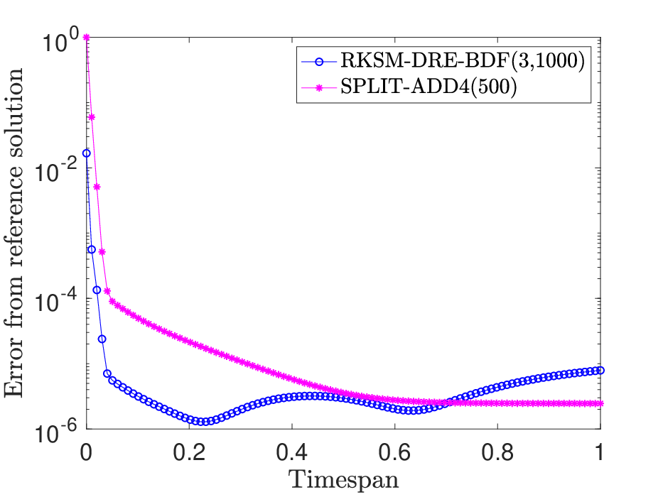
The figures indicate that we compare methods having approximation errors of similar order. The performance results are contained in table 8 for two different discretizations of sym2d and nsym3d.
| # -long | Min/Max | Tot CPU | ||
| Data () | Method | Vecs | rank | time (s) |
| sym2d | rksm-dre | 8 | 3/6 | 0.6 |
| split-add4(500) | 28 | 3/7 | 34.9 | |
| nsym3d | rksm-dre | 10 | 4/7 | 2.2 |
| split-add4(500) | 36 | 3/9 | 37.9 | |
| sym2d | rksm-dre | 6 | 3/4 | 1.2 |
| split-add4(500) | 28 | 3/7 | 330.0 | |
| nsym3d | rksm-dre | 10 | 4/8 | 10.1 |
| split-add4(500) | 36 | 3/9 | 127.8 |
All numbers indicate the competitiveness of rksm-dre in terms of storage and computational time. The memory requirements for split-add4 is measured as the dimension of the solution factor at the final timestep, before column compression. If the solution is required at more time instances, then these memory requirements will increase accordingly.
We also mention that we have experimented with the dynamic splitting methods introduced in [35], however the algorithms proposed by the authors44 4 We thank Chiara Piazzola for providing us with her Matlab implementation of the method. in [35] appeared to be better suited for small to medium size problems.
Discussion on the refinement step. In previous sections, we have stressed that the two approximation stages of the projection method are independent, and we have focused on determining an effective approximation space. Here we linger over the accuracy of the second stage, the refinement step. Exploiting the far smaller problem size of the reduced problem, it is possible to allow for a much more accurate integration phase than what was done during the iteration of the reduction step. This crucial fact is already illustrated in the time break down of tables 4 to 6, where especially for rksm-dre the refinement phase employs a fraction of the overall computational time, while still allowing for a rather accurate final solution.
We next explore in more detail these advantages with rksm-dre on sym2d, where the discretization was further refined to get a coefficient matrix of dimension . The dimensions of the other corresponding matrices remain as presented in table 1. We investigate the time taken by DRE solvers with different accuracies to emphasize the advantages and flexibility of the refinement procedure. table 9 reports the timings for a refinement step performed by three different bdf methods and three splitting methods. The 8th order adaptive splitting method (split-adapt8) also comes from [47] and is performed with a tolerance of , i.e., the same as that of the reduction procedure. We emphasize that in the refinement phase we have utilized some of the most accurate integrators available, and nevertheless the high-dimensional () problem is approximated in less than 200 seconds for all integrators.
| Refinement | # -long | Soln. | Reduction | Refinement | Tot CPU |
|---|---|---|---|---|---|
| Method | Vecs | rank | phase(s) | phase(s) | time(s) |
| bdf(2,100) | 72 | 55 | 37.7 | 1.1 | 38.8 |
| bdf(3,1000) | 72 | 55 | 37.7 | 9.6 | 47.3 |
| bdf(4,10000) | 72 | 55 | 37.7 | 95.5 | 133.2 |
| split-add4(500) | 72 | 55 | 37.7 | 25.9 | 63.6 |
| split-add8(500) | 72 | 55 | 37.7 | 59.6 | 97.3 |
| split-adapt8 | 72 | 55 | 37.7 | 160.7 | 198.4 |
7 Conclusions and open problems
We have devised a rational Krylov subspace based order reduction method for solving the symmetric differential Riccati equation, providing a low-rank approximate solution matrix at selected time steps. A single projection space is generated for all time instances, and the space is expanded until the solution is sufficiently accurate. We stress that our approach is very general, and that it could be applied to subspaces other than Krylov-based ones, as long as the spaces are nested, so that they keep growing as the iterations proceed. This methodology could then be employed for more complex settings, such as parameter dependent problems, where the involved approximation space may require the inclusion of some parameter sampling.
Like in typical model order reduction strategies, in our methodology time stepping is only performed at the reduced level, so that the integration cost is drastically lower than what one would have by applying the time stepping on the original large dimensional problem. We have derived a new stopping criterion that takes into account the different approximation behavior of the algebraic and differential portions of the problem, together with a refinement procedure that is able to improve the final approximate solution by using a high-order integrator. These enhancement strategies have also been applied to the extended Krylov subspace approach. We have analyzed the asymptotic behavior of the reduced order solution, so as to ensure that the generated approximation behaves like the sought after time-dependent solution.
Although our numerical results are promising, there are still several open issues associated with the reduced order solution of the DRE. In particular, while stability and other matrix properties associated with the solutions have been thoroughly studied [10, 19, 37, 16], the analysis of corresponding properties for the approximate solution for is still a largely open problem. In [27] some interesting monotonicity properties have been shown when the polynomial Krylov subspace is used together with particular ODE solvers; a complete analysis for in a more general setting would be desirable.
Acknowledgements
We thank Khalide Jbilou for helpful explanations on [3], and Jens Saak for assistance in using the software M.E.S.S. v.1.0.1 [41]. We are also grateful to Chiara Piazzola for making her code from [35] available and to Tony Stillfjord for pointing us towards his codes from [47]. We thank Maximilian Behr for some helpful criticism on a previous version of this manuscript. The first author acknowledges the insightful comments and kind hospitality of the group of Peter Benner at the Max Planck Institute in Magdeburg (D), during a short visit in February 2019. Furthermore, we thank two anonymous referees for their careful reading and insightful comments.
This research is supported in part by the Alma Idea grant of the Alma Mater Studiorum Università di Bologna, and by INdAM-GNCS under the 2018 Project “Metodi numerici per equazioni lineari, non lineari e matriciali con applicazioni”. The second author is a member of INdAM-GNCS.
Appendix A Krylov subspace properties
In this Appendix we review some properties of extended and rational Krylov subspaces. As in section 2 we denote .
Extended Krylov subspace. The extended Krylov subspace takes the form discussed in section 2. The orthonormal basis spanning the subspace is formed using the extended Arnoldi algorithm [17]. Let
| (22) |
where and is the last columns of . The extended Arnoldi algorithm produces the Arnoldi-type relation
| (23) |
Rational Krylov subspace. The rational Krylov subspace was originally proposed in the eigenvalue context in [39]. Its use in our context is motivated by [45] and later [43], where its effectiveness in the solution of the algebraic Riccati equation is amply discussed.
Assume that is Hurwitz. Given , with , the rational Krylov subspace is given by as defined in section 2. The approximation effectiveness of this subspace depends on the choice of shifts , and this issue has been investigated in the literature; see, e.g., [36], [18]. The adaptive choice of shifts was tailored to the ARE in [32] by the inclusion of information of the term during the shift selection; see also [43] for a more detailed discussion55 5 The Matlab code of the rational Krylov subspace method for ARE is available at http://www.dm.unibo.it/simoncin/software. In our numerical experiments we used this last adaptive strategy, where the approximate solution at timestep is used.
The algorithm presented in [18] forms a complex basis, when the shifts are not all real. In short, when , the original approach would be to use the shift to form the next block and to then let the following shift be given by , where denotes the complex conjugate of . This results in both and being complex. As a consequence, the reduced DRE has complex coefficient matrices, although the final resulting approximations will be real. Standard ODE solvers do not handle complex arithmetic well, hence we implemented an all-real basis using the method introduced in [40], which works as follows. If the shift is complex then the block is also complex, hence we split it into its real and complex parts, that is . The block is then formed by orthogonalizing with respect to all vectors in the already computed basis, after which is formed by orthogonalizing with respect to all previous vectors in in the computed basis, and in . This determines the same space, since spanspan. The resulting real basis of the rational Krylov subspace is given by . We also define the matrices and the matrix
| (24) |
where and holds the last columns of . The matrix contains the orthogonalization coefficients obtained during the rational Arnoldi algorithm.
Let . The rational Krylov basis satisfies the Arnoldi-type relation
| (25) |
where and the matrix is an orthonormal matrix such that
| (26) |
is the decomposition of the matrix on the right (see [18, 31]). The rational Krylov procedure requires as an extra input the (usually real) values , which form a rough approximation of a spectral region used to compute the next shift. The reader is referred to [18, 43] for implementation details. Further, for the computation of the term contained in the residual computation of rksm-dre, we follow an accelerated computation technique presented in [18].
Appendix B Extended Krylov subspace based method
The extended Krylov (eksm-dre) subspace method for solving eq. 1 is presented in algorithm 3.
References
- [1] Oberwolfach model reduction benchmark collection., 2003.
- [2] H. Abou-Kandil, G. Freiling, V. Ionescu, and G. Jank, Matrix Riccati Equations in Control and Systems Theory, Birkhauser, 2003.
- [3] V. Angelova, M. Hached, and K. Jbilou, Approximate solutions to large nonsymmetric differential Riccati problems with applications to transport theory, arXiv preprint arXiv:1801.01291, (2018).
- [4] A. C. Antoulas, Approximation of large-scale dynamical systems, vol. 6, SIAM, 2005.
- [5] M. Behr, P. Benner, and J. Heiland, On an invariance principle for the solution space of the differential Riccati equation, Proc. Appl. Math. Mech., 18 (2018), p. e201800031.
- [6] , Invariant Galerkin ansatz spaces and Davison-Maki methods for the numerical solution of differential Riccati equations, arXiv preprint arXiv:1910.13362, (2019).
- [7] P. Benner, A. Cohen, M. Ohlberger, and K. Willcox, Model reduction and approximation theory and algorithms, SIAM, Philidelphia, 2017.
- [8] P. Benner, V. Mehrmann, and D. Sorensen, Dimension Reduction of Large-Scale Systems, Springer-Verlag, Berlin/Heidelberg, Germany, 2005.
- [9] D. A. Bini, B. Lannazzo, and B. Meini, Numerical solution of algebraic Riccati equations, vol. 9, SIAM, 2012.
- [10] R. Bitmead, M. Gevers, I. Petersen, and J. Kaye, Monotonicity and stabilizability-properties of solutions of the Riccati difference equation: Propositions, lemmas, theorems, fallacious conjectures and counterexamples, Systems & Control Letters, 5 (1985), pp. 309–315.
- [11] S. Blanes, High order structure preserving explicit methods for solving linear-quadratic optimal control problems and differential games, Numerical Algorithms, 69 (2015), pp. 271––290.
- [12] C. Choi and A. Laub, Efficient matrix-valued algorithms for solving stiff Riccati differential equations, IEEE Trans. Automat. Control, 35 (1990), p. 770–776.
- [13] M. J. Corless and A. E. Frazho, Linear systems and control - an operator perspective, Marcel Dekker, New York Basel, 2003.
- [14] E. Davison and M. Maki, The numerical solution of the matrix Riccati differential equation, IEEE Trans Autom Control, (1973), pp. 71–73.
- [15] L. Dieci, Numerical integration of the differential Riccati equation and some related issues, SIAM J. Numer. Anal., 29 (1992), pp. 781–815.
- [16] L. Dieci and T. Eirola, Preserving monotonicity in the numerical solution of Riccati differential equations, Numer Math, 74 (1996), pp. 35–47.
- [17] V. Druskin and L. Knizhnerman, Extended Krylov subspaces: approximation of the matrix square root and related functions, SIAM J Matrix Anal Appl, 19 (1998), pp. 755–771.
- [18] V. Druskin and V. Simoncini, Adaptive rational Krylov subspaces for large-scale dynamical systems, Systems & Control Letters, 60 (2011), pp. 546–560.
- [19] M. Gevers, R. Bitmead, I. Petersen, and J. Kaye, When is the solution of the Riccati equation stabilizing at every instant?, in Frequency Domain and State Space Methods for Linear Systems, North-Holland, 1986, pp. 531–540.
- [20] L. Grasedyck, Existence and computation of low Kronecker-rank approximations for large linear systems of tensor product structure, Computing., 72 (2004), pp. 247–265.
- [21] , Existence of a low rank or -matrix approximant to the solution of a Sylvester equation, Numer. Linear Algebra Appl., 11 (2004), pp. 371–389.
- [22] N. Guglielmi and V. Simoncini, On the existence and approximation of a dissipating feedback, arXiv preprint arXiv:1811.00069, (2019).
- [23] Y. Guldogan, M. Hached, K. Jbilou, and M. Kurulaya, Low rank approximate solutions to large-scale differential matrix Riccati equations, Applicationes Mathematicae, 45 (2018), pp. 233–254.
- [24] M. Heyouni and K. Jbilou, An extended block arnoldi algorithm for large-scale solutions of the continuoustimealgebraic riccati equation, Electron Trans Numer Anal, 33 (2009), pp. 53–62.
- [25] I. M. Jaimoukha and E. M. Kasenally, Krylov subspace methods for solving large Lyapunov equations, SIAM J. Numer. Anal., 31 (1994), pp. 227–251.
- [26] M. Konstantinov and G. Pelova, Sensitivity of the solutions to differential matrix Riccati equations, IEEE Trans. Autom. Control, 36 (1991), pp. 213–215.
- [27] A. Koskela and H. Mena, Analysis of Krylov subspace approximation to large scale differential Riccati equations, arXiv preprint arXiv:1705.07507, (2018).
- [28] V. Kucera, A review of the matrix Riccati equation, Kibernetika, 9 (1973), pp. 42–61.
- [29] H. Kwakernaak and R. Sivan, Linear optimal control systems, vol. 1, Wiley-interscience New York, 1972.
- [30] N. Lang, Numerical methods for large-scale linear time-varying control systems and related differential matrix equations, PhD thesis, Technische Universitaet Chemnitz, 2017.
- [31] Y. Lin and V. Simoncini, Minimal residual methods for large scale Lyapunov equations, Applied Num Math, 72 (2013), pp. 52–71.
- [32] , A new subspace iteration method for the algebraic riccati equation, Numerical Linear Algebra w/Appl., 22 (2015), pp. 26–47.
- [33] The MathWorks, MATLAB 7, r2013b ed., 2013.
- [34] H. Mena, Numerical Solution of Differential Riccati Equations Arising in Optimal Control Problems for Parabolic Partial Differential Equations, PhD thesis, Escuela Politécnica Nacional, 2007.
- [35] H. Mena, A. Ostermann, L.-M. Pfurtscheller, and C. Piazzola, Numerical low-rank approximation of matrix dierential equations, J. Comput. Appl. Math., 340 (2018), pp. 602–614.
- [36] T. Penzl, A cyclic low-rank smith method for large sparse lyapunov equations, SIAM J Sci Comput, 21 (2000), pp. 1401–1418.
- [37] M.-A. Poubelle, R. Bitmead, and M. Gevers, Fake algebraic Riccati techniques and stability, IEEE Trans. Autom. Control, 33 (1988), pp. 379–381.
- [38] W. Reid, Riccati differential equations, Academic Press, New York, 1972.
- [39] A. Ruhe, Rational Krylov sequence methods for eigenvalue computation, Lin. Alg. Appl., 58 (1984), pp. 391–405.
- [40] , The rational Krylov algorithm for nonsymmetric eigenvalue problems. III:Complex shifts for real matrices, BIT, 34 (1994), pp. 165–176.
- [41] J. Saak, M. Köhler, and P. Benner, M-m.e.s.s.-1.0.1 – the matrix equations sparse solvers library. DOI:10.5281/zenodo.50575, Apr. 2016. see also:www.mpi-magdeburg.mpg.de/projects/mess.
- [42] V. Simoncini, A new iterative method for solving large-scale lyapunov matrix equations, SIAM J Sci Comput, 29 (2007), pp. 1268–1288.
- [43] , Analysis of the rational Krylov subspace projection method for large-scale algebraic Riccati equations, SIAM J. Matrix Anal. Appl., 37 (2016), pp. 1655–1674.
- [44] , Computational methods for linear matrix equations, SIAM Rev, 58 (2016), pp. 377–441.
- [45] V. Simoncini, D. B. Szyld, and M. Monsalve, On two numerical methods for the solution of large-scale algebraic Riccati equations, IMA Journal of Numerical Analysis, 34 (2014), pp. 904–920.
- [46] T. Stillfjord, Low-rank second-order splitting of large-scale differential Riccati equations, IEEE Trans Automat Control, 60 (2015), pp. 2791–2796.
- [47] , Adaptive high-order splitting schemes for large-scale differential Riccati equations, Numer Algor, 78 (2018), pp. 1129–1151.
- [48] , Singular value decay of operator-valued differential Lyapunov and Riccati equations, SIAM J. Control Optim., 56 (2018), pp. 3598–3618.