Reconstruction of rational ruled surfaces from their silhouettesThanks: This article was published in Journal of Symbolic Computation, Vol 104, May-June 2021, Authors: Matteo Gallet, Niels Lubbes, Josef Schicho, and Jan Vršek, Title: “Reconstruction of rational ruled surfaces from their silhouettes”, Pages 366–380, DOI:10.1016/j.jsc.2020.08.002, Copyright Elsevier (2020).
© 2020. This manuscript version is made available under the CC-BY-NC-ND 4.0 license http://creativecommons.org/licenses/by-nc-nd/4.0/.Thanks: ∗ Corresponding author.Thanks: ∘ Supported by the Austrian Science Fund (FWF): W1214-N15,
Project DK9.Thanks: ⋄ Supported by the Austrian Science Fund (FWF): P26607 and
P31061.Thanks: ∙ Supported by the Austrian Science Fund (FWF): Erwin
Schödinger Fellowship J4253.Thanks: † Supported by the Austrian Science Fund (FWF): P33003.Thanks: ‡ Supported by project LO1506 of the Czech Ministry of
Education, Youth and Sports.
Abstract.
We provide algorithms to reconstruct rational ruled surfaces in three-dimensional projective space from the “apparent contour” of a single projection to the projective plane. We deal with the case of tangent developables and of general projections to of rational normal scrolls. In the first case, we use the fact that every such surface is the projection of the tangent developable of a rational normal curve, while in the second we start by reconstructing the rational normal scroll. In both instances we then reconstruct the correct projection to of these surfaces by exploiting the information contained in the singularities of the apparent contour.
1. Introduction
Rational ruled surfaces are rational surfaces that contain a straight line through each point. They have been extensively investigated from the point of view of computer algebra, see for example [3], [2], or [17]. When we project to a rational ruled surface , we get a finite cover of branched along a curve, which is the zero set of the discriminant of the equation of along the direction of projection. In this paper, we study the problem of reconstructing the equation of the surface from the discriminant, up to unavoidable projective automorphisms that preserve the discriminant. We have already investigated this question in [8] for a wider class of surfaces, namely the ones admitting at worst ordinary singularities. However, for rational ruled surfaces we are able to create a faster algorithm for reconstruction, based on a completely different technique from the one in [8].
We follow the notation from [8] and we define the contour to be the locus of points on the surface whose tangent space passes though the center of projection. It consists of the singular locus of the surface and of another curve, which we call the proper contour. The projection of the contour is the silhouette of , which splits into the singular image and the proper silhouette. Our goal is then, starting from the knowledge of the singular image and of the proper silhouette, to reconstruct the surface , up to projective automorphisms that preserve the center of projection and the lines through it.
In the remainder of the introduction, we discuss the organization of the paper.
A special subcase of rational ruled surfaces is the one of developables, i.e., surfaces that are either a cone over a plane curve or the union of the tangents of a space curve. In Section 2 we consider the latter case. The main idea is that the projection of the space curve appears as a component with multiplicity three in the discriminant. Our task is to lift this projected curve back to space; we do so by exploiting the information contained in particular singularities of the projection of the nodal curve of the surface. In this subcase, the proper silhouette consists of a union of lines, which are projections of special lines of the surface.
In Section 3 we deal with general projections to of rational normal scrolls. In this case, we first identify the rational normal scroll and construct a projection from it to having the proper silhouette as branching locus. Secondly, we project the rational normal scroll to so that we obtain a double curve as prescribed by the singular image. Notice that the two-dimensional picture of a ruled surface tells more than the picture of an arbitrary surface: the lines of the surface map to tangents to the apparent contour, hence we already get (for free!) projections of all lines of the surface. This is an advantage which we try to keep in our algorithm. The rationality of the given ruled surface implies then that the apparent contour is itself rational. There are well-known algorithms to produce a parametrization, and such a parametrization can also be used to parametrize the set of all tangents, namely its dual curve. The -basis of the parametrization, which was defined and studied in the context of the implicitization problem by [5], gives rise to a rational normal scroll surface, embedded in a projective space of higher dimension. The ruled surface that we wish to compute is then simply a projection of this rational scroll, and the most expensive computations go into figuring out this final projection.
We conclude the paper by recalling in Section 4, for the benefit of the reader, a known algorithm for the parametrization of curves which we implement ad hoc in our algorithm, since currently available general-purpose algorithms for parametrizations of plane curves do not exploit the special structure of the curves we deal with. This determines a relevant speed-up of our algorithm, since the parametrization of a particular planar curve constitutes its computational bottleneck.
An implementation in Maple of the algorithms developed in this paper is available at
https://www.risc.jku.at/people/jschicho/pub/ChisiniRuled.mpl.
2. Tangent developable surfaces
Among ruled surfaces, developable surfaces can be characterized as follows. A line of a ruled surface is called torsal if all tangent planes at all smooth points of the line are equal; a developable surface is then a ruled surface such that all lines of the surface are torsal.
A developable surface is either a tangent developable, i.e., the union of all tangents of a space curve (Figure 1), or a cone over a planar curve — see [11, Chapter IV, Section 30] and [19, Theorem 0], or [1, Proposition 2.12] for a proof in terms of algebraic geometry. In this section, we recognize general rational tangent developables from their silhouettes with respect to general projections. The case of cones is equivalent to the recognition of a planar algebraic curve from its branching points with respect to a projection to the projective line.
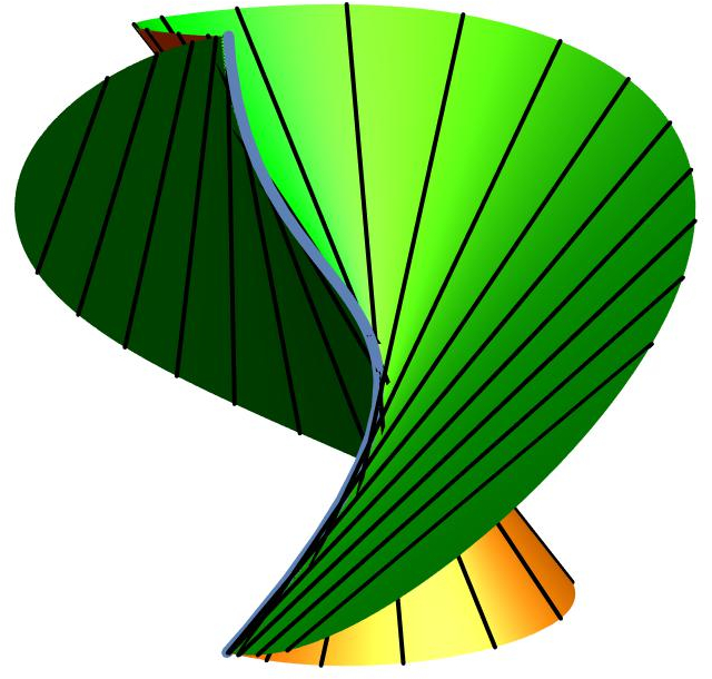
Let . Every tangent developable of a rational curve of degree is a projection of the tangent developable of the rational normal curve of degree in . The surface has degree and admits a parametrization of the form
The surface contains the rational normal curve as a cuspidal singularity, namely locally analytically the surface around such a curve looks like a cylinder over a plane cusp. Hence tangent developables have a whole curve composed of cuspidal singularities, which is the projection of the rational normal curve in . We call this curve the cuspidal curve, and we notice that it is a rational curve. Tangent developables may have other singularities, coming from the fact that they are projections of , such as self-intersecting curves. Locally analytically around a point of a self-intersection curve, the tangent developable has two branches that intersect transversally. This is why we call these curves of singularities nodal curves.
Here we describe the tangent developables in we intend to recognize: we prescribe their singularities having in mind the situation of a general projection of to . We call a tangent developable in good if it satisfies the following conditions:
-
the only singularities of the tangent developable are contained in the cuspidal curve, and in the nodal curve;
-
the cuspidal curve is smooth and irreducible;
-
the nodal curve is irreducible and has only ordinary triple points, or singular points as described in the next item;
-
the points of intersection of the nodal curve and the cuspidal curve belong to one of the following two types:
- –
points for which the local analytic equation of the surface at the point is equivalent to ; in this local equation, the point is the origin, the cuspidal curve is and the nodal curve is ; as the local equation shows, the nodal curve has a cusp at the intersection point (see Figure 2(a));
- –
points that are a transversal intersection of the nodal and the cuspidal curves at a “cuspidal pinch point”; the local analytic equation at such a point is equivalent to (see Figure 2(b));
- –
-
there are exactly cuspidal pinch points.
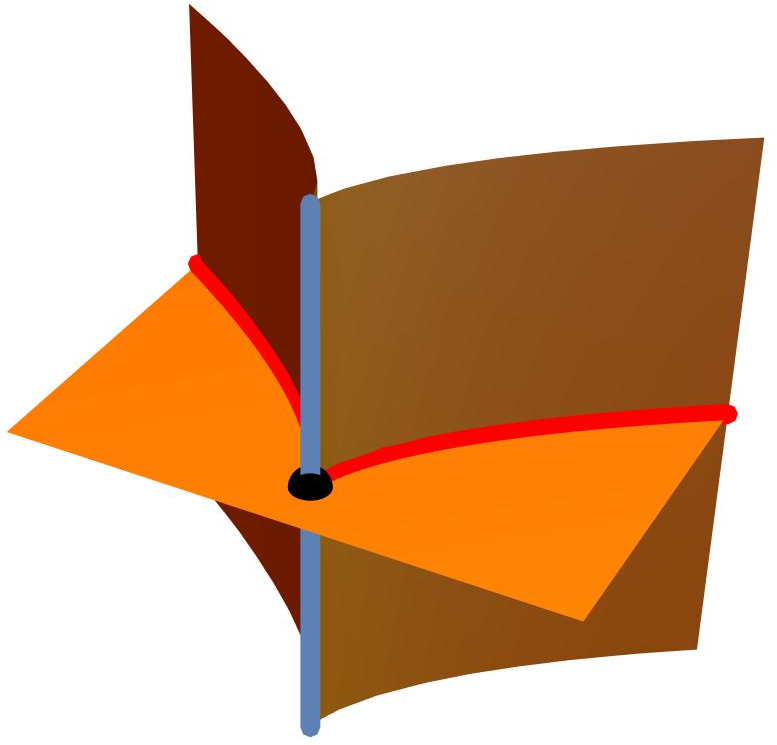

Now we examine the silhouette with respect to a general projection to of a good tangent developable surface. In the algorithm we are going to develop (Algorithm ReconstructTangentDevelopable), we use the knowledge of the two components of the silhouette to reconstruct the tangent developable.
Definition 2.1.
Let be a good tangent developable surface. The image of the cuspidal curve of under a projection to is called the cuspidal image; the image of the nodal curve of is called the nodal image.
Proposition 2.2.
If is a good tangent developable surface, then the discriminant of a general projection11 1 The discriminant of a projection is the polynomial defining the locus of points such that the preimage of under is tangent to . If, in coordinates, the projection is given by the map and is the equation of , then the discriminant of is the discriminant of with respect to . of to has the following factors:
-
a factor of multiplicity three, whose zero set is the cuspidal image;
-
a factor of multiplicity two, whose zero set is the nodal image;
-
several linear factors of multiplicity one, which are images of tangent planes passing through the center of projection; their zero set is the proper silhouette of the projection.
Proof.
A general projection of a cusp is a triple zero of the discriminant, hence the cuspidal image is a triple component. Similarly, a general projection of a node is a double zero of the discriminant, hence the nodal image is a double component. Both these two results follow from a local analysis of the situation. In fact, locally around a general point of the cuspidal curve, we can take coordinates so that the equation of the surface is and the projection is along , so the discriminant is ; similarly, locally around a general point of the nodal curve, we can take the equation of the surface to be , and the projection along , so that the discriminant is . Since all lines are torsal, namely all the tangent planes at points of one of these lines coincide, the proper contour is composed of lines, and their images determine the linear factors of the discriminant. ∎
The lines in the proper silhouette are inflection tangent lines of the cuspidal image. The intersections of the cuspidal image and the nodal image are either cusps of the nodal image or transverse intersections coming from transverse intersections of nodal and cuspidal curve, or from pairs of distinct point, each on one of the two curves, collapsed by the projection. Apart from these intersections, and from triple points on the nodal image, we allow the cuspidal image and the nodal image to have only ordinary double points.
The recognition problem of a tangent developable reduces to the construction of the cuspidal curve from the factors of the discriminant. The cuspidal curve is the projection of a rational normal curve of the same degree . This projection is given by four polynomials of degree of which we already know three, namely those that define the projection to the cuspidal image in . In order to find the fourth polynomial, we have to use the nodal image. Notice, in fact, that the inflection lines do not add any information: any choice of a fourth polynomial would lead to the same linear factors of the discriminant.
The basic idea of Algorithm ReconstructTangentDevelopable is to collect linear conditions for the fourth polynomial derived from cuspidal pinch points. Their projections to are transversal intersections of the nodal image with the cuspidal image. Hence, we try every possible subset of cardinality of the set of all transversal intersections. Notice that if the cuspidal curve is defined over , then the images of the cuspidal pinch points are all conjugated over , so it is easy to extract them from the set of all intersections. Suppose that the three polynomials giving the parametrization of the cuspidal image are , and . Then the fourth polynomial can be found as follows: we make a symbolic ansatz for its coefficients and compute the determinant of the matrix
| (1) |
This determinant vanishes at the parameters corresponding to images of the cuspidal pinch points (see Remark 2.3). Imposing this vanishing for all points of a subset of cardinality of transversal intersections of the nodal image with the cuspidal image provides linear conditions for the coefficients of . We show in Lemma 2.4 that the space of solutions of these linear equations is -dimensional. This means that the choice of is unique up to linear combinations of , , and . In turn, this clarifies that the reconstruction of the cuspidal curve (and hence of the tangent developable) performed by Algorithm ReconstructTangentDevelopable is unique up to projective transformations of that preserve the silhouette.
We would like to point out that Algorithm ReconstructTangentDevelopable relies on nontrivial “basic” operations in computational algebraic geometry, as computing a parametrization of a rational curve, or computing and manipulating the intersection of two plane curves. These are, in general, difficult independent problems for which there is a vast literature, and that are objects of active research; we consider them as “building blocks” of our algorithm.
Notice that, in order to perform Step , one may plug the parametrization of into the equation of , hence obtaining an equation in a single variable. Then this equation may be solved (symbolically, which may need the introduction of algebraic numbers, or numerically), and the solutions provide the points of intersection of and .
Remark 2.3.
Consider a nondegenerate rational curve of degree in , and a point , which we can suppose to be . A local parametrization of around is of the form with . We may assume that up to linear changes of coordinates. We say that is special if . The multiplicity of a special point is defined as , and one has that the sum of multiplicities of special points of equals (see [9, Definition 3.4 and Lemma 3.6]). A general rational curve of degree in has exactly special points of multiplicity (see [9, Lemma 3.5]), and a local parametrization of at these points is of the form . These points determine the cuspidal pinch points of tangent developable of .
Lemma 2.4.
The dimension of the solution space to the linear system in Algorithm ReconstructTangentDevelopable is .
Proof.
The dimension is at least since we suppose that we start from a projection of a tangent developable. In particular, there exists a rational curve of degree in parametrized by where the are linearly independent elements in the solution space. By assumption, the curve admits exactly special points of multiplicity : in fact, if has a special point of multiplicity , we see from its local parametrization that the tangent developable of has a cuspidal pinch point at . Suppose, by contradiction, that the dimension of the solution space is at least . This implies that there exists a rational curve of degree in projecting to . The curve has at least special points that remain special after projection to . Therefore, these points must be of multiplicity at least . This follows from the fact that special points of multiplicity project to non-special points, since any multiplicity point on the curve has local parametrization of type ; these points project to points in around which the parametrization is , and so they are non-special. The sum of multiplicities of special points in must give , but this is a contradiction, since for . ∎
Remark 2.5.
Notice that there is no nodal curve in the tangent developable of a twisted cubic, and thus no special points in its cuspidal curve. However, Lemma 2.4 is trivially true for since the space of univariate polynomials of degree at most is -dimensional.
3. General projections of rational normal scrolls
In this section, we provide a reconstruction algorithm for rational ruled surfaces that admit particularly simple singularities. Recall from the introduction that, given a projection , we call contour the locus of points on whose tangent plane passes though the center of projection. The contour is the union of singular locus of the surface and of the proper contour. The image of the contour under the projection is the silhouette; it is constituted of the singular image (the image of the singular locus) and the proper silhouette (the image of the proper contour). In this section, we consider good rational ruled surfaces and good projections , namely we ask that:
-
has at most ordinary singularities: an irreducible self-intersection curve, self-intersection triple points, and pinch points;
-
the proper silhouette has only nodes and cusps;
-
the singular image has only nodes and ordinary triple points;
-
the proper contour is irreducible and projects birationally to the proper silhouette;
-
the singular curve projects birationally to the singular image.
Recall that every rational ruled surface is a projection of a rational normal scroll. Our assumptions imply that the restriction of this projection to its ramification locus is generically injective. Notice that all our assumptions are fulfilled when we consider projections from general centers (both when we project from the rational normal scroll to , and when we project from the surface to ). In particular, irreducibility of the singular curve is Franchetta’s Theorem (see [14, Theorem 6]). The fact that good rational ruled surfaces have ordinary singularities implies that they have finitely many torsal lines, each passing through exactly one pinch point.
We divide the reconstruction process in two steps: first, we determine the rational normal scroll of which the surface is a projection, together with the projection from this rational normal scroll to , by computing a parametrization of the dual of the proper silhouette, which is a rational curve; second, we construct the projection map from the rational normal scroll to the surface in .
 |
To explain how the first part of the reconstruction works, we recall some facts about rational normal scrolls.
For our purposes, we use the description of rational normal scrolls provided by [4, Example 2.3.16]: given two natural numbers , the rational scroll is the Zariski closure of the image of the map
In this way, a linear projection can be identified with two vectors of polynomials of degrees and so that the map
| (2) |
fits into the commutative diagram
Since the projection is a map between smooth varieties, the notions analogous to the ones of contour and silhouette for projections are usually called, in this case, the ramification locus and the branching locus, respectively. Hereafter, we collect some pieces of information about the branching locus of such a projection. The following result is well-known, but we report the proof, since we could not find a reference asserting exactly the fact we need.
Lemma 3.1.
Let be a projection from a rational normal scroll whose restriction to the ramification locus is generically injective. Then every line in is projected by to a tangent line of the branching locus.
Proof.
Let be a line. By hypothesis, we know that and are both generically injective because any projection whose center is not in is generically injective on the lines of the surface. Let be a smooth point of , then is tangent to at . In fact, by definition, the tangent plane of at intersects the center of projection. The tangent line of at and are both contained in this tangent plane. The projection either collapses the tangent line of . In the first case, since is generically injective, and there are no birational maps between smooth curves collapsing tangent vectors, it follows that is singular in . Therefore the statement is trivially true. In the second case, both and the tangent line of are projected to a single line in , which equals . Hence is tangent to at . ∎
The next proposition provides the first part of the reconstruction algorithm. We are going to use the concept of -bases, introduced by Cox, Sederberg and Chen in [5]: these are particular sets of generators of the module of syzygies of a parametrization of a curve or of a surface; we refer to the original paper for a more precise definition and for their properties.
Proposition 3.2.
Let be the branching locus of a projection whose restriction to the ramification locus is generically injective. Let be a -basis of a parametrization of , the dual curve of . Then the projection induced by has as branching locus. Moreover, every general projection having as branching locus is projectively equivalent to over , namely there exists a projective automorphism such that fixes all linear spaces of dimension through the center of projection, which has dimension .
Proof.
We first show that is the branching locus of the map obtained from . By the properties of -bases (see [18, Theorem 2]), the vector gives a parametrization of . This implies that the projection sends the lines of to the family of tangent lines of . In fact, the Plücker coordinates of the line between and are given by . By Lemma 3.1, the curve is the branching locus of . Suppose that is another general projection having as branching locus. Let be the two vectors of polynomials defining as explained in Equation (2). By Lemma 3.1, the images of the lines of are lines tangent to . Hence, by the same argument as before, is a parametrization of . Thus is a -basis of this parametrization. By the uniqueness of -bases, it follows that and , and that and differ by an automorphism over . ∎
Proposition 3.2 tells us that, in order to reconstruct the rational normal scroll of which the desired surface in is a projection it is enough to compute a -basis of a parametrization of the dual of the proper silhouette.
This concludes the first part of the reconstruction process, and proves the correctness of Algorithm ReconstructRationalScroll: there, instead of computing the map , we compute the map as in Equation (2), which provides the same information. In fact, the proper silhouette of a projection is the branching locus of the corresponding projection .
As a consequence of Algorithm ReconstructRationalScroll, we obtain a characterization of proper silhouettes of good projections , where is a good rational ruled surface.
Proposition 3.3.
Proper silhouettes of good projections of good rational ruled surfaces are rational plane curves with maximal number of cusps for a given degree and only ordinary nodes as the other singularities.
Proof.
Let be a proper silhouette of a good projection , where is a good rational ruled surface. We know that the degree of the proper silhouette is , where . We can obtain this number by considering the degree of the silhouette, which is , and subtracting from it twice the degree of the singular image, which is (see [15, Section 6]). If we denote by the number of nodes of and by the number of cusps of , then from the rationality of and the Plücker formulas we get
where is the degree of the dual of . Since the dual of is in fact a plane section of the dual of , and the dual of a ruled surface is a ruled surface of the same degree, we conclude that . These two equations imply that . On the other hand, we know that for a rational curve of degree the number of cusps must be less than or equal to (see [13, Section 5] and [12, Section 4]). Hence proper silhouettes of rational ruled surfaces are rational curves with maximal number of cusps for a given degree.
Conversely, if we are given a rational curve of degree , where is of the form for some , having ordinary cusps and only ordinary nodes as the other singularities, then we can apply Algorithm ReconstructRationalScroll to it, thus showing that such a curve is the silhouette of the projection of a rational ruled surface whose restriction to the ramification locus is generically injective. ∎
Now that, recalling Equation (2), we reconstructed the map via Algorithm ReconstructRationalScroll, we proceed by recovering the projection . To do so, we need to use the information provided by the singular image, namely the projection on of the singular locus of . We formulate two different algorithms to construct this projection: one (Algorithm CollapseMates) imposes the projection to collapse pairs of points in in order to create a prescribed double curve; the other (Algorithm UsePinchPoints), instead, forces the differential of the projection to be rank-deficient at the preimages of pinch points.
Recall that the double curve of is irreducible by assumption. This implies that, in presence of pinch points, the curve in that is mapped to the singular curve of is also irreducible, because the two sheets of the double cover meet precisely at the preimages of the pinch points. Let be the singular image of a good projection , where is a good rational ruled surface. Let be the curve that is mapped to the singular curve of . The curve has bidegree
In fact, by the so-called double point formula (see [7, Section 9.3] for the general formula, and [6, Chapter 10, Equation 10.52] for a specialization of the formula in our case) its divisor class is given by , where is the class of a hyperplane section of and is the class of a line; the bidegree of then follows from the fact that has bidegree and has bidegree .
For any general point there is a unique such that is a fiber of the double cover of . Note that the restriction of to is also a map whose fibers are equal to the fibers of . This allows us to compute in terms of using . We say that is the mate of .
In order to express the conditions imposed by our algorithm more explicitly, we can assume without loss of generality that the projection is the map forgetting the last coordinate. Notice that the map is defined by four linear forms, three of which we already know from the map obtained via Algorithm ReconstructRationalScroll. Let , , and be the known forms, and let be the form to be determined. For every general point and its mate , we get a linear condition in the coefficients of by requiring that the map collapses and , namely by asking that
The forms , , and also satisfy this linear condition, so we look for a solution of the linear system that is linearly independent from , , and .
We claim that the dimension of the solution space for the linear system above is not bigger than . Assume, indirectly, that there is a fifth linearly independent form satisfying the linear equations defined above. Then, the image of the map defined by , , , , and is a nondegenerate rational ruled surface with a double curve of the same degree as the double curve of , namely . Moreover, the projection from to is birational once restricted to the two surfaces. This contradicts the following lemma.
Lemma 3.4.
Let be a projection of a rational normal scroll satisfying our assumptions, namely is a good rational ruled surface. Suppose that factors through a projection to , namely that where and . Then has at most isolated singularities.
Proof.
Assume by contradiction that has a singular curve. Consider a general plane section of and its preimage . Both and have the same geometric genus because they are birational. By Bertini’s theorem, since is the projection of a smooth projective variety, the singularities of are exactly at the intersection with the singular locus of , and their number is . Since (see [15, Section 6]), and we know that is rational, it follows from the geometric genus formula (see [10, Chapter IV, Exercise 1.8(a)]) that the delta invariant of each of the singularities of is . The sum of delta invariants of singularities of the space curve must be strictly smaller than the sum of the delta invariants of the singularities of . This follows from the geometric genus formula, since the arithmetic genus of is bigger than the arithmetic genus of , which cannot be greater than (see [10, Chapter IV, Theorem 6.4 and Figure 18]). It follows that the singular locus must have strictly lower degree than , because every intersection of and determines a singularity of . This implies the image of under the projection to is a component of , but by assumption is irreducible. This contradiction concludes the proof. ∎
From an algorithmic point of view, to obtain the desired projection , we need to find a solution of the infinitely many linear equations above (one for each pair of mates) that is linearly independent from , , and . We could just collect sufficiently many points on and solve the linear equations arising from them and their mates. However, finding points on is not trivial. What we do instead is to compute the mate of a point with coordinates in a transcendental field extension of the base field that is isomorphic to the function field of . More concretely, the equations
allow one to write the coordinates of the mate of a point as rational functions of and . This is a consequence of the fact that whenever we have a map between two curves, then there exists a birational automorphism of swapping the two points in any fiber. This leads to a single linear equation for with coefficients in this function field. Using Gröbner bases, we can eliminate from this single equation the generators of the function field and obtain an equivalent system of linear equations with scalar coefficients.
The discussion so far proves the correctness of Algorithm CollapseMates.
The second algorithm we propose is based on the observation that the fourth unknown polynomial satisfies particularly simple equations coming from pinch points: the Jacobian of the projection is rank-deficient at the preimages of pinch points, more precisely the tangent line of at those points is collapsed to a point by the map defined by .
For this algorithm to work, we need to suppose that the images of pinch points under the projection are transversal intersections of the proper silhouette and the singular image. This is true for projections from general centers (see [8, Proposition 2.1] and the discussion before for a more thorough analysis).
The algorithm works as follows: for each intersection of the proper silhouette and the singular image coming from a pinch point, one considers the corresponding point that is sent to by . Notice that is unique by assumption, since comes from a pinch point. The point lies on the curve which is mapped to the singular image by . We compute the tangent line of at , and we impose that the differential of the map sends it to zero. In this way, we obtain linear conditions for the coefficients of . Solving these linear system provides the desired parametrization of . Notice that we do not know a priori which transversal intersections of the proper silhouette and the singular image come from pinch points, therefore in principle one may have have to repeat the previous procedure for all possible subsets of transversal intersections of proper silhouette and singular image (recall that we suppose from the beginning that the number of pinch points is ). We hence get the following algorithm.
We show that the solution space for the linear equations in Step is exactly four-dimensional, thus proving the correctness of the algorithm. The dimension of this solution space is at least because we know by hypothesis that there is a good projection whose components satisfy the linear conditions. Proposition 3.2 implies that the dimension cannot be bigger than .
We propose an alternative proof of this fact, based on the torsal lines on the ruled surface, which reveals some of the underlying geometry of these surfaces. The proof that the dimension cannot be bigger goes in two steps: first, we show that lines in passing through critical values22 2 Recall that the critical values of a differentiable map are the images of the points at which the differential of the map does not have maximal rank. of the projection are torsal, and secondly we prove that a surface in with too many torsal lines must be degenerate.
Recall from Equation (2) that a projection can be encoded in two vectors of polynomials via the map
in such a way that and are linearly independent for every . The map is singular at the point if and only if the matrix
has rank at most .
Lemma 3.5.
Let and let be a projection entering in a commutative diagram of projections
where the image of is a good rational ruled surface. Suppose that is singular at . Then lies on a torsal line of .
Proof.
Recalling notation introduced above and the fact that a line is torsal when the tangent planes of the ruled surface at each of its points coincide, we have to prove that the matrix
has rank , where are the coordinates of . Since is singular at , this matrix cannot have rank . On the other hand, if this matrix had rank , then the line in passing through would be singular. However, there are no singular lines in , since otherwise also the image of would have singular lines, and this is not allowed by our general assumption. ∎
Lemma 3.6.
Let be a rational ruled surface in with at least torsal lines. Suppose that there exists a projection where is a rational ruled surface with at most ordinary singularities. Then is degenerate, namely it is contained in a hyperplane.
Proof.
The surface is the image of a projection from a rational normal scroll. Let , as above, be the two vectors of polynomials of degree and , respectively, encoding the projection . Torsal lines in correspond to values such that the matrix
has rank at . These values are precisely the common zeros of the determinants of the submatrices obtained by removing a row from the previous matrix. The degree of these determinants (as polynomials in ) is at most . In fact, elementary column operations transform the previous matrix into
and . Hence all the five determinants are of the form for and . The kernel of contains the element
thus and similarly for . Hence all the points of the form are contained in a hyperplane, namely is degenerate. ∎
We can now prove that the solution space for the polynomial defining the map is exactly four-dimensional. In fact, if it were bigger, we would get a projection which is singular at all points that are preimages of the transversal intersections of the proper silhouette and the singular image coming from pinch points of . By [15, Section ], the surface has pinch points. By Lemma 3.5, they determine torsal lines in . Lemma 3.6 shows the contradiction.
The discussion so far proves the correctness of Algorithm UsePinchPoints.
We can sum up the findings of this section in the following algorithm, which reconstructs, up to projective automorphisms preserving the silhouette, a good rational ruled surface starting from the singular image and the proper silhouette of a good projection :
4. A faster parametrization for the silhouette
The bottleneck of Algorithm ReconstructRationalScroll is the computation of the parametrization of the dual of the silhouette. Our situation is quite special: by assumption the silhouette admits only nodes and cusps. General-purpose algorithms for parametrizing curves (as, for example, the one implemented in Maple), do not have the possibility to take into account this special structure of the curve. This is why we implement an ad hoc procedure for the parametrization of the silhouette that uses the fact that we only have nodes and cusps. Although the methods used are all known, we believe it could be beneficial for the reader to have an overview of this algorithm.
We use the well-known technique of adjoints to compute the parametrization, see [16, Section 4.7]. Given a planar curve of degree with only nodes and cusps, the linear system of adjoints is given by those homogeneous forms of degree that pass through the singularities of . In order to get the adjoint forms, we have to take the homogeneous component of degree of the radical of the Jacobian ideal of . One way to obtain this radical ideal is the following: consider the discriminant of the curve along a random projection; this is a bivariate homogeneous polynomial whose factors of order correspond to nodes of and whose factors of order correspond to cusps of . If we add the form to the Jacobian ideal of , then we get its radical. The image of under the rational map induced by the linear system of adjoints is a rational normal curve in of degree . Suppose now that a smooth point is known. Then we get a point in , and the projection from maps to a rational normal curve in of degree . Since the projection is a map between smooth curves, it can be extended also to , which gets mapped to the image of the tangent line under the projection. In this way we obtain a point , so we can repeat the procedure until we land on :
In this way, we get a map , whose inverse is the desired parametrization. Notice that the map can be computed by selecting those adjoint forms that vanish with multiplicity at .
This discussion leads to the following algorithm:
We implemented the algorithms in Maple and tested it on a computer with an Intel I7-5600 processor (1400 MHz). We report the timings in Table 1.
| time | type | ||||||||
| - | - | - | s | developable | |||||
| - | - | - | s | developable | |||||
| - | - | - | s | developable | |||||
| - | - | - | s | ruled | |||||
| - | - | - | s | ruled |
References
- [1] E. Arrondo. Subvarieties of Grassmannians. 1996. URL: http://www.mat.ucm.es/˜arrondo/trento.pdf.
- [2] L. Busé, M. Elkadi, and A. Galligo. A computational study of ruled surfaces. J. Symbolic Comput., 44(3):232–241, 2009. doi:10.1016/j.jsc.2007.04.005.
- [3] F. Chen, J. Zheng, and T. W. Sederberg. The mu-basis of a rational ruled surface. Comput. Aided Geom. Design, 18(1):61–72, 2001. doi:10.1016/S0167-8396(01)00012-7.
- [4] D. A. Cox, J. B. Little, and H. K. Schenck. Toric varieties, volume 124 of Graduate Studies in Mathematics. American Mathematical Society, Providence, RI, 2011. doi:10.1090/gsm/124.
- [5] D. A. Cox, T. W. Sederberg, and F. Chen. The moving line ideal basis of planar rational curves. Comput. Aided Geom. Design, 15(8):803–827, 1998.
- [6] I. V. Dolgachev. Classical algebraic geometry. A modern view. Cambridge University Press, Cambridge, 2012. doi:10.1017/CBO9781139084437.
- [7] W. Fulton. Intersection theory, volume 2 of Ergebnisse der Mathematik und ihrer Grenzgebiete. 3. Folge. A Series of Modern Surveys in Mathematics. Springer-Verlag, Berlin, second edition, 1998. doi:10.1007/978-1-4612-1700-8.
- [8] M. Gallet, N. Lubbes, J. Schicho, and J. Vršek. Reconstruction of surfaces with ordinary singularities from their silhouettes. SIAM J. Appl. Algebra Geom., 3(3):472–506, 2019. doi:10.1137/18M1220911.
- [9] M. Gallet and J. Schicho. Counting projections of rational curves. 2017. URL: https://arxiv.org/abs/1707.05264.
- [10] R. Hartshorne. Algebraic geometry, volume 52 of Graduate Texts in Mathematics. Springer-Verlag, New York-Heidelberg, 1977.
- [11] D. Hilbert and S. Cohn-Vossen. Geometry and the imagination. Chelsea Publishing Company, New York, 1952. Translated by P. Neményi.
- [12] T. R. Hollcroft. The existence of algebraic plane curves. Bull. Amer. Math. Soc., (8):503–521, 1937. doi:10.1090/S0002-9904-1937-06584-0.
- [13] S. Lefschetz. On the existence of loci with given singularities. Trans. Amer. Math. Soc., 14(1):23–41, 1913. doi:10.2307/1988767.
- [14] E. Mezzetti and D. Portelli. A tour through some classical theorems on algebraic surfaces. An. Ştiinţ. Univ. Ovidius Constanţa Ser. Mat., 5(2):51–78, 1997.
- [15] R. Piene. Singularities of some projective rational surfaces. In Computational methods for algebraic spline surfaces, pages 171–182. Springer, Berlin, 2005. doi:10.1007/3-540-27157-0_12.
- [16] J. R. Sendra, F. Winkler, and S. Pérez-Díaz. Rational algebraic curves. A computer algebra approach, volume 22 of Algorithms and Computation in Mathematics. Springer, Berlin, 2008. doi:10.1007/978-3-540-73725-4.
- [17] L.-Y. Shen and S. Pérez-Díaz. Characterization of rational ruled surfaces. J. Symbolic Comput., 63:21–45, 2014. doi:10.1016/j.jsc.2013.11.003.
- [18] N. Song and R. Goldman. -bases for polynomial systems in one variable. Comput. Aided Geom. Design, 26(2):217–230, 2009. doi:10.1016/j.cagd.2008.04.001.
- [19] V. Ushakov. Developable surfaces in Euclidean space. J. Austral. Math. Soc. Ser. A, 66(3):388–402, 1999.