A Graph Theoretic Additive Approximation of Optimal Transport

Transportation cost has been successfully used as a measure of similarity between data sets such as point clouds, probability distributions, and images. Originally studied in operations research, the transportation problem is a fundamental problem where we are given a set $A$ of ‘demand’ nodes and a set $B$ of ‘supply’ nodes with a non-negative demand of $d_{a}$ at node $a\in A$ and a non-negative supply $s_{b}$ at node $b\in B$. Let $G(A,B)$ be a complete bipartite graph on $A,B$ with $n=|A|+|B|$ where $c(a,b)\geq 0$ denotes the cost of transporting one unit of supply from $b$ to $a$; we assume that $C$ is the largest cost of any edge in the graph. We assume that the cost function is symmetric, i.e., $c(a,b)=c(b,a)$. Due to symmetry in costs, without loss of generality, we will assume throughout that the total supply is at most the total demand. Let $U=\sum_{b\in B}s_{b}$. A transport plan is a function $\sigma:A\times B\rightarrow\mathbb{R}_{\geq 0}$ that assigns a non-negative value $\sigma(a,b)$ to every edge $(a,b)$ with the constraints that the total supply coming into any node $a\in A$ is at most $d_{a}$, i.e., $\sum_{b\in B}\sigma(a,b)\leq d_{a}$ and the total supply leaving a node $b\in B$ is at most $s_{b}$, i.e., $\sum_{a\in A}\sigma(a,b)\leq s_{b}$. A maximum transport plan is one where, for every $b\in B$, $\sum_{a\in A}\sigma(a,b)=s_{b}$, i.e., every available supply is transported. The cost incurred by any transport plan $\sigma$, denoted by $w(\sigma)$ is $\sum_{(a,b)\in A\times B}\sigma(a,b)c(a,b)$. In the transportation problem, we wish to compute the minimum-cost maximum transport plan.

There are many well-known special versions of the transportation problem. For instance, when all the demands and supplies are positive integers, the problem is the Hitchcock-Koopmans transportation problem. When the demandname.texual to $1$, i.e., $U=1$. This is the problem of computing optimal transport distance between two distributions. When the cost of transporting between nodes is a metric, the optimal transport cost is also the Earth Mover’s distance (EMD). If instead, the costs between two nodes is the $p$-th power of some metric cost with $p>1$, the optimal transport cost is also known as the $p$-Wasserstein’s distance. These special instances are of significant theoretical interest  [1, 17, 20, 24, 28, 29] and also have numerous applications in operations research, machine learning, statistics, and computer vision [5, 6, 7, 10, 13, 27].

Related work: There are several combinatorial algorithms for the transportation problem. The classical Hungarian method computes an optimal solution for the assignment problem by using linear programming duality in $\mathcal{O}(n^{3})$ time [18]. In a seminal paper, Gabow and Tarjan applied the cost scaling paradigm and obtained an $\mathcal{O}(n^{2.5}\log(nC))$ time algorithm for the assignment problem [14]. They extended their algorithm to the transportation problem with an execution time of $\mathcal{O}((n^{2}\sqrt{U}+U\log U)\log(nC))$; their algorithm requires the demands, supplies and edge costs to be integers. For the optimal transport problem, scaling the demands and supplies to integers will cause $U$ to be $\Omega(n)$. Therefore, the execution time of the GT-Algorithm will be $\Omega(n^{2.5})$. Alternatively, one could use the demand scaling paradigm to obtain an execution time of $\mathcal{O}(n^{3}\log U)$ [12]. For integer supplies and demands, the problem of computing a minimum-cost maximum transport plan can be reduced to the problem of computing a minimum-cost maximum flow, and applying the result of [21] gives a $\tilde{\mathcal{O}}(n^{2.5}\mathrm{poly}\log(U))$¹¹ 1 We use the notation $\tilde{\mathcal{O}}$ to suppress additional logarithmic terms in $n$. time algorithm.

We would also like to note that there is an $\mathcal{O}(n^{\omega}C)$ time algorithm to compute an optimal solution for the assignment problem [23]; here, $\omega$ is the exponent of matrix multiplication time complexity. With the exception of this algorithm, much of the existing work for exact solutions have focused on design of algorithms that have an execution time polynomial in $n,\log U$, and $\log C$. All existing exact solutions, however, are quite slow in practice. This has shifted focus towards the design of approximation algorithms.

Fundamentally, there are two types of approximate transport plans that have been considered. We refer to them as $\delta$-approximate and $\delta$-close transport plans and describe them next. Suppose $\sigma^{*}$ is a maximum transport plan with the smallest cost. A $\delta$-approximate transport plan is one whose cost is within $(1+\delta)w(\sigma^{*})$, whereas a transport plan $\sigma$ is $\delta$-close if its cost is at most an additive value $U\delta$ larger than the optimal, i.e., $w(\sigma)\leq w(\sigma^{*})+U\delta$. Note that, for discrete probability distributions $U=1$, and, therefore, a $\delta$-close solution is within an additive error of $\delta$ from the optimal.

For metric and geometric costs, there are several algorithms to compute $\delta$-approximate transport plans that execute in time near-linear in the input size and polynomial in $(\log n,\log U,\log C)$. For instance, $\delta$-approximate transport plans for the $d$-dimensional Euclidean assignment problem and the Euclidean transportation problem can be computed in $n(\log n/\delta)^{\mathcal{O}(d)}\log U$ time [17, 28]. For metric costs, one can compute a $\delta$-approximate transport plan in $\tilde{\mathcal{O}}(n^{2})$ time [1, 30]. There are no known $\delta$-approximation algorithms that execute in near-linear time when the costs are arbitrary.

There are several algorithms that return $\delta$-close transport plan for any arbitrary cost function. Among these, the best algorithms take $\tilde{\mathcal{O}}(n^{2}(C/\delta))$ time. In fact, Blanchet et al. [8] showed that any algorithm with a better dependence on $C/\delta$ can be used to compute a maximum cardinality matching in any arbitrary bipartite graph in $o(n^{5/2})$ time. Therefore, design of improved algorithms with sub-linear dependence on $(C/\delta)$ seems extremely challenging. See Table 1 for a summary of various results for computing a $\delta$-close transport plan. Note that all previous results have one or more factors of $\log n$ in their execution time. While some of these poly-logarithmic factors are artifacts of worst-case analyses of the algorithms, one cannot avoid them all-together in any practical implementation.

Due to this, only a small fraction of these results have reasonable implementation that also perform well in practical settings. We would like to highlight the results of Cuturi [9], Altschuler et al. [3], and, Dvurechensky et al. [11], all of which are based on the Sinkhorn projection technique. All these implementations, however, suffer from a significant increase in running time and numerical instability for smaller values of $\delta$. These algorithms are practical only when $\delta$ is moderately large.

In an effort to design scalable solutions, researchers have explored several avenues. For instance, there has been an effort to design parallel algorithms [15]. Another avenue for speeding algorithms is to exploit the cost structure. For instance, Sinkhorn based algorithms can exploit the structure of squared Euclidean distances leading to a $\mathcal{O}(n(C/\delta)^{d}\log^{d}n)$ time algorithm that produces a $\delta$-close transport plan [4].

Our results and approach: We present a deterministic primal-dual algorithm to compute a $\delta$-close solution in $\mathcal{O}(n^{2}(C/\delta)+n(C/\delta)^{2})$ time; note that $n^{2}(C/\delta)$ is the dominant term in the execution time provided $C/\delta$ is $\mathcal{O}(n)$. Our algorithm is an adaptation of a single scale of Gabow and Tarjan’s scaling algorithm for the transportation problem. Our key contribution is a diameter-sensitive analysis of this algorithm. The dominant term in the execution time is linear in the size of the cost-matrix and linear in $(C/\delta)$. The previous results that achieve such a bound are randomized and have additional logarithmic factors [8, 25], whereas our algorithm does not have any logarithmic factors and is deterministic. Furthermore, we can also exploit the cost structure to improve the execution time of our algorithm to $\tilde{\mathcal{O}}(n(C/\delta)^{2})$ for several geometric costs.

We transform our problem to one with integer demands and supplies in $\mathcal{O}(n^{2})$ time (Section 1.1). Given the transformed demands and supplies, our algorithm (in Section 2) scales down the cost of every edge $(a,b)$ to $\lfloor\frac{2c(a,b)}{(1-\varepsilon)\delta}\rceil$ for an arbitrarily small constant $0<\varepsilon<1$, and executes, at most $\lfloor 2C/((1-\varepsilon)\delta)\rfloor+1$ phases. Within each phase, the algorithm executes two steps. The first step (also called the Hungarian Search) executes Dijkstra’s algorithm $(\mathcal{O}(n^{2}))$ and adjusts the weights corresponding to a dual linear program to find an augmenting path consisting of zero slack edges. The second step executes DFS from every node with an excess supply and finds augmenting paths of zero slack edges to route these supplies. The time taken by this step is $\mathcal{O}(n^{2})$ for the search and an additional time proportional to the sum of the lengths of all the augmenting paths found by the algorithm. We bound this total length of paths found during the course of the algorithm by $\mathcal{O}(n/\varepsilon(1-\varepsilon)(C/\delta)^{2})$.

Comparison with Gabow-Tarjan: Our algorithm can be seen as executing a single scale of Gabow and Tarjan’s algorithm for carefully scaled integer demand, integer supply, and integer cost functions. Let $\mathcal{U}$ be the total integer supply. Our analysis differs from Gabow and Tarjan’s analysis in the following ways. Gabow and Tarjan’s algorithm computes an optimal solution only when the total supply, i.e., $\mathcal{U}$ is equal to total demand. In fact, there has been substantial effort in extending it to the unbalanced case [26]. Our transformation to integer demands and supply in Section 1.1 makes the problem inherently unbalanced. However, we identify the fact that the difficulty with unbalanced demand and supply exists only when the algorithm executes multiple scales. We provide a proof that our algorithm works for the unbalanced case (see Lemma 2.1). To bound the number of phases by $\mathcal{O}(\sqrt{\mathcal{U}})$ and the length of the augmenting paths by $\mathcal{O}(\mathcal{U}\log\mathcal{U})$, Gabow and Tarjan’s proof requires the optimal solution to be of $\mathcal{O}(\mathcal{U})$ cost. We use a very different argument to bound the number of phases. Our proof (see Lemma 2.3 and Lemma 2.4) is direct and does not have any dependencies on the cost of the optimal solution.

Experimental evaluations: We contrast the empirical performance of our algorithm with the theoretical bounds presented in this paper and observe that the total length of the augmenting paths is substantially smaller than the worst-case bound of $n(C/\delta)^{2}$. We also compare our implementation with sequential implementations of Sinkhorn projection-based algorithms on real-world data. Our algorithm is competitive with respect to other methods for moderate and large values of $\delta$. Moreover, unlike Sinkhorn projection based approaches, our algorithm is numerically stable and executes efficiently for smaller values of $\delta$. We present these comparisons in Section 3.

Extensions: In Section 4, we discuss a faster implementation of our algorithm using a dynamic weighted nearest neighbor data structure with an execution time of $\tilde{\mathcal{O}}(n(C/\delta)\Phi(n))$. Here, $\Phi(n)$ is the query and update time of this data structure. As consequences, we obtain an $\tilde{\mathcal{O}}(n(C/\delta))$ time algorithm to compute $\delta$-close optimal transport for several settings including when $A,B\subset\mathbb{R}^{2}$ and the costs are Euclidean distances and squared-Euclidean distances.

The input $\mathcal{I}^{\prime}$ consists of a set of demand nodes $A$ with demand of $\overline{d}_{a}$ for each node $a\in A$ and a set of supply nodes $B$ with supply of $\overline{s}_{b}$ for each node $b\in B$ along with the cost matrix as input. Let $\sigma^{\prime}_{\mathrm{OPT}}$ be the optimal transportation plan for $\mathcal{I}^{\prime}$. In this section, we present a variant of Gabow and Tarjan’s algorithm that produces a plan $\sigma^{\prime}$ with $w(\sigma^{\prime})\leq w(\sigma^{\prime}_{\mathrm{OPT}})+(1-\varepsilon)\delta\mathcal{U}$ in $\mathcal{O}(\frac{n^{2}C}{(1-\varepsilon)\delta}+\frac{nC^{2}}{\varepsilon(1-\varepsilon)\delta^{2}})$ time. We obtain our result by setting $\varepsilon$ to be a constant such as $\varepsilon=0.5$.

In this section, we investigate the practical performance of our algorithm. We test an implementation of our algorithm³³ 3 Our implementation is available at https://github.com/nathaniellahn/CombinatorialOptimalTransport., written in Java, on discrete probability distributions derived from real-world image data. The testing code is written in MATLAB, and calls the compiled Java code. All tests are executed on computer with a 2.40 GHz Intel Dual Core i5 processor and 8GB of RAM, using a single computation thread. We implement a worst-case asymptotically optimal algorithm as presented in this paper and fix the value of $\varepsilon$ as $0.5$. We compare our implementation to existing implementations of the Sinkhorn, Greenkhorn⁴⁴ 4 Sinkhorn/Greenkhorn implementations retrieved from https://github.com/JasonAltschuler/OptimalTransportNIPS17., and APDAGD⁵⁵ 5 APDAGD implementation retrieved from https://github.com/chervud/AGD-vs-Sinkhorn. algorithms, all of which are written in MATLAB. Unless otherwise stated, we set all parameters of these algorithms to values prescribed by the theoretical analysis presented in the respective papers.

All the tests are conducted on real-world data generated by randomly selecting pairs of images from the MNIST data set of handwritten digits. We set supplies and demands based on pixel intensities, and normalize such that the total supply and demand are both equal to $1$. The cost of an edge is assigned based on squared-Euclidean distance between pixel coordinates, and costs are scaled such that the maximum edge cost $C=1$. The MNIST images are $28\times 28$ pixels, implying each image has $784$ pixels.

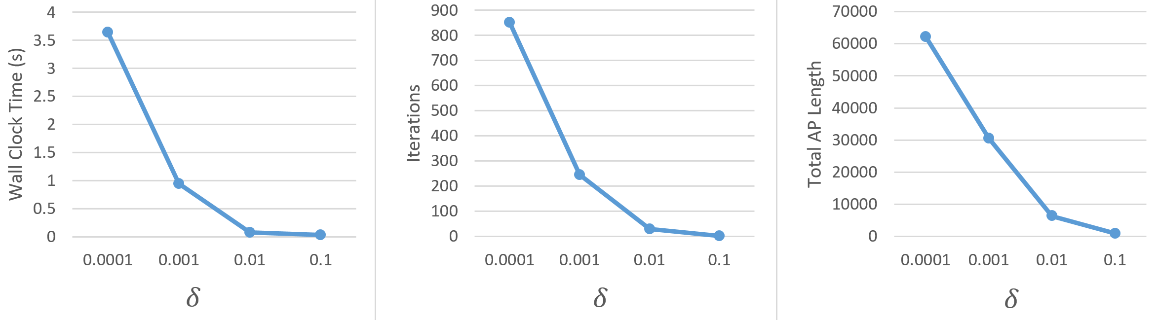
In the first set of tests, we compare the empirical performance of our algorithm to its theoretical analysis from Section 2. We execute $100$ runs, where each run executes our algorithm on a randomly selected pair of MNIST images for $\delta\in[0.0001,0.1]$. For each value of $\delta$, we record the wall-clock running time, iteration count, and total augmenting path length of our algorithm. These values, averaged over all runs, are plotted in Figure  1. We observe that the number of iterations is significantly less than the theoretical bound of roughly $\frac{2}{(1-\varepsilon)\delta}=4/\delta$. We also observe that the total augmenting path length is significantly smaller than the worst case bound of $n/\delta^{2}$ for even for the very small $\delta$ value of $0.0001$. This is because of two reasons. First, the inequality (8) (Proof of Lemma 2.4 in the supplement) used in bounding the augmenting path length is rarely tight; most augmenting paths have large slack with respect to this inequality. Second, to obtain the worst case bound, we assume that only one unit of flow is pushed through each augmenting path (see Proof of Lemma 2.4). However, in our experiments augmenting paths increased flow by a larger value whenever possible. As a result, we noticed that the total time taken by augmentations, even for the smallest value of $\delta$, was negligible and $\leq 2\%$ of the execution time.

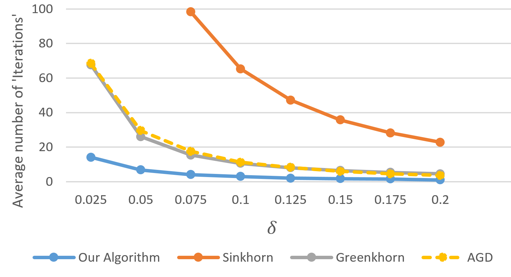
Next, we compare the number of iterations executed by our algorithm with the number of iterations executed by the Sinkhorn, Greenkhorn, and APDAGD algorithms. Here, by ‘iteration’ we refer to the the logical division of each algorithm into portions that take $\mathcal{O}(n^{2})$ time. For example, an iteration of the Greenkhorn algorithm corresponds to $n$ row/column updates. An iteration for our algorithm corresponds to a single phase. We execute 10 runs, where each run selects a random pair of MNIST images and executes all four algorithms using $\delta$ values in the range $[0.025,0.2]$.

Figure 2(a) depicts the average number of iterations for each algorithm. For the Sinkhorn, Greenkhorn and APDAGD algorithms, we see a significant increase in iterations as we choose smaller values of $\delta$. We believe this is because of numerical instability associated with these algorithms. Unlike these algorithms, our algorithm runs fairly quickly for very small values of $\delta$ (see Figure 1).

We repeat the test from Figure 2(a), and compare the average time taken to produce the result. The code for Greenkhorn and APDAGD are not optimized for actual running time, so we restrict to comparing our algorithm with the Sinkhorn algorithm, and record average wall-clock running time. The results of executing $100$ runs are plotted on the left in Figure 2(b). Under these conditions, we observe that the time taken by our algorithm is significantly less than that taken by the Sinkhorn algorithm. The cost of the solution produced by our algorithm, although within the error parameter $\delta$, was not always better than that of the cost of the solution produced by Sinkhorn. We repeat the same experimental setup, except with Sinkhorn receiving an error parameter of $5\delta$ while our algorithm continues to receive $\delta$. Our algorithm continues to have a better average execution time than Sinkhorn (plot on the right in Figure 2(b)). Moreover, we also observe that cost of solution produced by Sinkhorn is higher than the solution produced by our algorithm for every run across all values of $\delta$. In other words, for this experiment, our algorithm executed faster and produced a better quality solution than the Sinkhorn algorithm.

We presented an $\mathcal{O}(n^{2}(C/\delta)+n(C/\delta)^{2})$ time algorithm to compute a $\delta$-close approximation of the optimal transport. Our algorithm is an execution of a single scale of Gabow and Tarjan’s algorithm for appropriately scaled integer demands, supplies and costs. Our key technical contribution is a diameter sensitive analysis of the execution time of this algorithm.

In [29, Section 3.1, 3.2], it has been shown that the first and the second steps of our algorithm, i.e., Hungarian search and partial DFS, can be executed on a residual graph with costs $\overline{c}(\cdot,\cdot)$ in $\mathcal{O}(n\Phi(n)\log^{2}n)$ and $\mathcal{O}(n\Phi(n))$ time respectively; here $\Phi(n)$ is the query and update time of a dynamic weighted nearest neighbor data structure with respect to the cost function $c(\cdot,\cdot)$. Unlike in [29] where the costs, after scaling down by a factor $\delta^{\prime}$, are rounded up, $\overline{c}(\cdot,\cdot)$ is obtained by scaling down $c(\cdot,\cdot)$ by $\delta^{\prime}$, and is rounded down. This, however, does not affect the critical lemma [29, Lemma 3.2] and the result continues to hold. Several distances including the Euclidean distance and the squared-Euclidean distance admit such a dynamic weighted nearest neighbor data structure for planar point sets with poly-logarithmic query and update time [2, 16]. Therefore, we immediately obtain a $\tilde{\mathcal{O}}(n(C/\delta)^{2})$ time algorithm to compute a $\delta$-close approximation of the optimal transport for such distances. In [1, Section 4 (i)–(iii)], a similar link is made between an approximate nearest neighbor (ANN) data structure and a relative approximation algorithm.

The Sinkhorn algorithm scales well in parallel settings because the row and column update operations within each iteration can be easily parallelized. In the first step, our algorithm uses Dijkstra’s method that is inherently sequential. However, there is an alternate implementation of a single scale of Gabow and Tarjan’s algorithm that does not require Dijkstra’s search (see [19, Section 2.1]) and may be more amenable to parallel implementation. We conclude with the following open questions:

• •

  Can we design a combinatorial algorithm that uses approximate nearest neighbor data structure and produces a $\delta$-close transport plan for geometric costs in $\tilde{\mathcal{O}}(n(C/\delta)^{d})$ time?

• •

  Can we design a parallel combinatorial approximation algorithm that produces a $\delta$-close optimal transport for arbitrary costs?

Acknowledgements: Research presented in this paper was funded by NSF CCF-1909171. We would like to thank the anonymous reviewers for their useful feedback. All authors contributed equally to this research.

References

- Agarwal and Sharathkumar [2014] P. K. Agarwal and R. Sharathkumar. Approximation algorithms for bipartite matching with metric and geometric costs. In ACM Symposium on Theory of Computing, pages 555–564, 2014.
- Agarwal et al. [1999] P. K. Agarwal, A. Efrat, and M. Sharir. Vertical decomposition of shallow levels in 3-dimensional arrangements and its applications. SIAM J. Comput., 29(3):912–953, 1999.
- Altschuler et al. [2017] J. Altschuler, J. Weed, and P. Rigollet. Near-linear time approximation algorithms for optimal transport via sinkhorn iteration. In Neural Information Processing Systems, pages 1961–1971, 2017.
- Altschuler et al. [2018] J. Altschuler, F. Bach, A. Rudi, and J. Weed. Approximating the quadratic transportation metric in near-linear time. arxiv:1810.10046 [cs.DS], 2018.
- Arjovsky et al. [2017] M. Arjovsky, S. Chintala, and L. Bottou. Wasserstein GAN. arXiv:1701.07875v3 [stat.ML], 2017.
- Benamou et al. [2015] J.-D. Benamou, G. Carlier, M. Cuturi, L. Nenna, and G. Peyré. Iterative bregman projections for regularized transportation problems. SIAM Journal on Scientific Computing, 37(2):A1111–A1138, 2015.
- Bigot et al. [2017] J. Bigot, R. Gouet, T. Klein, A. López, et al. Geodesic PCA in the wasserstein space by convex PCA. In Annales de l’Institut Henri Poincaré, Probabilités et Statistiques, volume 53, pages 1–26. Institut Henri Poincaré, 2017.
- Blanchet et al. [2018] J. Blanchet, A. Jambulapati, C. Kent, and A. Sidford. Towards optimal running times for optimal transport. arXiv:1810.07717 [cs.DS], 2018.
- Cuturi [2013] M. Cuturi. Sinkhorn distances: Lightspeed computation of optimal transport. In Neural Information Processing Systems, pages 2292–2300, 2013.
- Cuturi and Doucet [2014] M. Cuturi and A. Doucet. Fast computation of wasserstein barycenters. In International Conference on Machine Learning, pages 685–693, 2014.
- Dvurechensky et al. [2018] P. Dvurechensky, A. Gasnikov, and A. Kroshnin. Computational optimal transport: Complexity by accelerated gradient descent is better than by sinkhorn’s algorithm. In International Conference on Machine Learning, pages 1366–1375, 2018.
- Edmonds and Karp [1972] J. Edmonds and R. M. Karp. Theoretical improvements in algorithmic efficiency for network flow problems. J. ACM, 19(2):248–264, 1972.
- Flamary et al. [2018] R. Flamary, M. Cuturi, N. Courty, and A. Rakotomamonjy. Wasserstein discriminant analysis. Machine Learning, 107(12):1923–1945, 2018.
- Gabow and Tarjan [1989] H. N. Gabow and R. Tarjan. Faster scaling algorithms for network problems. SIAM J. Comput., 18:1013–1036, October 1989.
- Jambulapati et al. [2019] A. Jambulapati, A. Sidford, and K. Tian. A direct iteration parallel algorithm for optimal transport. arxiv 1906.00618 [cs.DS], 2019.
- Kaplan et al. [2017] H. Kaplan, W. Mulzer, L. Roditty, P. Seiferth, and M. Sharir. Dynamic planar voronoi diagrams for general distance functions and their algorithmic applications. In ACM/SIAM Sympos. on Discrete Algorithms, pages 2495–2504, 2017.
- Khesin et al. [2019] A. B. Khesin, A. Nikolov, and D. Paramonov. Preconditioning for the geometric transportation problem. In Symposium on Computational Geometry, pages 15:1–15:14, 2019.
- Kuhn [1956] H. Kuhn. Variants of the hungarian method for assignment problems. Naval Research Logistics, 3(4):253–258, 1956.
- Lahn and Raghvendra [2019a] N. Lahn and S. Raghvendra. A faster algorithm for minimum-cost bipartite matching in minor-free graphs. In ACM/SIAM Sympos. on Discrete Algorithms, pages 569–588, 2019a.
- Lahn and Raghvendra [2019b] N. Lahn and S. Raghvendra. A weighted approach to the maximum cardinality bipartite matching problem with applications in geometric settings. In Symposium on Computational Geometry, pages 48:1–48:13, 2019b.
- Lee and Sidford [2014] Y. T. Lee and A. Sidford. Path finding methods for linear programming: Solving linear programs in (vrank) Iterations and Faster Algorithms for Maximum Flow. In IEEE Foundations of Computer Science, pages 424–433, 2014.
- Lin et al. [2019] T. Lin, N. Ho, and M. I. Jordan. On efficient optimal transport: An analysis of greedy and accelerated mirror descent algorithms. arXiv:1901.06482 [cs.DS], 2019.
- Mucha and Sankowski [2004] M. Mucha and P. Sankowski. Maximum matchings via gaussian elimination. In IEEE Foundations of Computer Science, pages 248–255, 2004.
- Phillips and Agarwal [2006] J. M. Phillips and P. K. Agarwal. On bipartite matching under the RMS distance. In Canadian Conference on Computational Geometry, 2006.
- Quanrud [2019] K. Quanrud. Approximating optimal transport with linear programs. In Symposium on Simplicity of Algorithms, volume 69, pages 6:1–6:9, 2019.
- Ramshaw and Tarjan [2012] L. Ramshaw and R. E. Tarjan. A weight-scaling algorithm for min-cost imperfect matchings in bipartite graphs. In IEEE Foundations of Computer Science, pages 581–590, 2012.
- Sandler and Lindenbaum [2011] R. Sandler and M. Lindenbaum. Nonnegative matrix factorization with earth mover’s distance metric for image analysis. IEEE Transactions on Pattern Analysis and Machine Intelligence, 33(8):1590–1602, 2011.
- Sharathkumar and Agarwal [2012a] R. Sharathkumar and P. K. Agarwal. A near-linear time approximation algorithm for geometric bipartite matching. In ACM Symposium on Theory of Computing, pages 385–394, 2012a.
- Sharathkumar and Agarwal [2012b] R. Sharathkumar and P. K. Agarwal. Algorithms for the transportation problem in geometric settings. In ACM/SIAM Sympos. on Discrete Algorithms, pages 306–317, 2012b.
- Sherman [2017] J. Sherman. Generalized preconditioning and undirected minimum-cost flow. In ACM/SIAM Sympos. on Discrete Algorithms, pages 772–780, 2017.
Appendix Supplement A Validity of the transport plan after augmentation
Note that the updated transport plan after each augmentation is valid. Augmenting along by the residual capacity will maintain a feasible flow and so, for any edge , . By our choice, is lower than the remaining demand at and the unused supply at . Therefore, after augmentation, the supplies transported to (resp. from ) increases by and remains at most (resp. ).
For any other demand (resp. supply) node (resp. ) with (resp. ), the total supplies transported to (resp. from ) after the transport plan is updated remains unchanged. This is because (resp. ) has exactly one forward and one backward edge of incident on it. The increase in supply transported to (resp. from ) via the forward edge is canceled out by the decrease in supply transported along the backward edge.
Appendix Supplement B Proof of Lemma 1.1
Proof.
To prove our claim, it suffices to construct a maximum transport plan for such that .
For any , we define . Note that the transport plan is not necessarily valid for . This is because the total flow of supplies from any supply node exceeds by
The third equality follows from the fact that is a maximum transport plan and so, . However, satisfies the demand constraints. Specifically, for any demand node , combining the facts that and we get,
To make a valid maximum transportation plan, for every supply node , we iteratively choose an edge incident on , say and reduce the flow of supplies along in and the excess supply , by . We continue this iterative process until reduces to . By repeating this iterative process for every supply node, will satisfy the supply constraints with equality and is a maximum transport plan for . Furthermore, since the supply transported in along the edge is at most
∎
Appendix Supplement C Proof of Lemma 2.1
First, without loss of generality, we transform and so that remains a -optimal transport plan and remains the minimum-cost maximum transport plan. Furthermore, this transformation guarantees that the dual weights for the -optimal transport plan are such that every edge for which the optimal transport plan has a positive flow, i.e., , also satisfies (3). We present this transformation next. If the dual weights for an edge do not satisfy (3), then its flow is . We reduce and by and also reduce the flow on the edge in to be and to . The transformed and continue to be -optimal transport plan and minimum cost maximum transport plan respectively for the new demands and supplies. Moreover, their difference in costs of and does not change due to this transformation and we are guaranteed that if the edge has a positive flow with respect to , i.e., then will satisfy (3). We present the rest of the proof assuming that and are transformed.
The weight of is