Counterpropagating continuous variable entangled states in lossy coupled-cavity optical waveguides
Abstract
We present an integrated source of counterpropagating entangled states based on a coupled resonator optical waveguide that is pumped by a classical pulsed source incident from above the waveguide. We investigate theoretically the generation and propagation of continuous variable entangled states in this coupled-cavity system in the presence of intrinsic loss. Using a tight-binding approximation, we derive analytic time-dependent expressions for the number of photons in each cavity, as well as for the correlation variance between the photons in different pairs of cavities, to evaluate the degree of quantum entanglement. We also derive simple approximate expressions for these quantities that can be used to guide the design of such systems, and discuss how pumping configurations and physical properties of the system affect the photon statistics and the degree of quantum correlation.
I Introduction
Entangled quantum states have potential applications in quantum teleportation ik Bouwmeester et al. - 1997/12/11/online; Jennewein et al. 2001, quantum computation, and quantum information Cerf et al. 2007; Bouwmeester et al. 2013. They can either involve discrete variables (DVs), such as the polarization of a photon, or continuous variables (CVs), such as the quadratures of a beam of light. Although DV systems provide high-fidelity operations, photonic-based DV entanglement is currently limited by the difficulties of single-photon generation and detection, and by high sensitivity to optical losses. In contrast, CV entanglement is more robust to loss, and can be more efficiently created and used for the implementation of quantum protocols Huang et al. 2016; Leverrier and Grangier 2011; Soh et al. 2015; Jia et al. 2004; Miwa et al. 2009. Spontaneous parametric down conversion (SPDC), a second order nonlinear process in which a pump photon is converted into a signal and an idler photon, is one of the processes that can be used to generate quantum correlated states U’Ren et al. 2006; Sciscione et al. 2006; Yang and Sipe 2007. It has been implemented in both bulk media and integrated photonic structures. However, as the size and complexity of quantum information processing systems increase, the limitations in achieving stability, precision, and small physical size with bulk optical systems become significant. Systems for on-chip SPDC, which are integrable with other photonic elements and could be used to generate CV entangled states involving two spatially separated sites, are therefore very promising Tan et al. 2011; Xiong et al. 2010; Tan and Zhang 2011.
One such platform involves the use of waveguides made of materials with a large second order nonlinear optical response, such as AlGaAs, to generate counterpropagating, quantum correlated photons Caillet et al. 2009; Orieux et al. 2011. The particular system we consider here is the coupled-resonator optical waveguide (CROW), in which the waveguide consists of optical cavities weakly coupled in one dimension. By adjusting the nature of the cavities and the coupling between them, the dispersive properties of the propagating modes can be controlled Yariv et al. 1999. Loss, which can destroy the nonclassical properties of light Slusher et al. 1985; Jasperse et al. 2011; Seifoory et al. 2017; Seifoory and Dignam 2018; Rai and Angelakis 2012, can also be controlled to some extent, allowing at least a partial optimization for particular applications. CROW structures have been shown to have potential in generating CV entangled states between two side cavities coupled to the CROW, and as well between spatially separated sites Tan et al. 2011. It is the latter application we study here.
Our integrated source of entangled states is schematically shown in Fig. 1. A pump pulse is incident on a set of central cavities from above. Consequently, in order for the phase matching condition to be fulfilled, the generated signal and idler modes propagate in opposite directions in the CROW structure. An important advantage of such a configuration is the absence of the pump mode in the guided direction. Moreover, it has also been shown that the properties of the counterpropagating guided signal and idler modes can be tuned using the spectral and spatial properties of the pump Orieux et al. 2011; Walton et al. 2003; Walton et al. 2004.

The tight-binding (TB) method Ashcroft and Mermin 2011; Fussell and Dignam 2007a, which uses localized single-cavity modes as a basis, can be applied to model the evolution of light in such a coupled structure. Assuming that all the cavities are identical and support the same mode with complex frequency , it has been shown com that in the nearest-neighbor tight-binding (NNTB) approximation the dispersion relation can be written as
| (1) |
where , , and are respectively the complex coupling parameter, the periodicity of the CROW, and the Bloch vector component. The imaginary part of the complex frequency is associated with the loss of the Bloch modes in the CROW. It is clear from Eq. (1) that these modes experience different loss rates; it has been shown that the rates can differ by an order of magnitude or more Kamandar Dezfouli 2015; Fussell and Dignam 2007b; Seifoory and Dignam 2018.
In our previous work, we focused on the time evolution of a state generated in a coupled-cavity system, and studied the evolution and propagation of squeezing and entanglement Seifoory and Dignam 2018. We presented analytic expressions for a general initial state, but only presented detailed results for an initial state that was a squeezed vacuum state in one of the cavities. In this work, we investigate both the generation and propagation of entangled states in coupled-cavity systems. In addition, we engineer the pump parameters to produce counterpropagating pulses of the generated signal and idler modes, which are entangled but are not individually squeezed. Including the effects of intrinsic propagation loss, we calculate the number of photons in each cavity and the CV correlation variance of photons in different cavities.
Previous approaches for generating counterpropagating entangled states have focused on photon pairs and been based either on ridge waveguides with vertical pumping Caillet et al. 2009; Orieux et al. 2011, or on periodic waveguides with horizontal pumping Saravi et al. 2017. The new approach of using a CROW has a number of advantages. First, the CROW allows us to control the group velocity and the frequency at which there is zero group velocity dispersion. Second, because a CROW can be modelled using a TB method, we are able to specify and model the effects of intrinsic scattering loss on the generated CV entanglement as a function of propagation distance, which is important for any application. Finally, using vertical pumping leads to counterpropagating entangled states, with no co-propagating pump at the outputs.
This paper is organized as follows. In Sec. II we present the general theory of the generation and the evolution of the generalized two mode squeezed state in lossy CROWs via SPDC. In Sec. III, we consider the special case of a pump that is Gaussian in time and space, and derive analytic expressions for the time dependence of the number of photons and the CV correlations. In Sec. IV, we present our results for a particular CROW in a slab photonic crystal, and discuss how they might be affected by the pumping configuration and the physical properties of the structure. Finally, in Sec. V, we present our conclusions.
II General Theory
In order to determine both the generation and evolution of the entangled squeezed states in the system, we divide the analysis into two separate tasks. First, we study the creation of the entangled photons via SPDC using the backward Heisenberg method Yang et al. 2008, which is intrinsically a lossless approach. Having determined the initial entangled states created by the pump, we then include the loss to see how the generated state evolves in time and how loss affects it. Note that this two-step approach is valid because, for the parameters considered in this paper, the pump pulse is short enough that the signal loss is negligible over its duration.
II.1 Generation
There are two mode types that are relevant here, the fundamental modes and the pump modes; we indicate them by and respectively. In the SPDC process, two photons are generated in modes from one pump photon in mode . Expanding the full displacement field in terms of the modes of interest, we have
| (2) |
where , , and are the modes, eigenfrequencies and annihilation operators of the pump field, respectively, and , , and are the corresponding quantities for the generated signal and idler fields. Note that the integral over in Eq. (2) and in the rest of the paper (except where explicitly noted) only ranges from to . The continuous index, , is to identify the different pump modes in 3D while identifies the polarization state. The normalization conditions for the modes are presented in Appendix A. Here
| (3) |
For convenience we put
| (4) |
and the linear Hamiltonian is then given by
| (5) |
where we neglect the zero point energy and use only the real part of for the mode frequency. The nonlinear Hamiltonian that should be added to to construct the full Hamiltonian is Yang et al. 2008
| (6) |
where is the coupling coefficient, which is given by
| (7) |
where is a real, position and frequency dependent refractive index and is the position-dependent second-order nonlinear susceptibility.
We take the pump to be a classical pulse incident on the slab, which we can expand as a superposition of the pump modes . We borrow a strategy from Yang et al. Yang et al. 2008 and define asymptotic-in and -out states to be respectively the input and output states of the nonlinear region at , taking to be the time when the pump is centred on the slab. For the asymptotic-in state that describes the classical pump pulse as a coherent state, we have
| (8) |
where is a complex number, and we normalize the complex function according to
| (9) |
The expectation value of the displacement field of the pump pulse is then
| (10) |
and since
| (11) |
we can identify as the expectation value of the number of photons in the pump pulse. Following the backward Heisenberg picture approach Yang et al. 2008, the asymptotic-out state for the generated photons in the first approximation is then
| (12) |
where is the biphoton wave function, which from Yang et al. Yang et al. 2008 is given by
| (13) |
where is a real and positive normalization constant chosen to ensure that .
While the biphoton wave function in general obeys the symmetry , it can sometimes be useful to work with a function that breaks this symmetry to focus attention on a particular quadrant of space. In this work, we will always choose the pump parameters such that to a very good approximation, is nonzero only when and have opposite signs, as we detail in Section III below. Then, we can write
| (14) |
We then define
| (15) |
where is the Heaviside function, such that we may rewrite Eq. (12) as
| (16) |
Employing a Schmidt decomposition Peres 2006; Ekert and Knight 1995, we have
| (17) |
for with , where the Schmidt functions are orthonormal,
| (18) |
We extend the sets of and associated with to form complete sets with
| (19) |
and with some of the appearing in Eq. (17) then equal to zero. Using Eqs. (16) and (17), the generated squeezed state can be written as
| (20) |
where the squeezing operator, , can be written as
| (21) |
where is the squeezing parameter,
| (22) |
and
| (23) |
Using Eq. (19), it can be shown that and .
The importance of the Schmidt decomposition and the operator transformation is that it enables us to express the generated state as a generalized two-mode squeezed state, where the modes are no longer the Bloch modes. As we shall see in the next section, this will enable us to easily determine the evolution of the state in the presence of loss.
II.2 Evolution
As mentioned earlier, we have assumed that the loss during the generation process is negligible. However, the effect of loss cannot be ignored when calculating the evolution of the generated pulses down the CROW.
Following the formalism presented in our previous work Seifoory and Dignam 2018 on lossy coupled-cavity systems, the individual single-mode cavity annihilation operator for the cavity, , can be written in terms of the mode annihilation operator of the coupled-cavity-system, , as
| (24) |
The time evolution of the full coupled-cavity annihilation operator can also be found by solving the adjoint master equation for this open, lossy system Breuer and Petruccione 2007. We have previously shown that the time dependence of the individual annihilation operators is given by
| (25) |
where is the corresponding operator in the Schrödinger representation Dignam and Dezfouli 2012. Using Eqs. (24), (25), and their complex conjugates, the time dependent average photon number in the cavity can be written as
| (26) |
where we have used the lossy dispersion relation of the CROW structure [Eq. (1)]. To facilitate the evaluation of , we introduce the restricted operators,
| (27) |
Using these operators, we can write
| (28) |
To evaluate each of these terms, we use the following Bogoliubov transformations
| (29) |
| (30) |
Using these in Eq. (28), we obtain
| (31) |
To study the degree of entanglement between the photons in cavities and in a CROW, we use the correlation variance, which is defined as
| (32) |
where
| (33) | ||||
It has been shown that can be considered as the inseparability criterion for entanglement Duan et al. 2000; Simon 2000; Masada et al. 2015; Zhang et al. 2015. Using Eq. (33) in Eq. (32), the time-dependent correlation variance can be written as
| (34) |
III Results for a Gaussian pump pulse
The results of the previous sections are general and independent of the temporal and spatial form of the pump pulse, as long as is nonzero only when and have opposite signs. However, in this section we consider the special case of a Gaussian pump pulse incident on the slab, and brought to a Gaussian focus there.
We assume that the slab does not have a significant effect on the pump pulse, and so take the pump modes to be plane waves in free space and set in Eq. (II.1). Thus, we have
| (35) |
where is the polarization unit vector. In what follows, we assume that in the vicinity of the CROW, the pump is polarized in the -direction. Thus, we obtain
| (36) |
where
| (37) |
is the Fourier transform of the transverse profile
| (38) |
and is the value of at which peaks. Here and are the radius of curvature and spot size, respectively, evaluated at and . We have assumed the Rayleigh range to be much larger than the slab thickness, which justifies the neglect of the Gouy phase. The prefactors have been chosen so that the normalization condition Eq. (9) becomes
| (39) |
Neglecting the dependence of the indices of refraction and the frequencies under the square root on , , and , based on the small frequency range of the input pump pulse and the limited range of the signal and idler photons in the CROW, we can rewrite the biphoton wave function of Eq. (15) as
| (40) |
Because we have made the approximation that the transverse profile of the pump does not depend on frequency (for the frequencies of interest) in Eq. (40) we set in the Dirac delta function.
We now employ the nearest-neighbour tight-binding approximation Fussell and Dignam 2007a and expand the modes in terms of the single-cavity quasimodes, , as
| (41) |
which leads to the lossy frequency dispersion given in Eq. (1). The single-cavity quasimodes and frequencies are calculated in the standard way using finite difference time domain calculations Fussell and Dignam 2007a. Assuming that the cavity modes are well-localized wel, we obtain
| (42) |
We define
| (43) |
and, because and spatial extent of the single-cavity quasimodes is small relative to that of the pump field, in the integral in Eq. (42) we replace by
| (44) |
to obtain the approximate expression
| (45) |
where
| (46) |
is the effective second order susceptibility for the system exp (See Appendix B for more details).
For , which we consider to be a real quantity at this point, Eq. (45) can be rewritten as
| (47) |
where
| (48) |

In order to derive analytic expressions for the photon number and correlation variance as a function of cavity index, , we need to place further restrictions on the pump pulse. From the first exponential in Eq. (47), we see that the biphoton wave function will only be non-negligible if is approximately equal to . Thus we set
| (49) | ||||
where the are small relative to , where is determined by the central frequency of the pump, through the equation
| (50) |
In order to obtain a biphoton wave function for which there is an analytic Schmidt decomposition, we take and choose the frequency width parameter, , of the pulse to satisfy , where . Now, expanding the cosines in Eq. (47) to first order in and , the biphoton wave function can be rewritten as
| (51) |
where
| (52) |
and
| (53) |
Strictly speaking, the biphoton wave function of Eq. (III) does not satisfy the restriction that it is zero unless and . However, as long as and are chosen to be small enough, then these conditions are satisfied to a very high degree. In what follows, we shall only consider situations where this is the case. Using the normalization condition, , it can be shown that
| (54) |
In Fig. 2, we plot three sample biphoton wave functions of the form given in Eq. (III) for different and for .
To graphically illustrate the validity of the assumptions made to obtain Eq. (III), in Fig. 3 we plot the dispersion of our CROW. The physical parameters of the CROW are from Ref. Fussell and Dignam 2007a. It consists of a dielectric slab of refractive index having a square array of cylindrical air voids of radius , height , and lattice vectors and , where is the period. The cavities are point defects formed by periodically removing air voids in a line with (see Fig. 1). The complex frequency, , and the complex coupling parameter, , of the structure are , and , respectively. To visualize the biphoton wave function superimposed on the CROW dispersion, we plot for and in Fig. 3 as well. As can be seen, the first order expansion of and about and is accurate as the dispersion within this range is very close to linear. In order for our Schmidt decomposition to be valid for this structure, and cannot be increased significantly beyond the chosen value of otherwise the biphoton wave function will not be confined to the quadrant where and . Note that increasing the pump width to higher values, , increases the accuracy of our approximation, as is evident from Figs. 2(b) and 2(c) where is and , respectively.

Before employing a Schmidt decomposition, we present the relation between and the temporal and spatial full width at half maximum (FWHM) of the pump pulse. Using Eqs. (38) and (53), the temporal FWHM of the pump can be written as
| (55) |
where is the time for a pulse with Bloch vector to travel one period. Similarly, using Eqs. (43) and (52), the spatial FWHM of the pump is found to be
| (56) |
Using these two equations, one can obtain a clear understanding of the necessary pumping conditions. For instance, the quantities considered in Fig. 2(a) correspond to a pump with and as the temporal and spatial FWHM, respectively. As we show later, for our CROW, the propagation loss in the system is very small while the squeezed light is being generated, which validates the neglect of loss during the generation process.
The special form of the biphoton wave function, Eq. (III), allows us to perform a Schmidt decomposition analytically U’Ren et al. 2003; Lvovsky et al. 2007; Blay et al. 2017 for as
| (57) |
where
| (58) |
| (59) |
and the are Hermite polynomials of order . Note that the Schmidt number is given by Zhukovsky et al. 2012
| (60) |
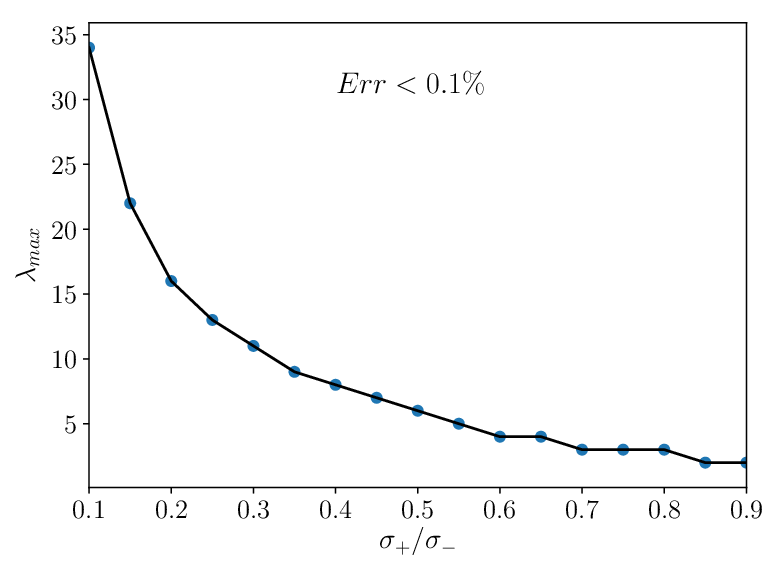
Using Eq. (58) for the special case where , it can be shown that the only nonzero term in Eq. (63) is for . However, in general, one needs to include several of the Schmidt modes (up to ) to accurately represent the biphoton wave function. To quantify the accuracy of the Schmidt decomposition used in our calculations, we define an error function as
| (61) |
where and are the exact and approximate expressions, respectively, given by Eq. (III) and
| (62) |
In Fig. 4 we plot the index of the maximum Schmidt mode needed to be included in , in order to ensure . For example, as can be seen, when , one needs to include terms () to achieve the desired accuracy.
Using these results in Eqs. (II.2) and (II.2), the time-dependent average photon number in the cavity is found to be
| (63) |
where
| (64) |
The time-dependent average photon number in the cavity when can be simplified to
| (65) |
We note that using Eq. (65) for a lossless system, one finds that the total number of photons in the CROW is , independent of , which agrees with the total number of generated photons in any two-mode squeezed state.
Following a procedure similar to that used to arrive at Eq. (63), one can derive the following expectation value for , which is needed in Eq. (34) to evaluate the variances of the quadrature operators and the correlation variance in the CROW structure:
| (66) |
Note that is simply the complex conjugate of Eq. (66).
In the next section, we will use these equations to determine the photon number and correlation variance under a variety of different pump conditions.
IV Results
Using the expectation values derived in Sec. III, we can now study the photon evolution and inseparability criteria for the generalized two-mode squeezed light inside the CROW structure. In Fig. 5, we plot the average number of photons in the th cavity for as a function of time for both a lossy (solid green line) and lossless (dashed grey line) system. The propagation of light between the coupled cavities and effect of loss on the number of photons in each cavity is evident in Figs. 5(a) and 5(b), where . Because the system and pump are spatially symmetric, the results are identical for . In Fig. 5(c), we plot the time-dependent average photon number in the th cavity with still, but with the and . As can be seen, the pulse width is wider for this smaller , as expected.
Since our input pump state is a coherent state, the number of pump photons is . We now examine what the pump parameters will be for a specific case of interest. We again consider the case where ; using Eqs. (55) and (56) this gives temporal and spatial FWHM for the pump of and , respectively. We choose the CROW material to be due to its high nonlinearity and relatively large bandgap. In addition, we choose the pump wavelength to be , which not only results in generating counterpropagating signal and idler photons at the telecommunication wavelength, , but also ensures operation below the band gap of . Choosing the periodicity of the CROW structure to yield a signal central wavelength of , gives . Using Eq. (46) and the normalization condition given in Appendix A, for our structure is approximately given by , where , appropriate for AlGaAs alloys Yang and Sipe 2007; Gili et al. 2016; Carletti et al. 2015, and at . We now seek to determine the approximate number of pump photons under the above conditions that will give a squeezing parameter of . Employing Eqs. (48) and (54), the average number of photons in the pump is found to be , which gives a total pump pulse energy of approximately . We note that all of the above pump characteristics are easily achievable from a Ti:Sapphire laser.

In Fig. 6 we plot the time-dependent correlation variances for different sets of lossy and lossless cavities in blue and grey, respectively. Note that there are fast oscillations that are not observable on this time scale. The dashed lines in the insets show the inseparability criteria below which the light is considered to be entangled. Here we only focus on cases where the two cavities considered are located the same distance from the central cavity, as this will yield the maximum entanglement; however, using Eq. (34) one can explore the entanglement between any two cavities of the CROW. As can be seen in Fig. 6(a) and (b), due to the loss in the system, the degree of entanglement decreases as the system evolves in time, whereas for a lossless system (the grey color) the degree of entanglement does not change as the light propagates.


In Fig. 7 we plot the maximum number of photons for a lossless and lossy CROW as a function of the cavity index, . As expected, when loss is included, the number of photons decreases as we move away from the central cavity. In Fig. 7 we also plot the minimum correlation variance for the lossless and lossy CROW as a function of cavity index, . As can be seen, due to the reduction in the number of photons in the lossy case, there is a decrease in the degree of entanglement as a function of . For instance, the minimum correlation variance at the tenth cavity is times the corresponding value at the one hundredth cavity.
For a general pump, the evolution equations for the photon number and correlation variance are quite complicated and it is difficult to discern the general behaviour or the effects of loss from the full equations. However, for the special case where and , approximate analytic expressions can be obtained. We begin by defining the complex quantity, , which enables us to rewrite as
| (67) |
Considering only the dominant terms in Eq. (65), to a very good approximation one can show that the time at which the photon number in the cavity peaks in a lossless system is . As can be seen in Fig. 5, the photon number peaks at essentially the same time in both lossy and lossless system. Using , we are able to derive the following approximate expression for the maximum photon number in the cavity (for ) in a lossy system:
| (68) |
Following the same procedure and using Eqs. (34) and (66), one obtains
| (69) |
We note first that both the photon number and the deviation of the correlation variance from depend linearly on . Thus, as expected, the separability is largest when the pump is short in time and narrow in space (for a fixed squeezing parameter, ). Now, according to Eqs. (68) and (69), under the above-mentioned pumping conditions the effect of loss on the maximum number of photons and on the entanglement as a function of is given by two exponential factors. The first factor accounts for the intrinsic loss in an individual cavity (which is also the intrinsic loss of the Bloch mode with ). The second factor accounts for the loss dispersion in the CROW, and results in a reduction in the loss. Of course, these analytic results are only valid when the effect of the dispersion of the loss is small.
We now consider how well these approximate expressions reproduce the exact results. In Fig. 7, we plot the results of Eqs. (68) and (69) with (black solid line) and without (red solid line) including the factor, . As can be seen, for this CROW the full approximate analytic expressions very accurately reproduces the exact results. Moreover, to a very good approximation, one can evaluate Eqs. (68) and (69) neglecting the loss-dispersion factor, . For example, for = and , the first and the second exponential factors in Eqs. (68) and (69) are and , respectively, showing that loss dispersion only changes the results by . In general, it can be shown that in order to have less than error in evaluating the photon number and the difference of the correlation variance from , the range of must be limited to .
Finally, we now consider the more general cases in which is not necessarily equal to . Under these conditions, we cannot derive simple expressions for the maximum photon number and entanglement as a function of . We present the results of the full calculations for a lossless system in Table 1 for a number of different pump durations and spatial widths; all other parameters are the same as in the previous plots. As can be seen, the maximum entanglement is obtained when the pump duration is as short as possible and the pump width is as narrow as possible (i.e. for our system).
We have also performed full calculations for the evolution in the presence of loss for different pump configurations. In Fig. 8, we compare the results of the full calculations with the results when the loss is incorporated approximately using only the exponential factor . We plot the maximum number of photons and the deviation of the minimum of the correlation variance from the inseparability threshold of 4 for a lossy system as a function of for different pumping configurations. As can be seen, for short distances from the central cavity (small ), the effect of loss on the result can, to a very good approximation, still be explained by only including the exponential factor . However, for the cavities far from the central cavity (large ), although the general trends can still be predicted by such an approximation, the difference between the exact and approximation results becomes pronounced and the validity of this approximation becomes questionable. In order to show the difference between exact and approximate results for large , in Fig. 9 we plot the relative difference between the results from the full calculations and those from approximating the loss in the system by only considering the exponential factor as a function of , for and . As expected, when , we obtain a relative error of approximately , which is simply due to the dispersion factor, . However, in general, the error depends on , and is different for the photon number and correlation variance, due to the different way in which loss dispersion affects these two quantities. As can be seen in this specific example, evaluating using the approximation method results in a deviation from the results of the full calculations when , while, the relative difference for the maximum number of photons is always less than . It is thus evident that a simple exponential factor will capture the general effect of loss on the correlation, but it may not be very accurate depending on the structure and the pump conditions.
| 1.23 | 2.24 | 0.77 | 2.51 | 3.74 | |
| 0.38 | 0.44 | 0.58 | 0.65 | 0.74 |


V Conclusion
In this work we studied the generation and propagation of entangled states in lossy coupled-cavity systems. We applied the tight-binding method to evaluate the fields and complex frequencies for the leaky modes of lossy coupled-cavity system, and presented analytic time-dependent expressions for the photon number and correlation variance in a lossy CROW structure. We showed how properties such as the average number of photons in each cavity and the correlations between cavities are affected by loss. For the CROW structure considered in this work, we found that as the light gets far from the central cavity, the effects of loss become more significant and cannot be ignored. Moreover, we obtained simple, approximate analytic expressions for the effects of loss on the propagation of the generated light in the CROW, and have shown that they can be used to predict general trends. However, depending on the details of the pumping conditions and the CROW structure itself, the accuracy of this approximation varies, and to get an accurate result, specifically for cavities far from the central cavity, the effect of loss cannot be well-described using a simple exponential factor that is given by the loss in an individual cavity. Using full numerical results is suggested for optimization. Yet these analytic results allow researchers to easily explore the spectral and spatial pumping configurations needed to generate the counterpropagating entangled states in a CROW.
Appendix A
In this appendix we present the normalization condition for the modes. Considering the refractive index of the material to be nondispersive within the range of frequency considered here, following Yang et al. Yang et al. 2008, the normalization conditions can be written as
| (70) |
and
| (71) |
Using Eq. (41) in Eq. (70) we obtain the normalization condition for the single-cavity modes as
| (72) |
Appendix B
In this appendix we present an accurate approximate analytic result for the summation in Eq. (42). Starting from Eq. (42) we have
| (73) |
Approximating this sum as an integral, we obtain
| (74) |
where and . Now using
| (75) |
we can write
| (76) |
One can show numerically that for , the approximation made here is accurate to within
References
- ik Bouwmeester et al. (- 1997/12/11/online) D. ik Bouwmeester, J. ian-W. ei Pan, K. laus Mattle, M. anfred Eibl, H. arald Weinfurter, and A. nton Zeilinger, “- Experimental quantum teleportation,” - 390, – – (- 1997/12/11/online).
- Jennewein et al. (2001) Thomas Jennewein, Gregor Weihs, Jian-Wei Pan, and Anton Zeilinger, “Experimental nonlocality proof of quantum teleportation and entanglement swapping,” Phys. Rev. Lett. 88, 017903 (2001).
- Cerf et al. (2007) N.J. Cerf, N.J. Cerf, G. Leuchs, and E.S. Polzik, Quantum Information with Continuous Variables of Atoms and Light (Imperial College Press, 2007).
- Bouwmeester et al. (2013) D. Bouwmeester, A.K. Ekert, and A. Zeilinger, The Physics of Quantum Information: Quantum Cryptography, Quantum Teleportation, Quantum Computation (Springer Berlin Heidelberg, 2013).
- Huang et al. (2016) Duan Huang, Peng Huang, Dakai Lin, and Guihua Zeng, “Long-distance continuous-variable quantum key distribution by controlling excess noise,” Scientific Reports 6, 19201 EP – (2016), article.
- Leverrier and Grangier (2011) Anthony Leverrier and Philippe Grangier, “Continuous-variable quantum-key-distribution protocols with a non-gaussian modulation,” Phys. Rev. A 83, 042312 (2011).
- Soh et al. (2015) Daniel B. S. Soh, Constantin Brif, Patrick J. Coles, Norbert Lütkenhaus, Ryan M. Camacho, Junji Urayama, and Mohan Sarovar, “Self-referenced continuous-variable quantum key distribution protocol,” Phys. Rev. X 5, 041010 (2015).
- Jia et al. (2004) Xiaojun Jia, Xiaolong Su, Qing Pan, Jiangrui Gao, Changde Xie, and Kunchi Peng, “Experimental demonstration of unconditional entanglement swapping for continuous variables,” Phys. Rev. Lett. 93, 250503 (2004).
- Miwa et al. (2009) Yoshichika Miwa, Jun-ichi Yoshikawa, Peter van Loock, and Akira Furusawa, “Demonstration of a universal one-way quantum quadratic phase gate,” Phys. Rev. A 80, 050303 (2009).
- U’Ren et al. (2006) Alfred B. U’Ren, Reinhard K. Erdmann, Manuel de la Cruz-Gutierrez, and Ian A. Walmsley, “Generation of two-photon states with an arbitrary degree of entanglement via nonlinear crystal superlattices,” Phys. Rev. Lett. 97, 223602 (2006).
- Sciscione et al. (2006) L. Sciscione, M. Centini, C. Sibilia, M. Bertolotti, and M. Scalora, “Entangled, guided photon generation in -dimensional photonic crystals,” Phys. Rev. A 74, 013815 (2006).
- Yang and Sipe (2007) Zhenshan Yang and J. E. Sipe, “Generating entangled photons via enhanced spontaneous parametric downconversion in algaas microring resonators,” Opt. Lett. 32, 3296–3298 (2007).
- Tan et al. (2011) Hua-Tang Tan, Wei-Min Zhang, and Gao-xiang Li, “Entangling two distant nanocavities via a waveguide,” Phys. Rev. A 83, 062310 (2011).
- Xiong et al. (2010) Heng-Na Xiong, Wei-Min Zhang, Xiaoguang Wang, and Meng-Hsiu Wu, “Exact non-markovian cavity dynamics strongly coupled to a reservoir,” Phys. Rev. A 82, 012105 (2010).
- Tan and Zhang (2011) Hua-Tang Tan and Wei-Min Zhang, “Non-markovian dynamics of an open quantum system with initial system-reservoir correlations: A nanocavity coupled to a coupled-resonator optical waveguide,” Phys. Rev. A 83, 032102 (2011).
- Caillet et al. (2009) X. Caillet, V. Berger, G. Leo, and S. Ducci, “A semiconductor source of counterpropagating twin photons: a versatile device allowing the control of the two-photon state,” Journal of Modern Optics 56, 232–239 (2009), https://doi.org/10.1080/09500340802192431 .
- Orieux et al. (2011) Adeline Orieux, Xavier Caillet, Aristide Lemaître, Pascal Filloux, Ivan Favero, Giuseppe Leo, and Sara Ducci, “Efficient parametric generation of counterpropagating two-photon states,” J. Opt. Soc. Am. B 28, 45–51 (2011).
- Yariv et al. (1999) Amnon Yariv, Yong Xu, Reginald K. Lee, and Axel Scherer, “Coupled-resonator optical waveguide:?a proposal and analysis,” Opt. Lett. 24, 711–713 (1999).
- Slusher et al. (1985) R. E. Slusher, L. W. Hollberg, B. Yurke, J. C. Mertz, and J. F. Valley, “Observation of squeezed states generated by four-wave mixing in an optical cavity,” Phys. Rev. Lett. 55, 2409–2412 (1985).
- Jasperse et al. (2011) M. Jasperse, L. D. Turner, and R. E. Scholten, “Relative intensity squeezing by four-wave mixing with loss: an analytic model and experimental diagnostic,” Opt. Express 19, 3765–3774 (2011).
- Seifoory et al. (2017) Hossein Seifoory, Sean Doutre, Marc. M. Dignam, and J. E. Sipe, “Squeezed thermal states: the result of parametric down conversion in lossy cavities,” J. Opt. Soc. Am. B 34, 1587–1596 (2017).
- Seifoory and Dignam (2018) Hossein Seifoory and Marc M. Dignam, “Squeezed-state evolution and entanglement in lossy coupled-resonator optical waveguides,” Phys. Rev. A 97, 023840 (2018).
- Rai and Angelakis (2012) Amit Rai and Dimitris G. Angelakis, “Dynamics of nonclassical light in integrated nonlinear waveguide arrays and generation of robust continuous-variable entanglement,” Phys. Rev. A 85, 052330 (2012).
- Walton et al. (2003) Zachary D. Walton, Mark C. Booth, Alexander V. Sergienko, Bahaa E. A. Saleh, and Malvin C. Teich, “Controllable frequency entanglement via auto-phase-matched spontaneous parametric down-conversion,” Phys. Rev. A 67, 053810 (2003).
- Walton et al. (2004) Zachary D. Walton, Alexander V. Sergienko, Bahaa E. A. Saleh, and Malvin C. Teich, “Generation of polarization-entangled photon pairs with arbitrary joint spectrum,” Phys. Rev. A 70, 052317 (2004).
- Ashcroft and Mermin (2011) N.W. Ashcroft and N.D. Mermin, Solid State Physics (Cengage Learning, 2011).
- Fussell and Dignam (2007a) David P. Fussell and Marc M. Dignam, “Engineering the quality factors of coupled-cavity modes in photonic crystal slabs,” Applied Physics Letters 90, 183121 (2007a), http://dx.doi.org/10.1063/1.2737430 .
- (28) Throughout this work, we place a tilde on top of quantities that are inherently complex (as opposed to real).
- Kamandar Dezfouli (2015) Mohsen Kamandar Dezfouli, Quantum Nonlinear Optics in Lossy Coupled-Cavities in Photonic Crystal Slabs, Ph.D. thesis, Queen’s University (2015).
- Fussell and Dignam (2007b) David P. Fussell and Marc M. Dignam, “Spontaneous emission in coupled microcavity-waveguide structures at the band edge,” Opt. Lett. 32, 1527–1529 (2007b).
- Saravi et al. (2017) Sina Saravi, Thomas Pertsch, and Frank Setzpfandt, “Generation of counterpropagating path-entangled photon pairs in a single periodic waveguide,” Phys. Rev. Lett. 118, 183603 (2017).
- Yang et al. (2008) Zhenshan Yang, Marco Liscidini, and J. E. Sipe, “Spontaneous parametric down-conversion in waveguides: A backward heisenberg picture approach,” Phys. Rev. A 77, 033808 (2008).
- Peres (2006) A. Peres, Quantum Theory: Concepts and Methods, Fundamental Theories of Physics (Springer Netherlands, 2006).
- Ekert and Knight (1995) Artur Ekert and Peter L. Knight, “Entangled quantum systems and the schmidt decomposition,” American Journal of Physics 63, 415–423 (1995), https://doi.org/10.1119/1.17904 .
- Breuer and Petruccione (2007) H. P. Breuer and F. Petruccione, The theory of open quantum systems (Oxford University Press, 2007).
- Dignam and Dezfouli (2012) Marc. M. Dignam and Mohsen Kamandar Dezfouli, “Photon–quantum-dot dynamics in coupled-cavity photonic crystal slabs,” Phys. Rev. A 85, 013809 (2012).
- Duan et al. (2000) Lu-Ming Duan, G. Giedke, J. I. Cirac, and P. Zoller, “Inseparability criterion for continuous variable systems,” Phys. Rev. Lett. 84, 2722–2725 (2000).
- Simon (2000) R. Simon, “Peres-horodecki separability criterion for continuous variable systems,” Phys. Rev. Lett. 84, 2726–2729 (2000).
- Masada et al. (2015) Genta Masada, Kazunori Miyata, Alberto Politi, Toshikazu Hashimoto, Jeremy L. O’Brien, and Akira Furusawa, “Continuous-variable entanglement on a chip,” Nat Photon 9, 316–319 (2015), letter.
- Zhang et al. (2015) Yun Zhang, Ryuhi Okubo, Mayumi Hirano, Yujiro Eto, and Takuya Hirano, “Experimental realization of spatially separated entanglement with continuous variables using laser pulse trains,” Scientific Reports 5, 13029 EP – (2015), article.
- (41) By well-localized we mean that the integral would be negligible unless both of these modes are at the same .
- (42) For the range of pump frequency considered in this paper, to a very good approximation one can consider .
- U’Ren et al. (2003) A. B. U’Ren, K. Banaszek, and I. A. Walmsley, “Photon engineering for quantum information processing,” Quantum Info. Comput. 3, 480–502 (2003).
- Lvovsky et al. (2007) A. I. Lvovsky, Wojciech Wasilewski, and Konrad Banaszek, “Decomposing a pulsed optical parametric amplifier into independent squeezers,” Journal of Modern Optics 54, 721–733 (2007), https://doi.org/10.1080/09500340600777805 .
- Blay et al. (2017) Daniel R. Blay, M. J. Steel, and L. G. Helt, “Effects of filtering on the purity of heralded single photons from parametric sources,” Phys. Rev. A 96, 053842 (2017).
- Zhukovsky et al. (2012) Sergei V. Zhukovsky, Lukas G. Helt, Payam Abolghasem, Dongpeng Kang, John E. Sipe, and Amr S. Helmy, “Bragg reflection waveguides as integrated sources of entangled photon pairs,” J. Opt. Soc. Am. B 29, 2516–2523 (2012).
- Gili et al. (2016) V. F. Gili, L. Carletti, A. Locatelli, D. Rocco, M. Finazzi, L. Ghirardini, I. Favero, C. Gomez, A. Lemaître, M. Celebrano, C. De Angelis, and G. Leo, “Monolithic algaas second-harmonic nanoantennas,” Opt. Express 24, 15965–15971 (2016).
- Carletti et al. (2015) L. Carletti, A. Locatelli, O. Stepanenko, G. Leo, and C. De Angelis, “Enhanced second-harmonic generation from magnetic resonance in algaas nanoantennas,” Opt. Express 23, 26544–26550 (2015).