跳到论文正文
W Papers独立论文阅读器 arXiv:1905.11477 论文正文 计算阅读时间 · 0%
引用这篇论文根据当前论文元数据生成,正式投稿前建议核对。


License: arXiv.org perpetual non-exclusive license
arXiv:1905.11477v1 [eess.SY] 27 May 2019

Multi-sensor State Estimation over Lossy Channels using Coded Measurements

Tianju Sui Email: suitj@mail.dlut.edu.cn    Damian Marelli*cor Email: Damian.Marelli@newcastle.edu.au    Ximing Sun Email: sunxm@dlut.edu.cn    Minyue Fu Email: minyue.fu@newcastle.edu.au
Abstract

This paper focuses on a networked state estimation problem for a spatially large linear system with a distributed array of sensors, each of which offers partial state measurements, and the transmission is lossy. We propose a measurement coding scheme with two goals. Firstly, it permits adjusting the communication requirements by controlling the dimension of the vector transmitted by each sensor to the central estimator. Secondly, for a given communication requirement, the scheme is optimal, within the family of linear causal coders, in the sense that the weakest channel condition is required to guarantee the stability of the estimator. For this coding scheme, we derive the minimum mean-square error (MMSE) state estimator, and state a necessary and sufficient condition with a trivial gap, for its stability. We also derive a sufficient but easily verifiable stability condition, and quantify the advantage offered by the proposed coding scheme. Finally, simulations results are presented to confirm our claims.

keywords
Networked state estimation, Sensor fusion, Packet loss, Minimum mean-square error.
††corresponding: [††address: School of Control Science and Engineering, Dalian University of Technology, Dalian, China.††address: School of Automation, Guangdong University of Technology, Guangzhou, China.††address: French Argentine International Center for Information and Systems Sciences, National Scientific and Technical Research Council, Argentina.††address: School of Electrical Engineering and Computer Science, The University of Newcastle, NSW 2308, Australia.††thanks: This work was not presented at any conference.

, , ,

cor]Corresponding author.

1 Introduction

This work is concerned with the sensor fusion problem over lossy channels. Each sensor obtains a partial state measurement subject to some additive noise, and transmits it to a remote (central) estimator through a communication network involving packet loss. The estimator computes a minimum mean-square error (MMSE) estimate of the system state using the received measurements. The configuration is illustrated in Fig. 1. This setup is motivated by a wide range of applications including networked control systems, multi-agent systems, smart electricity networks and sensor networks [1, 2].

Refer to caption
Figure 1: Networked state estimation using raw measurements.

The problem of networked state estimation, based on MMSE estimation, has received significant attention in recent years [3, 4, 5, 6]. One of the major difficulties comes from the packet loss occurring while transmitting sensor measurements. A central problem consists in determining the packet loss statistics required to guarantee the stability of the MMSE estimator. This was done in [3] for the case in which the packet loss is independent and identically distributed. This result has been generalized to different packet loss models and algebraic system’s structure in [7, 8, 9, 10, 11, 12, 13, 14]. The most general result within this line was recently reported in [15], where the authors state a conceptional necessary and sufficient condition with a trivial gap, for general packet loss statistics and system structure.

The above works assume that raw measurements without preprocessing are transmitted to the estimator. It turns out that the use of preprocessing can relax the channel requirements, in terms of channel statistics, needed to guarantee stability [16, 17]. For example, in [18], the sensor locally obtains a MMSE estimate and transmits it instead of its measurement. A drawback of this approach is that this increases the amount of communications, because the estimated state needs to be transmitted, which typically has a higher dimension than the raw measurement. To rectify this, a coded measurement [19, 20] is built by using a linear combination of the most recent measurements within a coding window, and this is transmitted instead of the raw measurement [21, 22].

The works described so far consider the case in which a single sensor transmits over a single channel. In many applications, the system whose state needs to be estimated covers a wide geographical area. Such a large-scale system is typically equipped with multiple sensors for measurements. The state estimation problem resulting from this setup has been studied in a number of works [23, 24, 25, 26, 27, 28, 29]. In a sensor network setup, all the sensors can transmit their measurements to a central estimator over different channels, each with its own packet loss statistics. Conditions for guaranteeing stability in this network setup can be very complex, and may be very strong for certain systems, as reported in [26, 27, 28, 30].

In [15], the authors derived a necessary and sufficient condition, having a trivial gap, for the stability of a MMSE estimator. These condition is stated in very general terms, so it can be applied in a wide range of settings. In the present work, we make use of this result to design a MMSE estimator for a multi-sensor network problem. Our contributions are the following: (1) In the context of this work, the stability of the estimator depends on how reliable are the communication channels between each sensor and the estimator. We propose a coding scheme that, while reducing the amount of transmitted data, i.e., the dimension of the coded vector transmitted by each sensor at each time step, achieves the weakest requirement on the channel reliability required to guarantee stability. (2) While the aforementioned condition is necessary and sufficient, its computation can be mathematically involved is some cases. To go around this, we also provide a sufficient condition for easier computation. (3) We quantify the gain, in terms of channel reliability, offered by the proposed coding scheme, when compared with the scheme using raw measurements.

The rest of the paper is organized as follows. In Section 2 we describe the system, channel and coding models. In Section 3, we derive the expression of the state estimator using coded measurements. In Section 4.1 we provide a necessary and sufficient condition with a trivial gap for the stability of the MMSE estimator. In Section 4.2 we derive a simpler sufficient condition for its stability. In Section 5 we derive a necessary and sufficient condition with a trivial gap for the stability of the MMSE estimator using raw measurements, and quantify the advantage offered by the proposed coding scheme. We give simulation results illustrating our claims in Section 6, and give concluding remarks in Section 7. To improve readability, some proofs are given in the Appendix.

Notation \thethm

The sets of real and natural numbers are denoted by ℝ\mathbb{R} and ℕ\mathbb{N}, respectively. We use ℙ⁡(𝒮)\mathbb{P}(\mathcal{S}) to denote the probability of the set 𝒮\mathcal{S} and 𝔼⁡(x)\mathbb{E}(x) to denote the expected value of the random variable xx. For a vector or matrix xx we use x⊤x^{\top} to denote its transpose. We use IdI_{d} to denote the dd-dimensional identity matrix and II to denote the same matrix when the dimension is clear from the context.

2 Problem statement

Consider a discrete-time stochastic system

xt+1=A​xt+wt,x_{t+1}=Ax_{t}+w_{t}, (1)

where xt∈ℝnx_{t}\in\mathbb{R}^{n} is the system state and wt∼𝒩⁡(0,Q)w_{t}\sim\mathcal{N}\left(0,Q\right) is white Gaussian noise with Q≥0Q\geq 0. The initial time is t0t_{0} and the initial state is xt0∼𝒩⁡(x¯t0,Pt0)x_{t_{0}}\sim\mathcal{N}\left(\bar{x}_{t_{0}},P_{t_{0}}\right), with Pt0≥0P_{t_{0}}\geq 0. A sensor network with II nodes, as depicted in Fig. 1, is used to measure the state in a distributed manner. For each i∈{1,⋯,I}i\in\{1,\cdots,I\}, the measurement yti∈ℝmiy_{t}^{i}\in\mathbb{R}^{m_{i}} obtained at sensor ii is given by

yti=Ci​xt+vti,y_{t}^{i}=C^{i}x_{t}+v_{t}^{i}, (2)

where vti∼𝒩⁡(0,Ri)v_{t}^{i}\sim\mathcal{N}\left(0,R^{i}\right) is mim_{i}-dimensional white Gaussian noise with Ri>0R^{i}>0. Let m=∑i=1Imim=\sum_{i=1}^{I}m_{i} and C⊤=[C1⊤,⋯,CI⊤]∈ℝn×mC^{\top}=\left[C^{1\top},\cdots,C^{I\top}\right]\in\mathbb{R}^{n\times m}. We assume that (A,C)(A,C) is detectable and x0,wt,vtix_{0},w_{t},v_{t}^{i} are jointly independent.

We are concerned with a networked estimation system, where each sensor is linked to the central estimator through a communication network. Due to the channel unreliability, the transmitted packets may be randomly lost. We use a binary random process γti\gamma_{t}^{i} to describe the packet loss process. That is, γti=1\gamma_{t}^{i}=1 indicates that the packet from sensor ii is successfully delivered to the estimator at time tt, and γti=0\gamma_{t}^{i}=0 indicates that the packet is lost. We assume that the random variables γti\gamma_{t}^{i}, t∈ℕt\in\mathbb{N}, i∈{1,⋯,I}i\in\{1,\cdots,I\} are independent and identically distributed (i.i.d). Also, for each i∈{1,…,I}i\in\left\{1,\ldots,I\right\}, pi=𝔼⁡[γti]p_{i}=\mathbb{E}\left[\gamma_{t}^{i}\right].

As a consequence of packet loss, the estimator may fail to generate a stable state estimate. To improve the stability, instead of transmitting the raw measurements from each sensor, we encode them before transmission, as depicted in Fig 2. More precisely, for a given coding window length L∈ℕL\in\mathbb{N}, the coded measurement of sensor ii at time tt, after going through the channel, is given by

zti=∑l=1Lγti​Ht,li⊤​yt−l+1i∈ℝci,z_{t}^{i}=\sum_{l=1}^{L}\gamma_{t}^{i}H_{t,l}^{i\top}y_{t-l+1}^{i}\in\mathbb{R}^{c_{i}}, (3)

for some coding weight matrices Ht,li∈ℝci×miH_{t,l}^{i}\in\mathbb{R}^{c_{i}\times m_{i}}, l∈{1,⋯,L}l\in\{1,\cdots,L\}, with ci≤mic_{i}\leq m_{i}, and the convention that yt=0y_{t}=0 for t≤t0t\leq t_{0}.

Refer to caption
Figure 2: Networked state estimation using coded sensor measurements.
Remark 1.

The coding scheme described in (3) allows reducing the dimension of the transmitted information from mim_{i} to cic_{i}, to the extent to which even a scalar (ci=1c_{i}=1) can be transmitted. This obviously reduce the communication load. We will show in Section 5 that the coding scheme can improve the stability of the state estimator with any choice of 1≤ci≤mi1\leq c_{i}\leq m_{i}.

To represent the packet loss process for all sensors at time tt, we introduce

Γt\displaystyle\Gamma_{t} =diag⁡{Γt1,⋯,ΓtI}∈𝔻,\displaystyle=\mathrm{diag}\left\{\Gamma_{t}^{1},\cdots,\Gamma_{t}^{I}\right\}\in\mathbb{D},
Γti\displaystyle\Gamma_{t}^{i} =γti​Ici,\displaystyle=\gamma_{t}^{i}I_{c_{i}},

where 𝔻\mathbb{D} consists of the 2I2^{I} matrices resulting from all possible values of γti\gamma_{t}^{i}. The information available to the estimator from time t0t_{0} to tt is then given by

ℱt0,t={(Γt0,Γt0​zt0),⋯,(Γt,Γt​zt)},\mathcal{F}_{t_{0},t}=\left\{\left(\Gamma_{t_{0}},\Gamma_{t_{0}}z_{t_{0}}\right),\cdots,\left(\Gamma_{t},\Gamma_{t}z_{t}\right)\right\},

where zt⊤=[zt1⊤,⋯,ztI⊤]z_{t}^{\top}=\left[z_{t}^{1\top},\cdots,z_{t}^{I\top}\right]. Using this information, the MMSE estimator computes

x^t|t−1​(ℱt0,t)=𝔼⁡[xt|ℱt0,t].\hat{x}_{t|t-1}\left(\mathcal{F}_{t_{0},t}\right)=\mathbb{E}\left[x_{t}|\mathcal{F}_{t_{0},t}\right].

Its prediction error covariance is defined by

Pt|t−1​(ℱt0,t)=𝔼⁡[(xt−x^t|t−1)​(xt−x^t|t−1)⊤|ℱt0,t].P_{t|t-1}\left(\mathcal{F}_{t_{0},t}\right)=\mathbb{E}\left[\left(x_{t}-\hat{x}_{t|t-1}\right)\left(x_{t}-\hat{x}_{t|t-1}\right)^{\top}|\mathcal{F}_{t_{0},t}\right].
Definition 2.

We say that the estimator is stable if [3]

supt0∈ℤPt0≥0lim supt→∞‖𝔼⁡(Pt+1|t​(ℱt0,t))‖<∞.\sup_{\begin{subarray}{c}t_{0}\in\mathbb{Z}\\ P_{t_{0}}\geq 0\end{subarray}}\limsup_{t\rightarrow\infty}\left\|\mathbb{E}\left(P_{t+1|t}\left(\mathcal{F}_{t_{0},t}\right)\right)\right\|<\infty.

As it is known [3, 18, 14], when the spectral radius of AA is greater than one, the packet loss can lead to an unstable estimator. Our goal is to design LL and HtH_{t}, t∈ℕt\in\mathbb{N}, to make the stability condition as weak as possible. In doing so, we also provide expressions for x^t|t−1\hat{x}_{t|t-1} and Pt|t−1P_{t|t-1}. Notice that, to simplify the notation, we use x^t|t−1\hat{x}_{t|t-1} and Pt|t−1P_{t|t-1} in place of x^t|t−1​(ℱt0,t)\hat{x}_{t|t-1}\left(\mathcal{F}_{t_{0},t}\right) and Pt|t−1​(ℱt0,t)P_{t|t-1}\left(\mathcal{F}_{t_{0},t}\right). We will use this notation in the rest of the paper.

3 The MMSE state estimation

In this section we assume that LL and Ht,liH_{t,l}^{i}, ∀t,l,i\forall t,l,i are given, and derive the expressions of x^t|t−1\hat{x}_{t|t-1} and Pt|t−1P_{t|t-1}.

Recall that C⊤=[C1⊤,⋯,CI⊤]∈ℝn×mC^{\top}=\left[C^{1\top},\cdots,C^{I\top}\right]\in\mathbb{R}^{n\times m} and define yt⊤=[yt1⊤,⋯,ytI⊤]∈ℝ1×my_{t}^{\top}=\left[y_{t}^{1\top},\cdots,y_{t}^{I\top}\right]\in\mathbb{R}^{1\times m} and vt⊤=[vt1⊤,⋯,vtI⊤]∈ℝ1×mv_{t}^{\top}=\left[v_{t}^{1\top},\cdots,v_{t}^{I\top}\right]\in\mathbb{R}^{1\times m}. We can then rewrite (2) as

yt\displaystyle y_{t} =C​xt+vt.\displaystyle=Cx_{t}+v_{t}.

Let c=∑i=1Icic=\sum_{i=1}^{I}c_{i}, Ht,l=diag⁡(Ht,l1⋯Ht,lI)∈ℝc×mH_{t,l}=\mathrm{diag}\left(\begin{array}[]{ccc}H_{t,l}^{1}&\cdots&H_{t,l}^{I}\end{array}\right)\in\mathbb{R}^{c\times m} and Ht=[Ht,1,⋯,Ht,L]∈ℝc×m​LH_{t}=\left[H_{t,1},\cdots,H_{t,L}\right]\in\mathbb{R}^{c\times mL}. Let also Γti=γti​Ici\Gamma_{t}^{i}=\gamma_{t}^{i}I_{c_{i}} and Γt=diag⁡{Γt1,⋯,ΓtI}\Gamma_{t}=\mathrm{diag}\left\{\Gamma_{t}^{1},\cdots,\Gamma_{t}^{I}\right\}, and recall that zt⊤=[zt1⊤,⋯,ztI⊤]∈ℝ1×cz_{t}^{\top}=\left[z_{t}^{1\top},\cdots,z_{t}^{I\top}\right]\in\mathbb{R}^{1\times c}. We can then rewrite (3) as

zt=Γt​Ht​[yt⊤,⋯,yt−L+1⊤]⊤.z_{t}=\Gamma_{t}H_{t}\left[y_{t}^{\top},\cdots,y_{t-L+1}^{\top}\right]^{\top}.

Let ut⊤=[xt⊤,yt⊤,⋯,yt−L+1⊤]∈ℝ1×(n+m​L)u_{t}^{\top}=\left[x_{t}^{\top},y_{t}^{\top},\cdots,y_{t-L+1}^{\top}\right]\in\mathbb{R}^{1\times(n+mL)}. We can obtain a state-space representation of (3) as follows

ut+1\displaystyle u_{t+1} =A¯​ut+ϵt,\displaystyle=\bar{A}u_{t}+\epsilon_{t}, (4)
zt\displaystyle z_{t} =D¯t​ut,\displaystyle=\bar{D}_{t}u_{t}, (5)

where

A¯\displaystyle\bar{A} =[A00C​A000I0],ϵt=[wtC​wt+vt+10],\displaystyle=\left[\begin{array}[]{ccc}A&0&0\\ CA&0&0\\ 0&I&0\end{array}\right],\quad\epsilon_{t}=\left[\begin{array}[]{c}w_{t}\\ Cw_{t}+v_{t+1}\\ 0\end{array}\right],
D¯t\displaystyle\bar{D}_{t} =Γt​[0Ht]=[D¯t1,⋯,D¯tI].\displaystyle=\Gamma_{t}\left[\begin{array}[]{cc}0&H_{t}\end{array}\right]=\left[\bar{D}_{t}^{1},\cdots,\bar{D}_{t}^{I}\right].

Thus, the expressions of x^t|t−1\hat{x}_{t|t-1} and Pt|t−1P_{t|t-1} can be derived by running a Kalman filter[31, 3] on (4)-(5). The resulting estimator is given by the following recursions

x^t|t−1\displaystyle\hat{x}_{t|t-1} =[I,0]​u^t|t−1,\displaystyle=\left[I,0\right]\hat{u}_{t|t-1},
Pt|t−1\displaystyle P_{t|t-1} =[I,0]​Σt|t−1​[I,0]⊤,\displaystyle=\left[I,0\right]\Sigma_{t|t-1}\left[I,0\right]^{\top},

where

u^t+1|t\displaystyle\hat{u}_{t+1|t} =A¯​u^t|t,\displaystyle=\bar{A}\hat{u}_{t|t},
u^t|t\displaystyle\hat{u}_{t|t} =u^t|t−1+∑i=1Iγki​Kti​(zti−D¯ti​u^t|t−1),\displaystyle=\hat{u}_{t|t-1}+\sum_{i=1}^{I}\gamma_{k}^{i}K_{t}^{i}\left(z_{t}^{i}-\bar{D}_{t}^{i}\hat{u}_{t|t-1}\right),
Σt+1|t\displaystyle\Sigma_{t+1|t} =A¯​Σt|t​A¯⊤+Q¯,\displaystyle=\bar{A}\Sigma_{t|t}\bar{A}^{\top}+\bar{Q},
Σt|t\displaystyle\Sigma_{t|t} =(I−∑i=1Iγki​Kti​D¯ti)​Σt|t−1,\displaystyle=\left(I-\sum_{i=1}^{I}\gamma_{k}^{i}K_{t}^{i}\bar{D}_{t}^{i}\right)\Sigma_{t|t-1},

with

Kti\displaystyle K_{t}^{i} =Σt|t−1​D¯i⊤​(D¯i​Σt|t−1​D¯i⊤)†,\displaystyle=\Sigma_{t|t-1}\bar{D}^{i\top}\left(\bar{D}^{i}\Sigma_{t|t-1}\bar{D}^{i\top}\right)^{\dagger},
Q¯\displaystyle\bar{Q} =[QQ​C⊤0C​QC​Q​C⊤+R0000],\displaystyle=\left[\begin{array}[]{ccc}Q&QC^{\top}&0\\ CQ&CQC^{\top}+R&0\\ 0&0&0\end{array}\right],

and initialized by

u^t0+1|t0=0,Σt0+1|t0=[Pt0Pt0​D¯t0⊤0D¯t0​Pt0D¯t0​Pt0​D¯t0⊤0000].\hat{u}_{t_{0}+1|t_{0}}=0,\quad\Sigma_{t_{0}+1|t_{0}}=\left[\begin{array}[]{ccc}P_{t_{0}}&P_{t_{0}}\bar{D}_{t_{0}}^{\top}&0\\ \bar{D}_{t_{0}}P_{t_{0}}&\bar{D}_{t_{0}}P_{t_{0}}\bar{D}_{t_{0}}^{\top}&0\\ 0&0&0\end{array}\right].

4 Stability Analysis for the MMSE estimator

In this section we provide conditions for the stability of the MMSE estimator derived in Section 3. In Section 4.1 we provide a necessary and sufficient condition with a trivial gap, and give the values of the design parameters LL and HtH_{t}, t∈ℕt\in\mathbb{N}, making this condition as weak as possible. In Section 4.2 we provide a sufficient condition for stability which is easier to verify.

4.1 Necessary and sufficient condition

In this section we state a necessary and sufficient condition, having a trivial gap, for the stability of the MMSE estimator using coded measurements. We then design LL and HtH_{t}, t∈ℕt\in\mathbb{N} to make this condition as weak as possible.

Let A¯=T¯​J¯​T¯−1\bar{A}=\bar{T}\bar{J}\bar{T}^{-1} be the Jordan normal form of A¯\bar{A}. We can then write (4)-(5) in Jordan canonical form as

u~t+1\displaystyle\tilde{u}_{t+1} =J¯​u~t+ϵ~t,\displaystyle=\bar{J}\tilde{u}_{t}+\tilde{\epsilon}_{t}, (6)
zt\displaystyle z_{t} =D~t​u~t,\displaystyle=\tilde{D}_{t}\tilde{u}_{t}, (7)

where u~t=T¯−1​ut\tilde{u}_{t}=\bar{T}^{-1}u_{t}, ϵ~t=T¯−1​ϵt\tilde{\epsilon}_{t}=\bar{T}^{-1}\epsilon_{t} and D~t=D¯t​T¯\tilde{D}_{t}=\bar{D}_{t}\bar{T}.

Lemma 3.

Let A=T​J​T−1A=TJT^{-1} be the Jordan normal form of AA. Then

J¯=diag⁡(J,Z1,⋯,ZL),\bar{J}=\mathrm{diag}\left(J,Z_{1},\cdots,Z_{L}\right), (8)

where ZlZ_{l}, l∈{1,⋯,L}l\in\left\{1,\cdots,L\right\} are mm-dimensional Jordan blocks with zero eigenvalues, and there exist matrices UU and VV such that

T¯=[T0UV].\bar{T}=\left[\begin{array}[]{cc}T&0\\ U&V\end{array}\right]. (9)
PROOF.

Let t¯=[0,v⊤]⊤\bar{t}=\left[0,v^{\top}\right]^{\top} with v⊤=[v1⊤,⋯,vL⊤]v^{\top}=\left[v_{1}^{\top},\cdots,v_{L}^{\top}\right]. We then have

A¯​t¯=A¯​[0,v⊤]⊤=[0,0,v1⊤,⋯,vL−1⊤]⊤.\bar{A}\bar{t}=\bar{A}\left[0,v^{\top}\right]^{\top}=\left[0,0,v_{1}^{\top},\cdots,v_{L-1}^{\top}\right]^{\top}.

It follows that A¯\bar{A} has mm generalized eigenvectors of rank LL with zero associated eigenvalue. Now, suppose that tt is an eigenvector of AA with eigenvalue λ\lambda. Let

t¯=[t⊤,(C​t)⊤,λ−1​(C​t)⊤,…,λ−L+2​(C​t)⊤]⊤\bar{t}=\left[t^{\top},(Ct)^{\top},\lambda^{-1}(Ct)^{\top},\ldots,\lambda^{-L+2}(Ct)^{\top}\right]^{\top}

It is straightforward to show that A¯​t¯=λ​t¯\bar{A}\bar{t}=\lambda\bar{t}. Hence, t¯\bar{t} is an eigenvector of A¯\bar{A} with eigenvalue λ\lambda. Using a similar but somehow more tedious argument, we can show that, for any generalized eigenvector tt of AA, there will be a generalized eigenvector t¯\bar{t} of A¯\bar{A}, with the same order and eigenvalue. Hence, the whole set of generalized eigenvectors of A¯\bar{A} is formed by either t¯=[0,v⊤]⊤\bar{t}=\left[0,v^{\top}\right]^{\top} for some vv or t¯=[t⊤,u⊤]⊤\bar{t}=\left[t^{\top},u^{\top}\right]^{\top}, for some uu and tt being a generalized eigenvector of AA. Thus, (9) follows. Also, the first nn eigenvalues of A¯\bar{A} equal those of AA, and the remaining are all zero. Hence, (8) follows.

Definition 4.

A set of complex numbers xi∈ℂx_{i}\in\mathbb{C}, i=1,⋯,Ii=1,\cdots,I, is said to have a common finite multiplicative order ι∈ℕ\iota\in\mathbb{N} up to a constant a∈ℂa\in\mathbb{C}, if xiι=aιx_{i}^{\iota}=a^{\iota}, for all i=1,⋯,Ii=1,\cdots,I. If there do not exist ι\iota and aa satisfying the above, the set is said not to have common finite multiplicative order.11 1 For example, eπ2​ȷe^{\frac{\pi}{2}\jmath} and eπ​ȷe^{{\pi}\jmath} have a common finite multiplicative order for that (eπ2​ȷ)4=(eπ​ȷ)4=1(e^{\frac{\pi}{2}\jmath})^{4}=(e^{{\pi}\jmath})^{4}=1. While, eπ2​ȷe^{\frac{\pi}{\sqrt{2}}\jmath} and eπ​ȷe^{{\pi}\jmath} do not have a common finite multiplicative order since there does not exist k∈ℕk\in\mathbb{N} such that (eπ2​ȷ)k=(eπ​ȷ)k=1(e^{\frac{\pi}{\sqrt{2}}\jmath})^{k}=(e^{{\pi}\jmath})^{k}=1.

It is straightforward to see that there is a unique partition of JJ in diagonal blocks of the form

J=diag⁡(J1,⋯,JK),J=\mathrm{diag}\left(J_{1},\cdots,J_{K}\right), (10)

such that, for every k=1,…,Kk=1,\ldots,K, the diagonal entries of the sub-matrices JkJ_{k} have a common finite multiplicative order ιk\iota_{k} up to aka_{k}, and for any k≠lk\neq l, the diagonal entries of the matrix diag⁡(Jk,Jl)\mathrm{diag}(J_{k},J_{l}) do not have common finite multiplicative order. Let dkd_{k} denote the dimension of JkJ_{k} and aka_{k} its magnitude. For each t∈ℕt\in\mathbb{N}, let

D~t=[D~t,1,⋯,D~t,K,D~t,∗],\tilde{D}_{t}=\left[\tilde{D}_{t,1},\cdots,\tilde{D}_{t,K},\tilde{D}_{t,\ast}\right],

be the partition of D~t\tilde{D}_{t} defined such that, for every k=1,…,Kk=1,\ldots,K, the number of columns of D~t,k\tilde{D}_{t,k} equals the dimension of JkJ_{k}. Let

Ot,T,k=[D~t,k​Jkt⋮D~t+T−1,k​Jkt+T−1].O_{t,T,k}=\left[\begin{array}[]{c}\tilde{D}_{t,k}J_{k}^{t}\\ \vdots\\ \tilde{D}_{t+T-1,k}J_{k}^{t+T-1}\end{array}\right].

Our next step is to state a necessary and sufficient condition for the stability of (6)-(7). To this end, we aim to use the result in [15, Theorem 14]. This result is stated under assumptions which are very general, but technically involved. Fortunately, we have a way around this technical difficulty. We have that {D~t:t∈ℕ}\{\tilde{D}_{t}:t\in\mathbb{N}\} is a sequence of random matrices, with discrete distribution, such that {D~t:t∈ℕ}\{\tilde{D}_{t}:t\in\mathbb{N}\} is a statistically independent set, and whose statistics are cyclostationary with period MM. Hence, it follows from [15, Proposition 18] that the conditions for [15, Theorem 14] are guaranteed. Also, these conditions consider all FMO blocks of (6)-(7). In view of Lemma 3, this system has K+1K+1 blocks. However, the eigenvalue of the last FMO block equals zero. Hence, the conditions need only consider the first KK blocks. We then obtain the following result.

Theorem 5.

(Combination of [15, Proposition 18] and [15, Theorem 14]) Suppose that the sequence of coding matrices {Ht:t∈ℕ}\{H_{t}:t\in\mathbb{N}\} is PP-periodic, i.e., Ht+P=HtH_{t+P}=H_{t}, for all t∈ℕt\in\mathbb{N}. Then, the MMSE estimator using coded measurements is stable if

max1≤k≤K⁡|ak|2​Φk<1,\max_{1\leq k\leq K}|a_{k}|^{2}\Phi_{k}<1,

and unstable if

max1≤k≤K⁡|ak|2​Φk>1,\max_{1\leq k\leq K}|a_{k}|^{2}\Phi_{k}>1,

where the channel unreliability measure Φk\Phi_{k} with respect to block kk is defined by

Φk=max⁡lim supT→∞0≤t<M⁡ℙ​(Ot,T,k​ does not have FCR)1/T,\Phi_{k}=\max_{0\leq t<M}\limsup_{T\rightarrow\infty}\mathbb{P}\left(O_{t,T,k}\text{ does not have FCR}\right)^{1/T},

and MM is the least common multiple of PP and ιk\iota_{k}, k∈{1,⋯,K}k\in\left\{1,\cdots,K\right\}.

Remark 6.

The result above is inconclusive for the case of max1≤k≤K⁡|ak|2​Φk=1\max_{1\leq k\leq K}|a_{k}|^{2}\Phi_{k}=1. For this reason, we say that the necessary and sufficient condition in Theorem 5 has a trivial gap.

In order to evaluate the condition in Theorem 5, we need to compute the channel unreliability measure Φk\Phi_{k} with respect to each block kk. This measure depends on the design parameters LL and HtH_{t}, t∈ℕt\in\mathbb{N}. Our next goal is to provide an expression of Φk\Phi_{k}, together with the choices of LL and HtH_{t}, t∈ℕt\in\mathbb{N}, so that we can minimize Φk\Phi_{k}.

The measure Φk\Phi_{k} is defined in terms of the probability that the matrix Ot,T,kO_{t,T,k} does not have full column rank (FCR). Our first step towards the computation of Φk\Phi_{k} is to replace Ot,T,kO_{t,T,k} by a different matrix, which we denote by O~t,T,k\tilde{O}_{t,T,k}, for which the aforementioned probability is easier to compute.

For each i∈{1,⋯,I}i\in\left\{1,\cdots,I\right\}, let C~i=Ci​T\tilde{C}^{i}=C^{i}T and

C~i=[C~1i,⋯,C~Ki],\tilde{C}^{i}=\left[\tilde{C}_{1}^{i},\cdots,\tilde{C}_{K}^{i}\right], (11)

be the partition of C~i\tilde{C}^{i} defined such that, for every k=1,…,Kk=1,\ldots,K, the number of columns of C~ki\tilde{C}_{k}^{i} equals the dimension of JkJ_{k}. Let Hti=[Ht,1i,⋯,Ht,Li]H_{t}^{i}=\left[H_{t,1}^{i},\cdots,H_{t,L}^{i}\right] and define, for each k∈{1,⋯,K}k\in\left\{1,\cdots,K\right\} and t,T∈ℕt,T\in\mathbb{N}, the following matrix

O~t,T,k\displaystyle\tilde{O}_{t,T,k} =[O~t,T,k1⋮O~t,T,kI],withO~t,T,ki=[o~k,ti⋮o~k,t+T−1i],\displaystyle=\left[\begin{array}[]{c}\tilde{O}_{t,T,k}^{1}\\ \vdots\\ \tilde{O}_{t,T,k}^{I}\end{array}\right],\qquad\text{with}\qquad\tilde{O}_{t,T,k}^{i}=\left[\begin{array}[]{c}\tilde{o}_{k,t}^{i}\\ \vdots\\ \tilde{o}_{k,t+T-1}^{i}\end{array}\right],
o~k,ti\displaystyle\tilde{o}_{k,t}^{i} =Γti​Hti​Gki​Jkt,andGki=[C~ki⋮C~ki​Jk−L+1].\displaystyle=\Gamma_{t}^{i}H_{t}^{i}G_{k}^{i}J_{k}^{t},\qquad\text{and}\qquad G_{k}^{i}=\left[\begin{array}[]{c}\tilde{C}_{k}^{i}\\ \vdots\\ \tilde{C}_{k}^{i}J_{k}^{-L+1}\end{array}\right].

We have the following result.

Lemma 7.

For each k∈{1,⋯,K}k\in\{1,\cdots,K\},

Φk=max⁡lim supT→∞0≤t<M⁡ℙ​(O~t,T,k​ does not have FCR)1/T.\Phi_{k}=\max_{0\leq t<M}\limsup_{T\rightarrow\infty}\mathbb{P}\left(\tilde{O}_{t,T,k}\text{ does not have FCR}\right)^{1/T}.
PROOF.

See Appendix A.

Our next step is to use Lemma 7 to provide an expression for Φk\Phi_{k}, together with the choices of LL and HtH_{t}, t∈ℕt\in\mathbb{N}, minimizing its value.

Recall that the packet arrival at time tt is represented by the diagonal matrix Γt\Gamma_{t}. Let 𝔻\mathbb{D} denote the set of all possible values of Γt\Gamma_{t}. We use Γt,T={Γt,⋯,Γt+T−1}∈𝔻T\Gamma_{t,T}=\left\{\Gamma_{t},\cdots,\Gamma_{t+T-1}\right\}\in\mathbb{D}^{T} to represent the packet arrivals in the past-time horizon of length TT starting from tt. For given packet-arrival pattern S∈𝔻MS\in\mathbb{D}^{M}, we use νi​(S)\nu^{i}(S) to denote the number of measurements from node ii included in SS.

Let 𝒢ki\mathcal{G}_{k}^{i} denote the row span of

Ωki=[Gki⋮Gki​Jkdk−1].\Omega_{k}^{i}=\left[\begin{array}[]{c}G_{k}^{i}\\ \vdots\\ G_{k}^{i}J_{k}^{d_{k}-1}\end{array}\right]. (12)
Definition 8.

We say that set ℒ⊆{1,⋯,I}\mathcal{L}\subseteq\left\{1,\cdots,I\right\} of nodes is insufficient for block kk if

span⁡(⋃i∈ℒ𝒢ki)≠ℝdk.\mathrm{span}\left(\bigcup_{i\in\mathcal{L}}\mathcal{G}_{k}^{i}\right)\neq\mathbb{R}^{d_{k}}.

An insufficient set ℒ\mathcal{L} is maximal if either ℒ={1,⋯,I}\mathcal{L}=\left\{1,\cdots,I\right\} or, for all i∉ℒi\notin\mathcal{L}, the set ℒ∪{i}\mathcal{L}\cup\{i\} is not insufficient. Let 𝕃k\mathbb{L}_{k} denote the collection of all maximal insufficient sets for block kk.

Recall that cic_{i} is the dimension of zkiz_{k}^{i}. For each ℒ∈𝕃k\mathcal{L}\in\mathbb{L}_{k}, we say that a set of measurement counts ℳ={0≤Mi≤M:i∉ℒ}\mathcal{M}=\left\{0\leq M^{i}\leq M:i\notin\mathcal{L}\right\} is insufficient for ℒ\mathcal{L} and kk if, for any choice of ci​Mic_{i}M^{i} vectors vji∈𝒢kiv_{j}^{i}\in\mathcal{G}_{k}^{i}, i∉ℒi\notin\mathcal{L}, j∈{1,⋯,ci​Mi}j\in\{1,\cdots,c_{i}M^{i}\}, we have

span⁡(⋃i∈ℒ𝒢ki∪⋃i≠ℒj∈{1,⋯,ci​Mi}vji)≠ℝdk.\mathrm{span}\left(\bigcup_{i\in\mathcal{L}}\mathcal{G}_{k}^{i}\cup\bigcup_{\begin{subarray}{c}i\neq\mathcal{L}\\ j\in\{1,\cdots,c_{i}M^{i}\}\end{subarray}}v_{j}^{i}\right)\neq\mathbb{R}^{d_{k}}. (13)

An insufficient set of counts ℳ={0≤Mi≤M:i∉ℒ}\mathcal{M}=\left\{0\leq M^{i}\leq M:i\notin\mathcal{L}\right\} is maximal if for any i∉ℒi\notin\mathcal{L} for which Mi<MM^{i}<M, the set obtained by replacing MiM^{i} by Mi+1M^{i}+1 is not insufficient. Let 𝕄k​(ℒ)\mathbb{M}_{k}\left(\mathcal{\mathcal{L}}\right) denote the collection of all maximal insufficient sets of counts for ℒ\mathcal{L} and kk. Recall that pi=𝔼⁡[γti]p_{i}=\mathbb{E}\left[\gamma_{t}^{i}\right], i∈{1,⋯,I}i\in\{1,\cdots,I\}, denotes the packet receival rate for sensor ii. We have the following result.

Assumption 9

The sequence of coding matrices {Ht:t∈ℕ}\{H_{t}:t\in\mathbb{N}\} is PP-periodic and generated using a pseudo-random sequence with absolutely continuous distribution.

Theorem 10.

Under Assumption 9, if L≥dkL\geq d_{k} for all k∈{1,⋯,K}k\in\{1,\cdots,K\}, then w.p.11 over the random outcomes of HtH_{t}, the resulting value of Φk\Phi_{k} is minimized w.r.t. LL and HtH_{t}, t∈ℕt\in\mathbb{N}. Furthermore, its value is

Φk=maxℒ∈𝕃k⁡max⁡∏i∉ℒℳ∈𝕄k​(ℒ)⁡(1−pi)1−MiM,\Phi_{k}=\max_{\mathcal{L}\in\mathbb{L}_{k}}\max_{\mathcal{M}\in\mathbb{M}_{k}(\mathcal{L})}\prod_{i\notin\mathcal{L}}\left(1-p_{i}\right)^{1-\frac{M^{i}}{M}}, (14)

where MM is the least common multiple of PP and ιk\iota_{k} for any k∈{1,⋯,K}k\in\left\{1,\cdots,K\right\}.

PROOF.

See Appendix B.

Remark 11.

We point out that, while Theorem 10 asserts that the coding matrix design the stated in Assumption 9 is optimal for the purpose of estimator stability, the same design may not be optimal for the purpose of minimizing the estimation error covariance.

Remark 12.

For a given FMO block k∈{1,⋯,K}k\in\{1,\cdots,K\}, maximal insufficient set ℒ∈𝕃k\mathcal{L}\in\mathbb{L}_{k} and node i∉ℒi\notin\mathcal{L}, the vectors vjiv_{j}^{i}, j∈{1,⋯,ci​Mi}j\in\{1,\cdots,c_{i}M^{i}\} belong to the subspace 𝒢ki⊂ℝdk\mathcal{G}_{k}^{i}\subset\mathbb{R}^{d_{k}}. Suppose that the FMO block kk is observable, i.e., span⁡(⋃i=1I𝒢ki)=ℝdk\mathrm{span}\left(\bigcup_{i=1}^{I}\mathcal{G}_{k}^{i}\right)=\mathbb{R}^{d_{k}}. Let ℳ={0≤Mi≤M:i∉ℒ}∈𝕄k​(ℒ)\mathcal{M}=\left\{0\leq M^{i}\leq M:i\notin\mathcal{L}\right\}\in\mathbb{M}_{k}(\mathcal{L}) be a maximal insufficient set of counts for ℒ\mathcal{L}. Then, since (13) needs to hold for any choice of vjiv_{j}^{i}’s, it follows that an increment in the dimension cic_{i} of the data transmitted by sensor ii would lead to a reduction of the measurement count MiM^{i} for that sensor. In view of 14, this will in turn reduce Φk\Phi_{k}. Hence, there is a tradeoff between the communication load (i.e., the value of cic_{i} for all i∈{1,⋯,Ii\in\{1,\cdots,I}) and the robustness to packet losses (i.e., the value of Φk\Phi_{k}).

The above expression of Φk\Phi_{k} greatly simplifies in the limit case as the period PP of the pseudo-random sequence used to generate HtH_{t}, t∈ℕt\in\mathbb{N} tends to infinity. This is stated in the following corollary of Theorem 10. This result represents most practical situations, as periods of pseudo-random sequences are typically very large.

Corollary 13.

Under the assumptions of Theorem 10,

limP→∞Φk=max⁡∏i∉ℒℒ∈𝕃k⁡(1−pi).\lim_{P\rightarrow\infty}\Phi_{k}=\max_{\mathcal{L}\in\mathbb{L}_{k}}\prod_{i\notin\mathcal{L}}\left(1-p_{i}\right). (15)
PROOF.

Notice that, in view of the choices of LL and HtH_{t}, if rank⁡(O~t,T,ki)<rank⁡(Gki),\mathrm{rank}\left(\tilde{O}_{t,T,k}^{i}\right)<\mathrm{rank}\left(G_{k}^{i}\right), then every new measurement from node ii yields rank⁡(O~t,T+1,ki)≥rank⁡(O~t,T,ki)+1\mathrm{rank}\left(\tilde{O}_{t,T+1,k}^{i}\right)\geq\mathrm{rank}\left(\tilde{O}_{t,T,k}^{i}\right)+1. Hence, for any ℒ∈𝕃k\mathcal{L}\in\mathbb{L}_{k} and ℳ∈𝕄k​(ℒ)\mathcal{M}\in\mathbb{M}_{k}(\mathcal{L}), we must have that Mi<rank⁡(Gki)M^{i}<\mathrm{rank}\left(G_{k}^{i}\right), for all i∉ℒi\notin\mathcal{L}. Since MM tends to infinity as so does PP, we have

limP→∞Φk\displaystyle\lim_{P\rightarrow\infty}\Phi_{k} =limP→∞maxℒ∈𝕃k⁡max⁡∏i∉ℒℳ∈𝕄k​(ℒ)⁡(1−pi)1−MiM\displaystyle=\lim_{P\rightarrow\infty}\max_{\mathcal{L}\in\mathbb{L}_{k}}\max_{\mathcal{M}\in\mathbb{M}_{k}(\mathcal{L})}\prod_{i\notin\mathcal{L}}\left(1-p_{i}\right)^{1-\frac{M^{i}}{M}}
=maxℒ∈𝕃k⁡max⁡∏i∉ℒℳ∈𝕄k​(ℒ)⁡(1−pi)\displaystyle=\max_{\mathcal{L}\in\mathbb{L}_{k}}\max_{\mathcal{M}\in\mathbb{M}_{k}(\mathcal{L})}\prod_{i\notin\mathcal{L}}\left(1-p_{i}\right)
=max⁡∏i∉ℒℒ∈𝕃k⁡(1−pi).\displaystyle=\max_{\mathcal{L}\in\mathbb{L}_{k}}\prod_{i\notin\mathcal{L}}\left(1-p_{i}\right).
Remark 14.

The above Corollary 13 shows that, when the period PP of the pseudo-random sequence used to generate coding matrices is sufficiently large, the stability condition is no longer affected by the dimension cic_{i} of coded measurements. Nevertheless, a larger value of cic_{i} is still helpful to improve the accuracy of the estimation.

4.2 An easily verifiable sufficient condition

The necessary and sufficient condition stated in Theorem 10 requires splitting the system in KK blocks. In this section we derive a condition which is only sufficient, but simpler to compute as it does not require the aforementioned splitting.

Let

Ξk\displaystyle\Xi_{k} =[Γ(k−1)​P​H(k−1)​P​F⋮Γk​P−1​Hk​P−1​F​AP−1],\displaystyle=\left[\begin{array}[]{c}\Gamma_{(k-1)P}H_{(k-1)P}F\\ \vdots\\ \Gamma_{kP-1}H_{kP-1}FA^{P-1}\end{array}\right],

with

F=[C⋮C​AL−1].F=\left[\begin{array}[]{c}C\\ \vdots\\ CA^{L-1}\end{array}\right].

We have the following result.

Lemma 15.

If Ξk\Xi_{k} does not have full column rank,

Pk​P|k​P−1≤ρ​(A)2​P​ρ​(A)2ρ​(A)2−1​P(k−1)​P|(k−1)​P−1,P_{kP|kP-1}\leq\rho(A)^{2P}\frac{\rho(A)^{2}}{\rho(A)^{2}-1}P_{(k-1)P|(k-1)P-1}, (16)

where ρ⁡(A)\rho\left(A\right) denotes the spectral radius of AA. If Ξk\Xi_{k} has full column rank, there exists 0<P¯∈ℝn×n0<\bar{P}\in\mathbb{R}^{n\times n} independent of P(k−1)​P|(k−1)​P−1P_{(k-1)P|(k-1)P-1}, such that

Pk​P|k​P−1≤P¯.P_{kP|kP-1}\leq\bar{P}. (17)
PROOF.

See Appendix C.

For each i∈{1,⋯,I}i\in\{1,\cdots,I\}, let

Fi=[Ci⋮Ci​AL−1].F^{i}=\left[\begin{array}[]{c}C^{i}\\ \vdots\\ C^{i}A^{L-1}\end{array}\right].
Definition 16.

A set 𝒬={qi∈ℕ:i=1,⋯,I}\mathcal{Q}=\left\{q^{i}\in\mathbb{N}:i=1,\cdots,I\right\} of integers is called feasible if, for each i∈{1,⋯,I}i\in\left\{1,\cdots,I\right\}, there exist qiq^{i} indexes rjir_{j}^{i}, j∈{1,⋯,qi}j\in\{1,\cdots,q^{i}\}, such that the matrix

span⁡(⋃i=1I⋃j=1qirowrji​(Fi))=ℝn,\mathrm{span}\left(\bigcup_{i=1}^{I}\bigcup_{j=1}^{q^{i}}\mathrm{row}_{r_{j}^{i}}\left(F^{i}\right)\right)=\mathbb{R}^{n},

where rowr​(X)\mathrm{row}_{r}\left(X\right) denotes the vector formed by the rr-th row of matrix XX. We use ℚ\mathbb{Q} to denote the collection of all feasible sets.

We now state the main result of this subsection.

Theorem 17.

Under Assumption 9, if P,L≥nP,L\geq n, then, w.p.1 over the random outcomes of HtH_{t}, the MMSE estimator using coded measurements is stable if

|ρ⁡(A)|2​πP1/P<1,\left|\rho(A)\right|^{2}\pi_{P}^{1/P}<1, (18)

where

πP=(ρ​(A)2ρ​(A)2−1)​∑𝒬∉ℚ∏i=1I(Pqi)​piqi​(1−pi)P−qi,\pi_{P}=\left(\frac{\rho(A)^{2}}{\rho(A)^{2}-1}\right)\sum_{\mathcal{Q}\notin\mathbb{Q}}\prod_{i=1}^{I}\binom{P}{q^{i}}p_{i}^{q_{i}}(1-p_{i})^{P-q_{i}},

with (Pqi)\binom{P}{q^{i}} denoting the binomial coefficient PP choose qiq^{i}. Moreover, if (A,Ci)(A,C^{i}) is observable for i=1,⋯,Ii=1,\cdots,I, then the estimator is unstable if

limP→∞|ρ⁡(A)|2​πP1/P>1.\lim_{P\rightarrow\infty}\left|\rho(A)\right|^{2}\pi_{P}^{1/P}>1. (19)
PROOF.

See Appendix D.

5 State estimation comparison using raw and coded measurements

In this section we derive the stability condition using raw measurements to compare with that using coded measurements.

Consider the system described in Section 2. Suppose that the raw measurements yty_{t}, as opposite to the coded ones ztz_{t}, are transmitted to the estimator, using the same channel described in Section 2. The MMSE estimator then becomes a Kalman filter, having the following information available at time tt:

ℱ˘t={(Γ1,Γ1​y1),⋯,(Γt,Γt​yt)}.\breve{\mathcal{F}}_{t}=\left\{\left(\Gamma_{1},\Gamma_{1}y_{1}\right),\cdots,\left(\Gamma_{t},\Gamma_{t}y_{t}\right)\right\}.

Recall that, for block kk, ιk\iota_{k} denotes its finite multiplicative order and 𝕃k\mathbb{L}_{k} denotes the collection of all maximal insufficient sets. For ℒ∈𝕃k\mathcal{L}\in\mathbb{L}_{k}, we say that a set ℐ(ℒ)={0≤qji<ιk:i∉ℒ,j=1,⋯,Mˇi}\mathcal{I}(\mathcal{L})=\left\{0\leq q_{j}^{i}<\iota_{k}:i\notin\mathcal{L},j=1,\cdots,\check{M}_{i}\right\} of indexes is insufficient for block kk if

Ω˘k=[Ω˘k1⋮Ω˘kI]​ does not have full column rank,\breve{\Omega}_{k}=\left[\begin{array}[]{c}\breve{\Omega}_{k}^{1}\\ \vdots\\ \breve{\Omega}_{k}^{I}\end{array}\right]\text{ does not have full column rank},

where,

Ω˘ki=[C~ki⋮C~ki​Jkιk]​ if ​i∈ℒ​ and ​[C~ki​Jkq1i⋮C~ki​JkqMˇii]​ otherwise,\breve{\Omega}_{k}^{i}=\left[\begin{array}[]{c}\tilde{C}_{k}^{i}\\ \vdots\\ \tilde{C}_{k}^{i}J_{k}^{\iota_{k}}\end{array}\right]\text{ if }i\in\mathcal{L}\text{ and }\left[\begin{array}[]{c}\tilde{C}_{k}^{i}J_{k}^{q_{1}^{i}}\\ \vdots\\ \tilde{C}_{k}^{i}J_{k}^{q_{\check{M}_{i}}^{i}}\end{array}\right]\text{ otherwise},

with C~ki\tilde{C}_{k}^{i} defined in (11). We say that an insufficient set of index is maximal if the set obtained by adding any extra index is not insufficient. Let 𝕀k​(ℒ)\mathbb{I}_{k}(\mathcal{L}) denote the collection of maximal insufficient index sets for block kk and set ℒ\mathcal{L}. For ℐ∈𝕀k​(ℒ)\mathcal{I}\in\mathbb{I}_{k}(\mathcal{L}) we use νi​(ℐ)\nu^{i}(\mathcal{I}) to denote the number of indexes from node ii included in ℐ\mathcal{I}.

The following result then states the desired stability condition.

Proposition 18.

The MMSE estimator using raw measurements is stable if

max1≤k≤K⁡|ak|2​Φ˘k<1,\max_{1\leq k\leq K}|a_{k}|^{2}\breve{\Phi}_{k}<1,

and unstable if

max1≤k≤K⁡|ak|2​Φ˘k>1,\max_{1\leq k\leq K}|a_{k}|^{2}\breve{\Phi}_{k}>1,

where

Φ˘k=maxℒ∈𝕃k⁡max⁡∏i∉ℒℐ∈𝕀k​(ℒ)⁡(1−pi)1−νi​(ℐ)ιk.\breve{\Phi}_{k}=\max_{\mathcal{L}\in\mathbb{L}_{k}}\max_{\mathcal{I}\in\mathbb{I}_{k}(\mathcal{L})}\prod_{i\notin\mathcal{L}}\left(1-p_{i}\right)^{1-\frac{\nu^{i}(\mathcal{I})}{\iota_{k}}}. (20)
PROOF.

Using Theorem 5, the result holds with

Φ˘k=max⁡lim supT→∞0≤t<ιk⁡ℙ​(O˘t,T,k​ does not have FCR)1/T,\breve{\Phi}_{k}=\max_{0\leq t<\iota_{k}}\limsup_{T\rightarrow\infty}\mathbb{P}\left(\breve{O}_{t,T,k}\text{ does not have FCR}\right)^{1/T},

where

O˘t,T,k=[(Γt⊗Im)​C~k⋮(ΓT−1⊗Im)​C~k​JkT−1],\breve{O}_{t,T,k}=\left[\begin{array}[]{c}\left(\Gamma_{t}\otimes I_{m}\right)\tilde{C}_{k}\\ \vdots\\ \left(\Gamma_{T-1}\otimes I_{m}\right)\tilde{C}_{k}J_{k}^{T-1}\end{array}\right],

with C~k⊤=[C~k1⊤,⋯,C~kI⊤]\tilde{C}_{k}^{\top}=\left[\tilde{C}_{k}^{1\top},\cdots,\tilde{C}_{k}^{I\top}\right]. For S∈𝔻TS\in\mathbb{D}^{T} we use O˘t,T,k​(S)\breve{O}_{t,T,k}(S) to denote the value of O˘t,T,k\breve{O}_{t,T,k} resulting when Γt,T=S\Gamma_{t,T}=S.

Let 𝕊k⊂𝔻ιk\mathbb{S}_{k}\subset\mathbb{D}^{\iota_{k}} be the set of all S∈𝔻ιkS\in\mathbb{D}^{\iota_{k}} such that O˘t,ιk,k​(S)\breve{O}_{t,\iota_{k},k}(S) does not have full column rank. We can then use Lemma 20 to obtain

Φ˘k=maxS∈𝕊k⁡ςk​(S)1/ιk,\breve{\Phi}_{k}=\max_{S\in\mathbb{S}_{k}}\varsigma_{k}(S)^{1/\iota_{k}},

where

ςk(S)=ℙ{ker(O˘0,ιk,k(Γ0,ιk))⊇ker(O˘0,ιk,k(S))}.\varsigma_{k}(S)=\mathbb{P}\left\{\ker\left(\breve{O}_{0,\iota_{k},k}\left(\Gamma_{0,\iota_{k}}\right)\right)\supseteq\ker\left(\breve{O}_{0,\iota_{k},k}\left(S\right)\right)\right\}.

The result then follows after noticing that, if S1S_{1} contains the measurements in all entries where S2S_{2} also does, then ςk​(S1)≥ςk​(S2)\varsigma_{k}\left(S_{1}\right)\geq\varsigma_{k}\left(S_{2}\right).

We now compare the stability conditions resulting from using coded and raw measurements. To this end, for the coded case, since the period PP of pseudo-random measurements is typically very large, we use the asymptotic result given in Corollary 13.

Let ℒc\mathcal{L}_{\mathrm{c}} denote the argument which maximizes (15). We have

limP→∞Φk=∏i∉ℒc(1−pi),\lim_{P\rightarrow\infty}\Phi_{k}=\prod_{i\notin\mathcal{L}_{\mathrm{c}}}\left(1-p_{i}\right),

Let also ℒr\mathcal{L}_{\mathrm{r}} be the one maximizing (20). We then have

Φ˘k\displaystyle\breve{\Phi}_{k} =max⁡∏i∉ℒrℐ∈𝕀k​(ℒr)⁡(1−pi)1−νi​(ℐ)ιk\displaystyle=\max_{\mathcal{I}\in\mathbb{I}_{k}\left(\mathcal{L}_{\mathrm{r}}\right)}\prod_{i\notin\mathcal{L}_{\mathrm{r}}}\left(1-p_{i}\right)^{1-\frac{\nu^{i}(\mathcal{I})}{\iota_{k}}}
≥max⁡∏i∉ℒcℐ∈𝕀k​(ℒc)⁡(1−pi)1−νi​(ℐ)ιk\displaystyle\geq\max_{\mathcal{I}\in\mathbb{I}_{k}\left(\mathcal{L}_{\mathrm{c}}\right)}\prod_{i\notin\mathcal{L}_{\mathrm{c}}}\left(1-p_{i}\right)^{1-\frac{\nu^{i}(\mathcal{I})}{\iota_{k}}}
=∏i∉ℒc(1−pi)×max⁡∏i∉ℒcℐ∈𝕀k​(ℒc)⁡(1−pi)−νi​(ℐ)ιk.\displaystyle=\prod_{i\notin\mathcal{L}_{\mathrm{c}}}\left(1-p_{i}\right)\times\max_{\mathcal{I}\in\mathbb{I}_{k}\left(\mathcal{L}_{\mathrm{c}}\right)}\prod_{i\notin\mathcal{L}_{\mathrm{c}}}\left(1-p_{i}\right)^{-\frac{\nu^{i}(\mathcal{I})}{\iota_{k}}}.

We then obtain

limP→∞ΦkΦ˘k\displaystyle\frac{\lim_{P\rightarrow\infty}\Phi_{k}}{\breve{\Phi}_{k}} ≤(max⁡∏i∉ℒcℐ∈𝕀k​(ℒc)⁡(1−pi)−νi​(ℐ)ιk)−1\displaystyle\leq\left(\max_{\mathcal{I}\in\mathbb{I}_{k}\left(\mathcal{L}_{\mathrm{c}}\right)}\prod_{i\notin\mathcal{L}_{\mathrm{c}}}\left(1-p_{i}\right)^{-\frac{\nu^{i}(\mathcal{I})}{\iota_{k}}}\right)^{-1}
=max⁡∏i∉ℒcℐ∈𝕀k​(ℒc)⁡(1−pi)νi​(ℐ)ιk\displaystyle=\max_{\mathcal{I}\in\mathbb{I}_{k}\left(\mathcal{L}_{\mathrm{c}}\right)}\prod_{i\notin\mathcal{L}_{\mathrm{c}}}\left(1-p_{i}\right)^{\frac{\nu^{i}(\mathcal{I})}{\iota_{k}}}
<1,\displaystyle<1, (21)

which clearly shows the stability improvement offered by the proposed coding scheme.

6 Example

In this section we use an example to illustrate the improvement, in terms of the stability of the MMSE estimator, given by the proposed coding scheme. To this end, we compare the stability of the estimator in the cases of raw and coded measurements.

We use a system as described in Section 2, with

A\displaystyle A =\displaystyle= [2−4−4.530−2−3.53001.500001]\displaystyle\begin{bmatrix}2&-4&-4.5&3\\ 0&-2&-3.5&3\\ 0&0&1.5&0\\ 0&0&0&1\end{bmatrix} (22)
=\displaystyle= [111101−1100100001]⏟T​[20000−200001.500001]⏟J​[1−1−20011−100100001]⏟T−1\displaystyle\underbrace{\begin{bmatrix}1&1&1&1\\ 0&1&-1&1\\ 0&0&1&0\\ 0&0&0&1\end{bmatrix}}_{T}\underbrace{\begin{bmatrix}2&0&0&0\\ 0&-2&0&0\\ 0&0&1.5&0\\ 0&0&0&1\end{bmatrix}}_{J}\underbrace{\begin{bmatrix}1&-1&-2&0\\ 0&1&1&-1\\ 0&0&1&0\\ 0&0&0&1\end{bmatrix}}_{T^{-1}}

and Q=diag​{1,1,1,1}Q=\mathrm{diag}\{1,1,1,1\}. There are I=4 sensors, with C1=[1111]C^{1}=\begin{bmatrix}1&1&1&1\end{bmatrix}, C2=[1−111]C^{2}=\begin{bmatrix}1&-1&1&1\end{bmatrix}, C3=[111−1]C^{3}=\begin{bmatrix}1&1&1&-1\end{bmatrix}, C4=[1−11−1]C^{4}=\begin{bmatrix}1&-1&1&-1\end{bmatrix} and R1=R2=R3=R4=1R^{1}=R^{2}=R^{3}=R^{4}=1. Also, the communication channels used to transmit sensor measurements, either raw or coded ones, have packet receival rates p1=p2=p3=p4=0.4p_{1}=p_{2}=p_{3}=p_{4}=0.4.

For the coding parameters, we let L=4L=4 and P=500P=500. For all t∈{1,⋯,P}t\in\{1,\cdots,P\}, l∈{1,⋯,L}l\in\{1,\cdots,L\} and i∈{1,⋯,I}i\in\{1,\cdots,I\}, we randomly generate the entries of Ht,liH_{t,l}^{i} by drawing them from a standard normal distribution. Since the period P=500P=500 is much larger than the state dimension n=4n=4, we assess the stability of the MMSE estimator using Corollary 13.

It follows from (22) that the system is formed by K=3K=3 FMO blocks. The magnitude of these blocks are a1=2a_{1}=2, a2=1.5a_{2}=1.5 and a3=1a_{3}=1, and their finite multiplicative orders are ι1=2\iota_{1}=2, ι2=1\iota_{2}=1 and ι3=1\iota_{3}=1. Also, the blocks are observable from all nodes, hence 𝕃1=𝕃2=𝕃3=∅\mathbb{L}_{1}=\mathbb{L}_{2}=\mathbb{L}_{3}=\emptyset. We then have

Φ1=Φ2=Φ3=∏i=14(1−pi)=(1−0.4)4=0.1296.\Phi_{1}=\Phi_{2}=\Phi_{3}=\prod_{i=1}^{4}\left(1-p_{i}\right)=\left(1-0.4\right)^{4}=0.1296.

Hence, the filter is stable since

|a3|2​Φ3<|a2|2​Φ2<|a1|2​Φ1=22×0.1296<1.|a_{3}|^{2}\Phi_{3}<|a_{2}|^{2}\Phi_{2}<|a_{1}|^{2}\Phi_{1}=2^{2}\times 0.1296<1.

Since (A,Ci)(A,C^{i}) is observable, for all i=1,2,3i=1,2,3, we have that the sufficient condition in Theorem 17 is equivalent to the necessary and sufficient one given in Theorem 10. Then, since PP is large, we have

(πP)1/P≃0.1296.(\pi_{P})^{1/P}\simeq 0.1296.

For the uncoded case, we start by analyzing the first FMO block. We have

C~11=C~13=[1,2],C~12=C~14=[1,0],C~11​J1=C~13​J1=[2,−4],C~12​J1=C~14​J1=[2,0].\begin{array}[]{cc}\tilde{C}_{1}^{1}=\tilde{C}_{1}^{3}=[1,2],&\tilde{C}_{1}^{2}=\tilde{C}_{1}^{4}=[1,0],\\ \tilde{C}_{1}^{1}J_{1}=\tilde{C}_{1}^{3}J_{1}=[2,-4],&\tilde{C}_{1}^{2}J_{1}=\tilde{C}_{1}^{4}J_{1}=[2,0].\end{array}

Hence, the collection 𝕀1​(∅)={ℐ1,1,ℐ1,2,ℐ1,3}\mathbb{I}_{1}(\emptyset)=\{\mathcal{I}_{1,1},\mathcal{I}_{1,2},\mathcal{I}_{1,3}\} of maximal insufficient index sets contains three sets. Set ℐ1,1\mathcal{I}_{1,1} contains index 00 from node 11 and index 00 from node 33, the set ℐ1,2\mathcal{I}_{1,2} contains index 11 from node 11 and index 11 from node 33 and set ℐ1,3\mathcal{I}_{1,3} contains indexes 00 and 11 from nodes 22 and 44. From Theorem 18, we have

Φ˘1=max⁡∏i=14ℐ∈𝕀1​(∅)⁡(1−pi)1−νi​(ℐ)ι1.\breve{\Phi}_{1}=\max_{\mathcal{I}\in\mathbb{I}_{1}(\emptyset)}\prod_{i=1}^{4}\left(1-p_{i}\right)^{1-\frac{\nu^{i}(\mathcal{I})}{\iota_{1}}}.

Now,

∏i=14(1−pi)1−νi​(ℐ1,1)ι1\displaystyle\prod_{i=1}^{4}\left(1-p_{i}\right)^{1-\frac{\nu^{i}(\mathcal{I}_{1,1})}{\iota_{1}}} =0.216,\displaystyle=0.216,
∏i=14(1−pi)1−νi​(ℐ1,2)ι2\displaystyle\prod_{i=1}^{4}\left(1-p_{i}\right)^{1-\frac{\nu^{i}(\mathcal{I}_{1,2})}{\iota_{2}}} =0.216,\displaystyle=0.216,
∏i=14(1−pi)1−νi​(ℐ1,3)ι2\displaystyle\prod_{i=1}^{4}\left(1-p_{i}\right)^{1-\frac{\nu^{i}(\mathcal{I}_{1,3})}{\iota_{2}}} =0.36.\displaystyle=0.36.

Hence, Φ˘1=0.36\breve{\Phi}_{1}=0.36, and for the first FMO block we obtain

|a1|2​Φ˘1=22×0.36>1.|a_{1}|^{2}\breve{\Phi}_{1}=2^{2}\times 0.36>1.

We therefore do not need to evaluate Φ˘2\breve{\Phi}_{2} and Φ˘3\breve{\Phi}_{3}, since the above inequality in enough to assert that the estimator is unstable.

The above claims are illustrated in Figure 3. The figure shows the time evolution of the norm of the prediction error covariance yield by the MMSE estimator using both, raw and coded measurements. To this end we average over 2×1042\times 10^{4} Monte Carlo runs. The figure clearly shows that the MMSE estimator is stable when using coded measurements, while unstable when using raw ones.
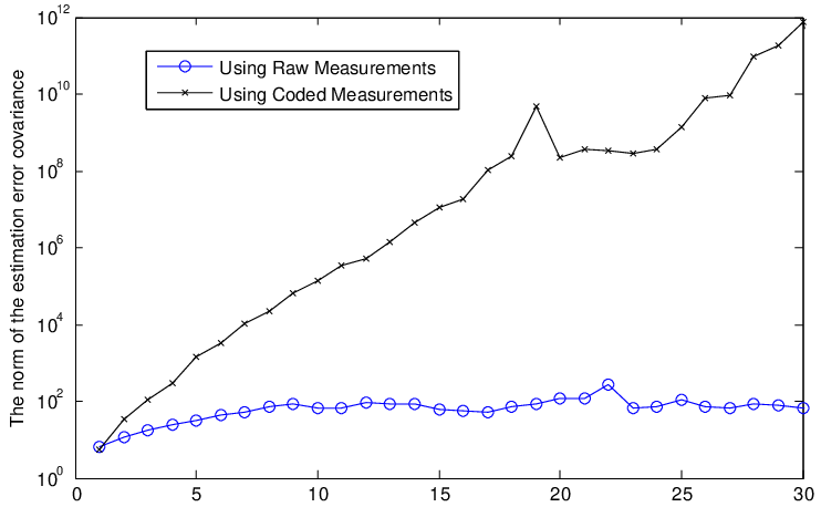
Refer to caption
Figure 3: Norm of prediction error covariance using coded and raw measurements.

7 Conclusion

We studied the networked MMSE state estimation problem for a linear system with a distributed set of sensors. We proposed a measurement coding scheme which permits both, controlling the load of communication used for estimation, and maximizing, within the family of linear causal coders, the robustness of the resulting estimator against packet losses. We derived the resulting MMSE estimator, and state a necessary and sufficient condition, having a trivial gap, for its stability. We quantified the robustness gain offered by the proposed scheme, by comparing the stability condition to the one resulting from the use of raw measurements. We presented simulation results to confirm our claims.

Appendix A Proofs of Lemma 7

Notation 19

Let ℱ​𝒞​ℛ\mathcal{FCR} denote the set of matrices having full column rank.

Let

T¯=[T¯1,⋯,T¯K,T¯∗],\bar{T}=\left[\bar{T}_{1},\cdots,\bar{T}_{K},\bar{T}_{\ast}\right],

be the partition of T¯\bar{T} defined such that, for every kk, the number of columns of T¯k\bar{T}_{k} equals the dimension of JkJ_{k}. We have

D~t,k​Jkt=D¯t​T¯k​Jkt.\tilde{D}_{t,k}J_{k}^{t}=\bar{D}_{t}\bar{T}_{k}J_{k}^{t}. (23)

Now A¯​T¯=T¯​J¯\bar{A}\bar{T}=\bar{T}\bar{J}. Hence, from (8),

A¯​T¯k=T¯​diag​(0,Jk,0)=T¯k​Jk.\bar{A}\bar{T}_{k}=\bar{T}\mathrm{diag}\left(0,J_{k},0\right)=\bar{T}_{k}J_{k}.

Putting the above into (23) we obtain

D~t,k​Jkt=D¯t​A¯t​T¯k.\tilde{D}_{t,k}J_{k}^{t}=\bar{D}_{t}\bar{A}^{t}\bar{T}_{k}. (24)

Now, it is straightforward to see that

A¯t=[At0RtQt],withQ=[00I0],\bar{A}^{t}=\left[\begin{array}[]{cc}A^{t}&0\\ R_{t}&Q^{t}\end{array}\right],\quad\text{with}\quad Q=\left[\begin{array}[]{cc}0&0\\ I&0\end{array}\right], (25)

R0=0R_{0}=0 and, for t>0t>0,

Rt=Rt−1​A+Qt−1​R.R_{t}=R_{t-1}A+Q^{t-1}R. (26)

Putting (25) into (24), and recalling (9), we obtain

D~t,k​Jkt\displaystyle\tilde{D}_{t,k}J_{k}^{t} =Γt​[0Ht]​[At0RtQt]​[TkUk]\displaystyle=\Gamma_{t}\left[\begin{array}[]{cc}0&H_{t}\end{array}\right]\left[\begin{array}[]{cc}A^{t}&0\\ R_{t}&Q^{t}\end{array}\right]\left[\begin{array}[]{c}T_{k}\\ U_{k}\end{array}\right]
=Γt​Ht​[RtQt]​[TkUk]\displaystyle=\Gamma_{t}H_{t}\left[\begin{array}[]{cc}R_{t}&Q^{t}\end{array}\right]\left[\begin{array}[]{c}T_{k}\\ U_{k}\end{array}\right]
=Γt​Ht​Rt​Tk+Γt​Ht​Qt​Uk.\displaystyle=\Gamma_{t}H_{t}R_{t}T_{k}+\Gamma_{t}H_{t}Q^{t}U_{k}.

Now, for t≥Lt\geq L, we have

Rt=[C​At⋮C​At−L+1].R_{t}=\left[\begin{array}[]{c}CA^{t}\\ \vdots\\ CA^{t-L+1}\end{array}\right].

We then obtain

Γt​Ht​Rt​Tk\displaystyle\Gamma_{t}H_{t}R_{t}T_{k}
=\displaystyle= Γt​Ht​[C​At⋮C​At−L+1]​Tk=Γt​Ht​[C​Tk​Jkt⋮C​Tk​Jkt−L+1]\displaystyle\Gamma_{t}H_{t}\left[\begin{array}[]{c}CA^{t}\\ \vdots\\ CA^{t-L+1}\end{array}\right]T_{k}=\Gamma_{t}H_{t}\left[\begin{array}[]{c}CT_{k}J_{k}^{t}\\ \vdots\\ CT_{k}J_{k}^{t-L+1}\end{array}\right]
=\displaystyle= Γt​Ht​[C~k⋮C~k​Jk−L+1]​Jkt=[o~k,t1⋮o~k,tI]\displaystyle\Gamma_{t}H_{t}\left[\begin{array}[]{c}\tilde{C}_{k}\\ \vdots\\ \tilde{C}_{k}J_{k}^{-L+1}\end{array}\right]J_{k}^{t}=\left[\begin{array}[]{c}\tilde{o}_{k,t}^{1}\\ \vdots\\ \tilde{o}_{k,t}^{I}\end{array}\right]
≜\displaystyle\triangleq O~t,k.\displaystyle\tilde{O}_{t,k}.

For t≥Lt\geq L we also have Qt=0Q^{t}=0, and therefore

D~t,k​Jkt\displaystyle\tilde{D}_{t,k}J_{k}^{t} =Γt​Ht​Rt​Tk\displaystyle=\Gamma_{t}H_{t}R_{t}T_{k}
=O~t,k.\displaystyle=\tilde{O}_{t,k}.

We then have that, for t≥Lt\geq L, Ot,T,k∈ℱ​𝒞​ℛ⇔O~t,T,k∈ℱ​𝒞​ℛO_{t,T,k}\in\mathcal{FCR}\Leftrightarrow\tilde{O}_{t,T,k}\in\mathcal{FCR}. Also, for t<Lt<L, we obtain

lim supT→∞ℙ​(Ot,T,k∉ℱ​𝒞​ℛ)1/T\displaystyle~~~~\limsup_{T\rightarrow\infty}\mathbb{P}\left(O_{t,T,k}\notin\mathcal{FCR}\right)^{1/T}
=lim supT→∞ℙ​(Ot,L−t,k∉ℱ​𝒞​ℛ)1/T​ℙ​(OL,T−L,k∉ℱ​𝒞​ℛ)1/T\displaystyle=\limsup_{T\rightarrow\infty}\mathbb{P}\left(O_{t,L-t,k}\notin\mathcal{FCR}\right)^{1/T}\mathbb{P}\left(O_{L,T-L,k}\notin\mathcal{FCR}\right)^{1/T}
=lim supT→∞ℙ​(O~L,T−L,k∉ℱ​𝒞​ℛ)1/T\displaystyle=\limsup_{T\rightarrow\infty}\mathbb{P}\left(\tilde{O}_{L,T-L,k}\notin\mathcal{FCR}\right)^{1/T}
=lim supT→∞ℙ​(O~t,L−t,k∉ℱ​𝒞​ℛ)1/T​ℙ​(O~L,T−L,k∉ℱ​𝒞​ℛ)1/T\displaystyle=\limsup_{T\rightarrow\infty}\mathbb{P}\left(\tilde{O}_{t,L-t,k}\notin\mathcal{FCR}\right)^{1/T}\mathbb{P}\left(\tilde{O}_{L,T-L,k}\notin\mathcal{FCR}\right)^{1/T}
=lim supT→∞ℙ​(O~t,T,k∉ℱ​𝒞​ℛ)1/T,\displaystyle=\limsup_{T\rightarrow\infty}\mathbb{P}\left(\tilde{O}_{t,T,k}\notin\mathcal{FCR}\right)^{1/T},

and the result follows.

Appendix B Proofs of Theorem 10

Let

Et,k=Γt​[Ht1​Gk1⋮HtI​GkI].E_{t,k}=\Gamma_{t}\left[\begin{array}[]{c}H_{t}^{1}G_{k}^{1}\\ \vdots\\ H_{t}^{I}G_{k}^{I}\end{array}\right].

Clearly,

rank⁡(O~t,T,k)=rank⁡([Et,k​Jkt⋮Et+T−1,k​Jkt+T−1]).\mathrm{rank}\left(\tilde{O}_{t,T,k}\right)=\mathrm{rank}\left(\left[\begin{array}[]{c}E_{t,k}J_{k}^{t}\\ \vdots\\ E_{t+T-1,k}J_{k}^{t+T-1}\end{array}\right]\right).

It then follows from Lemma 7 that, for the purposes of computing Φk\Phi_{k}, the pair (Jk,D~t,k)\left(J_{k},\tilde{D}_{t,k}\right) is equivalent to (Jk,Et,k)\left(J_{k},E_{t,k}\right). For S∈𝔻MS\in\mathbb{D}^{M} we use O~t,M,k​(S)\tilde{O}_{t,M,k}(S) to denote the value of O~t,M,k\tilde{O}_{t,M,k} resulting when Γt,M=S\Gamma_{t,M}=S. Let 𝒵t,k⊂𝔻M\mathcal{Z}_{t,k}\subset\mathbb{D}^{M} be the set of all S∈𝔻MS\in\mathbb{D}^{M} such that O~t,M,k​(S)∉ℱ​𝒞​ℛ\tilde{O}_{t,M,k}(S)\notin\mathcal{FCR}.

In order to compute Φk\Phi_{k}, we make use of the result in [15, Proposition 24]. As with [15, Theorem 14], this result is stated under very general assumptions, which are guaranteed by the simpler assumptions given in [15, Proposition 18]. Again, by combining these two results we obtain the following lemma.

Lemma 20.

(Combination of [15, Proposition 18] and [15, Proposition 24]) Consider a FMO block (Jk,Et,k)\left(J_{k},E_{t,k}\right). If Et,kE_{t,k} is a statistically independent sequence of random matrices with discrete distribution and cyclostationary statistics, then

Φk=max0≤t<P⁡maxS∈𝒵t,k​ςt,k​(S)1/M\Phi_{k}=\max_{0\leq t<P}\max_{S\in\mathcal{Z}_{t,k}}\varsigma_{t,k}(S)^{1/M} (29)

where MM is defined in Theorem 5 and

ςt,k(S)=ℙ{ker(O~t,M,k(Γt,M))⊇ker(O~t,M,k(S))}.\varsigma_{t,k}(S)=\mathbb{P}\left\{\ker\left(\tilde{O}_{t,M,k}\left(\Gamma_{t,M}\right)\right)\supseteq\ker\left(\tilde{O}_{t,M,k}\left(S\right)\right)\right\}.

Clearly, the pair (Jk,Et,k)\left(J_{k},E_{t,k}\right) satisfies the conditions in Lemma 20. Hence we can use the result.

We say that node i∈{1,⋯,I}i\in\{1,\cdots,I\} is complete with respect to S∈𝔻MS\in\mathbb{D}^{M} and k∈{1,⋯,K}k\in\left\{1,\cdots,K\right\} if SS includes rk=⌈rank⁡(Ωki)/ci⌉r_{k}=\left\lceil\mathrm{rank}\left(\Omega_{k}^{i}\right)/c_{i}\right\rceil measurements from node ii. Let 𝒞⁡(S)\mathcal{C}(S) denote the set of complete nodes in SS. We have that ker⁡(O~t,M,k​(S~))⊇ker⁡(O~t,M,k​(S))\ker\left(\tilde{O}_{t,M,k}\left(\tilde{S}\right)\right)\supseteq\ker\left(\tilde{O}_{t,M,k}\left(S\right)\right) if S~\tilde{S} misses the same measurements on all nodes not in 𝒞⁡(S)\mathcal{C}(S). We then have

ςt,k​(S)≥∏i∉𝒞⁡(S)(1−pi)M−νi​(S).\varsigma_{t,k}(S)\geq\prod_{i\notin\mathcal{C}(S)}\left(1-p_{i}\right)^{M-\nu^{i}(S)}. (30)

Let 𝒩⁡(S)={0≤νi​(S)≤M:i∉𝒞⁡(S)}\mathcal{N}(S)=\left\{0\leq\nu^{i}(S)\leq M:i\notin\mathcal{C}(S)\right\} . If 𝒞⁡(S)\mathcal{C}(S) is an insufficient set and 𝒩⁡(S)\mathcal{N}(S) are insufficient counts, then S∈𝒵t,kS\in\mathcal{Z}_{t,k}. Combining this with (29) and (30) we obtain

Φk\displaystyle\Phi_{k} ≥max0≤t<P⁡maxℒ​ insufficient​max⁡∏i∉ℒℳ​ insufficient⁡(1−pi)1−MiM\displaystyle\geq\max_{0\leq t<P}\max_{\mathcal{L}\text{ insufficient}}\max_{\mathcal{M}\text{ insufficient}}\prod_{i\notin\mathcal{L}}\left(1-p_{i}\right)^{1-\frac{M^{i}}{M}}
=maxℒ∈𝕃k⁡max⁡∏i∉ℒℳ∈𝕄k​(ℒ)⁡(1−pi)1−MiM.\displaystyle=\max_{\mathcal{L}\in\mathbb{L}_{k}}\max_{\mathcal{M}\in\mathbb{M}_{k}(\mathcal{L})}\prod_{i\notin\mathcal{L}}\left(1-p_{i}\right)^{1-\frac{M^{i}}{M}}. (31)

Suppose that L≥dk,k∈{1,⋯,K}L\geq d_{k},k\in\{1,\cdots,K\} and HtH_{t}, t∈ℕt\in\mathbb{N}, are generated as in Assumption 9. Let S∈𝔻MS\in\mathbb{D}^{M} be such that 𝒞⁡(S)∈𝕃k\mathcal{C}(S)\in\mathbb{L}_{k} and 𝒩⁡(S)∈𝕄k​(𝒞⁡(S))\mathcal{N}(S)\in\mathbb{M}_{k}(\mathcal{C}(S)). Then, w.p.1 over the outcomes of HtH_{t}, any sequence S~\tilde{S} obtained by adding to SS a new measurement from any node i∉𝒞⁡(S)i\notin\mathcal{C}(S) will yield O~t,M,k​(S~)∈ℱ​𝒞​ℛ\tilde{O}_{t,M,k}\left(\tilde{S}\right)\in\mathcal{FCR}. It then follows that ker⁡(O~t,M,k​(S~))⊇ker⁡(O~t,M,k​(S))\ker\left(\tilde{O}_{t,M,k}\left(\tilde{S}\right)\right)\supseteq\ker\left(\tilde{O}_{t,M,k}\left(S\right)\right) if and only if S~\tilde{S} misses the same measurements on all nodes which are incomplete with respect to SS. We then have that (30) and (31) hold with equality, completing the proof.

Appendix C Proofs of Lemma 15

We have

Pk​P|k​P−1\displaystyle P_{kP|kP-1}
≤\displaystyle\leq 𝔼⁡[(xk​P−x^k​P|(k−1)​P−1)​(xk​P−x^k​P|(k−1)​P−1)⊤]\displaystyle\mathbb{E}\left[\left(x_{kP}-\hat{x}_{kP|(k-1)P-1}\right)\left(x_{kP}-\hat{x}_{kP|(k-1)P-1}\right)^{\top}\right]
=\displaystyle= AP​P(k−1)​P|(k−1)​P−1​AP⊤+∑p=0P−1Ap​Q​Ap⊤\displaystyle A^{P}P_{(k-1)P|(k-1)P-1}A^{P\top}+\sum_{p=0}^{P-1}A^{p}QA^{p\top}
≤\displaystyle\leq ρ​(A)2​P​P(k−1)​P|(k−1)​P−1+∑i=0P−1ρ​(A)2​p​Q\displaystyle\rho(A)^{2P}P_{(k-1)P|(k-1)P-1}+\sum_{i=0}^{P-1}\rho(A)^{2p}Q
≤\displaystyle\leq ρ​(A)2​P​P(k−1)​P|(k−1)​P−1+ρ​(A)2​Pρ​(A)2−1​Q,\displaystyle\rho(A)^{2P}P_{(k-1)P|(k-1)P-1}+\frac{\rho(A)^{2P}}{\rho(A)^{2}-1}Q,

and (16) follows since P(k−1)​P|(k−1)​P−1≥QP_{(k-1)P|(k-1)P-1}\geq Q.

Fix kk and put s=(k−1)​P−L+1s=(k-1)P-L+1. For any (k−1)​P≤t<k​P(k-1)P\leq t<kP, it is straightforward to verify that

xt\displaystyle x_{t} =At−s​xs+ϵt−1,s,\displaystyle=A^{t-s}x_{s}+\epsilon_{t-1,s}, (32)
yt\displaystyle y_{t} =C​At−s​xs+εt,s,\displaystyle=CA^{t-s}x_{s}+\varepsilon_{t,s},

where

ϵt−1\displaystyle\epsilon_{t-1} =∑r=1t−sAr−1​wt−r,\displaystyle=\sum_{r=1}^{t-s}A^{r-1}w_{t-r},
εt,s\displaystyle\varepsilon_{t,s} =C​ϵt−1,s+vt.\displaystyle=C\epsilon_{t-1,s}+v_{t}.

Let y¯t⊤=[yt−L+1⊤,⋯,yt⊤]\bar{y}_{t}^{\top}=\left[y_{t-L+1}^{\top},\cdots,y_{t}^{\top}\right] and ε¯t,s⊤=[εt−L+1,s⊤,⋯,εt,s⊤]\bar{\varepsilon}_{t,s}^{\top}=\left[\varepsilon_{t-L+1,s}^{\top},\cdots,\varepsilon_{t,s}^{\top}\right]. We then have

y¯t=F​At−(k−1)​P​xs+ε¯t,s.\bar{y}_{t}=FA^{t-(k-1)P}x_{s}+\bar{\varepsilon}_{t,s}.

Let ut=Γt​ztu_{t}=\Gamma_{t}z_{t}. Then,

ut\displaystyle u_{t} =Γt​Ht​yt¯\displaystyle=\Gamma_{t}H_{t}\bar{y_{t}}
=Γt​Ht​F​At−(k−1)​P​xs+Γt​Ht​ε¯t,s.\displaystyle=\Gamma_{t}H_{t}FA^{t-(k-1)P}x_{s}+\Gamma_{t}H_{t}\bar{\varepsilon}_{t,s}.

Hence, letting Uk⊤=[u(k−1)​P⊤,⋯,uk​P−1⊤]U_{k}^{\top}=\left[u_{(k-1)P}^{\top},\cdots,u_{kP-1}^{\top}\right], we obtain

Uk=Ξk​xs+mt,s,U_{k}=\Xi_{k}x_{s}+m_{t,s}, (33)

where

mt,s\displaystyle m_{t,s} =[Γ(k−1)​P​H(k−1)​P​ε¯(k−1)​P,s⋮Γk​P−1​Hk​P−1​ε¯k​P−1,s].\displaystyle=\left[\begin{array}[]{c}\Gamma_{(k-1)P}H_{(k-1)P}\bar{\varepsilon}_{(k-1)P,s}\\ \vdots\\ \Gamma_{kP-1}H_{kP-1}\bar{\varepsilon}_{kP-1,s}\end{array}\right].

Using (32) and (33), we can obtain an estimate xˇk​P\check{x}_{kP} of xk​Px_{kP} as follows

xˇk​P\displaystyle\check{x}_{kP} =AP​Ξk†​Uk.\displaystyle=A^{P}\Xi_{k}^{\dagger}U_{k}.

If Ξk\Xi_{k} has full column rank, then

xˇk​P\displaystyle\check{x}_{kP} =AP​Ξk†​(Ξk​xs+mt,s)\displaystyle=A^{P}\Xi_{k}^{\dagger}\left(\Xi_{k}x_{s}+m_{t,s}\right)
=AP​xs+Ξk†​mt,s.\displaystyle=A^{P}x_{s}+\Xi_{k}^{\dagger}m_{t,s}.

Then, using (32),

ek\displaystyle e_{k} =xk​P−xˇk​P\displaystyle=x_{kP}-\check{x}_{kP}
=ϵt−1,s−mt,s.\displaystyle=\epsilon_{t-1,s}-m_{t,s}.

Since eke_{k} is only formed by noise terms, it is straightforward to see that there exists a matrix P¯\bar{P} such that, w.p.1 and for all k∈ℕk\in\mathbb{N},

𝔼⁡[ek​ek⊤]≤P¯.\mathbb{E}\left[e_{k}e_{k}^{\top}\right]\leq\bar{P}.

The result then follows after noticing that, since xˇk​P\check{x}_{kP} is a sub-optimal estimator,

Pk​P|k​P−1\displaystyle P_{kP|kP-1} ≤𝔼⁡[ek​ek⊤].\displaystyle\leq\mathbb{E}\left[e_{k}e_{k}^{\top}\right].

Appendix D Proofs of Theorem 17

Let qkiq_{k}^{i}, k∈ℕk\in\mathbb{N}, i∈{1,⋯,I}i\in\{1,\cdots,I\} denote the number of measurements received from sensor ii during the time interval [(k−1)​P,k​P][(k-1)P,kP]. Let 𝒬k={qki:i=1,⋯,I}\mathcal{Q}_{k}=\left\{q_{k}^{i}:i=1,\cdots,I\right\}. For 0≤l≤k0\leq l\leq k, let ℰl,k\mathcal{E}_{l,k} denote the event in which 𝒬l∈ℚ\mathcal{Q}_{l}\in\mathbb{Q} and 𝒬m∉ℚ\mathcal{Q}_{m}\notin\mathbb{Q}, for all m∈{l+1,⋯,k}m\in\{l+1,\cdots,k\}. In particular, notice that ℰ0,k\mathcal{E}_{0,k} denotes the event in which 𝒬m∉ℚ\mathcal{Q}_{m}\notin\mathbb{Q}, for all intervals up to [(k−1)​P,k​P][(k-1)P,kP].

Since HtH_{t}, t∈ℕt\in\mathbb{N}, is pseudo-randomly generated with period P≥nP\geq n, and L≥nL\geq n, it is straightforward to see that, with probability one over the outcomes of HtH_{t}, the matrix QlQ_{l} has full column rank if 𝒬l\mathcal{Q}_{l} is feasible. It then follows from Lemma 15 that

𝔼⁡[Pk​P|k​P−1]\displaystyle\mathbb{E}\left[P_{kP|kP-1}\right] =\displaystyle= ∑l=0k𝔼⁡[Pk​P|k​P−1|ℰl,k]​ℙ​[ℰl,k]\displaystyle\sum_{l=0}^{k}\mathbb{E}\left[P_{kP|kP-1}|\mathcal{E}_{l,k}\right]\mathbb{P}\left[\mathcal{E}_{l,k}\right] (34)
≤\displaystyle\leq ∑l=0kκk−l​𝔼​[Pl​P|l​P−1|ℰl,k]​ℙ​[ℰl,k]\displaystyle\sum_{l=0}^{k}\kappa^{k-l}\mathbb{E}[P_{lP|lP-1}|\mathcal{E}_{l,k}]\mathbb{P}\left[\mathcal{E}_{l,k}\right]
≤\displaystyle\leq ∑l=0kκk−l​ℙ​[ℰl,k]​P¯,\displaystyle\sum_{l=0}^{k}\kappa^{k-l}\mathbb{P}\left[\mathcal{E}_{l,k}\right]\bar{P},

where

κ=ρ​(A)2​P​ρ​(A)2ρ​(A)2−1.\kappa=\rho(A)^{2P}\frac{\rho(A)^{2}}{\rho(A)^{2}-1}.

Let

ϖP=ℙ[𝒬l∉ℚ].\varpi_{P}=\mathbb{P}\left[\mathcal{Q}_{l}\notin\mathbb{Q}\right].

We have

ℙ⁡[ℰl,k]=ϖPk−l​(1−ϖP).\mathbb{P}\left[\mathcal{E}_{l,k}\right]=\varpi_{P}^{k-l}\left(1-\varpi_{P}\right).

By listing all the possibilities of the event 𝒬l∉ℚ\mathcal{Q}_{l}\notin\mathbb{Q}, it follows that

ℙ[𝒬l∉ℚ]=∑𝒬∉ℚ∏i=1I(Pqi)piqi(1−pi)P−qi.\mathbb{P}\left[\mathcal{Q}_{l}\notin\mathbb{Q}\right]=\sum_{\mathcal{Q}\notin\mathbb{Q}}\prod_{i=1}^{I}\binom{P}{q^{i}}p_{i}^{q_{i}}(1-p_{i})^{P-q_{i}}.

Putting the above into (34) yields

𝔼⁡[Pk​P|k​P−1]<(1−ϖP)​P¯​∑l=0k(κ​ϖP)k−l.\mathbb{E}\left[P_{kP|kP-1}\right]<\left(1-\varpi_{P}\right)\bar{P}\sum_{l=0}^{k}\left(\kappa\varpi_{P}\right)^{k-l}.

Hence, supk∈ℕ𝔼⁡[Pk​P|k​P−1]<∞\sup_{k\in\mathbb{N}}\mathbb{E}\left[P_{kP|kP-1}\right]<\infty if

1\displaystyle 1 ≥(κ​ϖP)1/P\displaystyle\geq\left(\kappa\varpi_{P}\right)^{1/P}
=ρ​(A)2​(ρ​(A)2ρ​(A)2−1)1/P​ϖP1/P\displaystyle=\rho(A)^{2}\left(\frac{\rho(A)^{2}}{\rho(A)^{2}-1}\right)^{1/P}\varpi_{P}^{1/P}
=ρ​(A)2​πP1/P,\displaystyle=\rho(A)^{2}\pi_{P}^{1/P},

and (17) the result follows.

Suppose that (A,Ci)(A,C^{i}) is observable for each i=1,…,Ii=1,\ldots,I. Then, 𝒬∉ℚ\mathcal{Q}\notin\mathbb{Q} implies that qi≤nq^{i}\leq n for all i=1,2,…,Ii=1,2,\ldots,I. Thus, we have

limP→∞πP1/P=∏i=1I(1−pi).\lim_{P\rightarrow\infty}\pi_{P}^{1/P}=\prod_{i=1}^{I}(1-p_{i}).

Recall from Section 4.1 that, for each k=1,…,Kk=1,\ldots,K, 𝕃k\mathbb{L}_{k} denotes the collection of all maximal insufficient sets. Since all (A,Ci)(A,C^{i}) are observable, we have 𝕃k=∅\mathbb{L}_{k}=\emptyset. Hence, from Corollary 13, we have

limP→∞Φk=∏i=1I(1−pi)\lim_{P\rightarrow\infty}\Phi_{k}=\prod_{i=1}^{I}(1-p_{i})

for all k=1,…,Kk=1,\ldots,K. Then, (19) follows from the necessary condition stated in Theorem 5.

References

  • [1] V. Gupta, T. Chung, B. Hassibi, and R. Murray. On a stochastic sensor selection algorithm with applications in sensor scheduling and sensor coverage. Automatica, 42(2):251–260, 2006.
  • [2] X. Liu and A. Goldsmith. Kalman filtering with partial observation losses. In Proceedings of 43th IEEE Conference on Decision and Control, pages 4180–4186. IEEE, 2004.
  • [3] B. Sinopoli, L. Schenato, M. Franceschetti, K. Poolla, M. Jordan, and S. Sastry. Kalman filtering with intermittent observations. IEEE Transactions on Automatic Control, 49(9):1453–1464, 2004.
  • [4] L. Schenato, B. Sinopoli, M. Franceschetti, K. Poolla, and S. Sastry. Foundations of control and estimation over lossy networks. Proceedings of the IEEE, 95(1):163–187, 2007.
  • [5] J. Hespanha, P. Naghshtabrizi, and Y. Xu. A survey of recent results in networked control systems. Proceedings of the IEEE, 95(1):138–162, 2007.
  • [6] K. Plarre and F. Bullo. On Kalman filtering for detectable systems with intermittent observations. IEEE Transactions on Automatic Control, 54(2):386–390, 2009.
  • [7] M. Huang and S. Dey. Stability of Kalman filtering with Markovian packet losses. Automatica, 43(4):598–607, 2007.
  • [8] K. You, M. Fu, and L. Xie. Mean square stability for Kalman filtering with markovian packet losses. Automatica, 47(12):2647–2657, 2011.
  • [9] Y. Mo and B. Sinopoli. Towards finding the critical value for Kalman filtering with intermittent observations. http://arxiv.org/abs/1005.2442, 2010.
  • [10] Y. Mo and B. Sinopoli. A characterization of the critical value for kalman filtering with intermittent observations. In 47th IEEE Conference on Decision and Control, pages 2692–2697, 2008.
  • [11] Y. Mo and B. Sinopoli. Kalman filtering with intermittent observations: Tail distribution and critical value. IEEE Transactions on Automatic Control, 57(3):677– 689, 2012.
  • [12] L. Xie and L. Xie. Peak covariance stability of a random Riccati equation arising from Kalman filtering with observation losses. Journal of Systems Science and Complexity, 20(2):262–272, 2007.
  • [13] E. Rohr, D. Marelli, and M. Fu. Kalman filtering for a class of degenerate systems with intermittent observations. In 50th IEEE Conference on Decision and Control and European Control Conference,Orlando, Florida, 2011.
  • [14] E. Rohr, D. Marelli, and M. Fu. Kalman filtering with intermittent observations: On the boundedness of the expected error covariance. IEEE Transactions on Automatic Control, 59(10):2724–2738, 2014.
  • [15] D. Marelli, T. Sui, E. Rohr, and M. Fu. Stability of Kalman Filtering with a random measurement equation: Application to sensor scheduling with intermittent observations. Automatica, 99:390–402, 2019.
  • [16] K. Okano and H. Ishii. Stabilization of uncertain systems using quantized and lossy observations and uncertain control inputs. Automatica, 81:261–269, 2017.
  • [17] F. Smarra, M. Benedetto, and A. Innocenzo. Efficient routing redundancy design over lossy networks. International Journal of Robust and Nonlinear Control, 28(6):2574–2597, 2018.
  • [18] L. Schenato. Optimal estimation in networked control systems subject to random delay and packet drop. IEEE Transactions on Automatic Control, 53(5):1311–1317, 2008.
  • [19] R. Koetter and M. Medard. An algebraic approach to network coding. IEEE/ACM Transactions on Networking, 11(5):782–795, 2003.
  • [20] E. Erez, M. Kim, Y. Xu, Yeh. E, and M. Medard. Deterministic network model revisited: An algebraic network coding approach. IEEE Transactions on Information Theory, 60(8):4867–4879, 2014.
  • [21] L. He, D. Han, X. Wang, and L. Shi. Optimal linear state estimation over a packet-dropping network using linear temporal coding. Automatica, 49(4):1075–1082, 2013.
  • [22] T. Sui, K. You, M. Fu, and D. Marelli. Stability of MMSE state estimators over lossy networks using linear coding. Automatica, 51(1):167–174, 2015.
  • [23] X. He, Z. Wang, X. Wang, and D. Zhou. Networked strong tracking filtering with multiple packet dropouts: algorithms and applications. IEEE Transactions on Industrial Electronics, 61(3):1454–1463, 2014.
  • [24] J. Hu, Z. Wang, and H. Gao. Recursive filtering with random parameter matrices, multiple fading measurements and correlated noises. Automatica, 49(11):3440–3448, 2013.
  • [25] J. Hu, Z. Wang, H. Gao, and L. Stergioulas. Extended kalman filtering with stochastic nonlinearities and multiple missing measurements. Automatica, 48(9):2007–2015, 2012.
  • [26] G. Wei, Z. Wang, and H. Shu. Robust filtering with stochastic nonlinearities and multiple missing measurements. Automatica, 45(3):836–841, 2009.
  • [27] S. Deshmukh, B. Natarajan, and A. Pahwa. State estimation over a lossy network in spatially distributed cyber-physical systems. IEEE Transactions on Signal Processing, 62(15):3911–3923, 2014.
  • [28] D. Quevedo, A. Ahlén, and K. Johansson. State estimation over sensor networks with correlated wireless fading channels. IEEE Transactions on Automatic Control, 58(3):581–593, 2013.
  • [29] K. Gatsis, M. Pajic, A. Ribeiro, and G. Pappas. Opportunistic control over shared wireless channels. IEEE Transactions on Automatic Control, 60(12):3140–3155, 2015.
  • [30] T. Sui, K. You, and M. Fu. Stability conditions for multi-sensor state estimation over a lossy network. Automatica, 53(3):1–9, 2015.
  • [31] B. Anderson and B. Moore. Optimal Filtering. Prentice-hall & Systems Sciences Series, New Jersey, 1979.