Phase Diagram and Quench Dynamics in a Spinful Interacting Kitaev Chain

In the last decades topological materials have received a great attention. Although a systematic study can be performed for non-interacting fermions schnyder08; kitaev08; chiu16, the role of interactions remains particularly attractive because it leads to a breakdown of this classification Fidowski10.

Unfortunately, interacting models which can be exactly solvable are uncommon. For example, one dimensional models like the Hubbard and Heisenberg models and some of their generalizations can be solved through a Bethe ansatz technique takashi; korepin; kawakami.

The Kitaev chain model in the presence of nearest neighbor interaction has been recently characterized by considering a frustration-free case katsura15 with a non-homogenous chemical potential Wouters18, and an exact solution has been given at the symmetric point Miao17 by also including dimerization Ezawa17; Wang17. Another exactly solvable model which is a p-wave chain of spin $\frac{1}{2}$ fermions in presence of Hubbard interaction has been introduced by Mattis and Nam Mattis72. That model can be mapped onto two interacting Kitaev chains, which have been recently taken in exam outside the half-filling by adopting numerical methods and bosonization technics Herviou16.

A common aspect of these models is the presence of a topological non trivial ground state and the potential to describe a topological transition due to the interaction. In this context, the study of out of equilibrium dynamics of many-body systems following a quench, i.e an abrupt change of some control parameter of the system, can contain rich effects as it is typically related to the topological features of the achieved quantum phases. In particular, in one dimensional topological systems of non-interacting fermions, quench between distinct topologically phases are intimately related to the emergence of dynamical phase transitions heyl18. Moreover, the dynamics following a local quench allows to study the propagation of quasiparticles in the system, which has been already analysed in a one dimensional quantum Ising chain smacchia12; francica16.

In this paper, starting from the Mattis-Nam model we consider the role of interacting terms that favor the generation of effective molecular-like configurations in the ground state. An exact solution in terms of non-interacting spinless fermions can be achieved by performing two Jordan-Wigner transformations. We provide a characterization of the quantum phase in the bulk and at the boundary of the chain, highlighting the presence of long range order in the trivial phases related to a spontaneous symmetry breaking of the $Z_{2}^{x}$ symmetry corresponding to a rotation by $\pi$ with respect to the $x$ axis in the spin space. We demonstrate that the model is exactly solvable also in the presence of boundary interactions originating from a spin-singlet superconducting pairing and a magnetic field along a specific direction. We also analyse the dynamics in the Mattis-Nam model due to a boundary quench by examining the propagation of disturbance in the nearest-neighbor magnetization and spin-singlet correlations. Both display a ballistic long time propagation with sensitively different velocities.

The paper is structured in the following way. In the Sect. II we introduce the model summarizing its main symmetries. The Sect. III is devoted to the exact solution of the model. In Sec. IV we characterize the quantum phases from a topological point of view and in terms of the ground-state correlations. We also give a dynamically characterization by performing a quench at the boundary of the chain. Sec. V is devoted to the summary of the results achieved and conclusions.

We consider a one-dimensional chain of spin $\frac{1}{2}$ fermions described by the Hamiltonian $H=H_{0}+H_{1}+H_{edge}$.

For a chain of length $L$ with open boundary conditions, the Hamiltonian $H_{0}$ reads

The term $H_{1}$ reads

We take into account boundary interactions described by $H_{edge}$, originating from the presence of a singlet superconductive pairing $\Delta_{0}$ and a magnetic field $\mathbf{h}=(h_{x},h_{y},h_{z})$

We assume an equal spin pairing triplet pairing, such that the order parameter has the same amplitude in both spin up and down channels $\Delta_{\uparrow}=\Delta_{\downarrow}=\Delta$.

Moroever, one can exploit the transformation $(c_{j\uparrow},c_{j\downarrow})\to(c_{j\uparrow},ic_{j\downarrow})$ to explore the case of a spin triplet superconductor having opposite sign between the spin up and down triplet pairing. In terms of the $d$-vector representation, it implies that one can both investigate the case with $d_{x}$ and $d_{y}$ spin triplet pairing. The interaction transforms as $H_{1}\mapsto\sum_{j}\lambda_{j}(2n_{2j\uparrow}-1)(2n_{2j-1\downarrow}-1)$, i.e. a dimerized nearest-neighbor Hubbard interaction, and the boundary couplings as $\mathbf{h}\mapsto(h_{y},h_{x},h_{z})$ and $\Delta_{0}\mapsto i\Delta_{0}$.

We briefly recall the symmetry features of the model without the boundary term $H_{edge}$.

The model is symmetric with respect to the time-reversal transformation which is represented by an anti-unitary operator which acts on the fermions as $(c_{j\uparrow},c_{j\downarrow})\to(c_{j\downarrow},-c_{j\uparrow})$ and with respect to the number parity transformation represented by the unitary operator $Z^{f}_{2}=e^{i\pi\sum n_{j\sigma}}$. The model is invariant also under the rotation $(c_{j\uparrow},c_{j\downarrow})\to(c_{j\downarrow},c_{j\uparrow})$ represented through the unitary operator $Z^{x}_{2}$.

At $\Delta=0$ there is a spin rotation symmetry $SU(2)$, which is broken down to the rotation around $y$ axis

At $\mu=0$ the model is invariant under the particle-hole transformation $c_{i\sigma}\to(-1)^{i}c^{\dagger}_{i\sigma}$, so that $Z^{p}_{2}=\prod_{j\sigma}(c_{j\sigma}+(-1)^{j}c^{\dagger}_{j\sigma})$ is conserved. We note that all the operators $Z^{\gamma}_{2}$ (with $\gamma=f,p,x$) squares to the identity (we consider $L$ even).

Conversely, both the boundary interaction terms always break the time-reversal and the rotation $Z^{x}_{2}$ symmetries.

Because of the presence of the quartic terms, the Hamiltonian $H$ cannot be diagonalized in straightforward way.

In this paper we consider the symmetric point $\Delta=t$ at half-filling $\mu=0$, a magnetic field $\mathbf{h}=h\hat{\mathbf{y}}$ and $\lambda_{j}=\lambda$ homogenous.

We rewrite the Hamiltonian in the Majorana fermion representation by defining the real Majorana operators $a_{j\sigma}=c_{j\sigma}+c^{\dagger}_{j\sigma}$ and $b_{j\sigma}=-ic_{j\sigma}+ic^{\dagger}_{j\sigma}$ which satisfy relations $\{a_{i\sigma},a_{j\sigma^{\prime}}\}=\{b_{i\sigma},b_{j\sigma^{\prime}}\}=2\delta_{ij}\delta_{\sigma\sigma^{\prime}}$ and $\{a_{i\sigma},b_{j\sigma^{\prime}}\}=0$.

In this representation the Hamiltonian $H_{0}$ reads

By performing two Jordan-Wigner transformations, we map the Hamiltonian $H$ onto the simpler fermionic model ¹¹ 1 See appendix for details.

The parities map onto $Z_{2}^{f}=\prod_{j}^{L}(ia_{j}b_{j})$ and $Z_{2}^{p}=\prod_{j}^{L}(ic_{j}d_{j})$.

All the eigenstates of the interacting model can be classified in terms of the eigenvalues $r_{j}$ of the operators $R_{j}$, and the model can be exactly solvable in each of these subspaces. In details for the configuration $\{r_{j}\}$ we obtain a quadratic fermionic Hamiltonian $H=\frac{i}{2}\sum a_{i}B_{ij}b_{j}+c_{0}r_{L}+\lambda\sum_{i=1}^{\frac{L}{2}}r_{2i}r_{2i-1}$ with $\mathbf{B}$ a real matrix with non zero elements $B_{i,i+1}=-2(r_{i}+r_{i+1})t$, $B_{ii}=-2U$ for $i<L$ and $B_{LL}=-2\alpha U$ with $\alpha$ defined such that $\alpha U=\frac{1}{2}(\Delta_{0}+h/2)r_{L}+U$. By performing the singular value decomposition $\mathbf{B}=\mathbf{U}\boldsymbol{\Lambda}\mathbf{V}^{T}$ with $\mathbf{U}$ and $\mathbf{V}$ real orthogonal matrices and $\boldsymbol{\Lambda}$ semi-definite positive diagonal matrix with diagonal elements $\Lambda_{k}\geq 0$, the Hamiltonian can be written in the canonical form $H=\frac{i}{2}\sum_{k}\Lambda_{k}\tilde{a}_{k}\tilde{b}_{k}$ where $\tilde{a}_{k}=\sum_{i}U_{ik}a_{i}$ and $\tilde{b}_{k}=\sum_{i}V_{ik}b_{i}$ and depend on the configuration $\{r_{j}\}$. The minimum energy in that sector results to be $E=-\sum_{k}\Lambda_{k}/2+c_{0}r_{L}+\lambda\sum_{i}r_{2i}r_{2i-1}$. By focusing on the model without the boundary term $H_{edge}$, the two configurations $\{r_{j}\}$ and $\{-r_{j}\}$ give same energy spectrum due to the $Z^{x}_{2}$ symmetry.

The Mattis-Nam Hamiltonian $H_{0}$ has been previously characterized in ref. Mattis72, and in the following we clarify how the term $H_{1}$ changes the phase of the model.

A non-homogenous $r_{j}$ produces disjoint molecules (i.e. Kitaev chains) in Eq. (5) and for an attractive interaction $H_{1}$ ($\lambda<0$) the ground state energy is obtained for the two homogenous cases $\{r_{i}=1\}$ and $\{r_{i}=-1\}$ due to the lowering in energy coming from the molecules union.

Conversely, for $\lambda>0$ there is a lowering in energy as the configuration $\{r_{i}\}$ becomes non-homogeneous due to the $H_{1}$ term which gets its minimum value $-\lambda L/2$ for the two staggered cases $\{r_{2j-1}=(-1)^{j+1},r_{2j}=(-1)^{j}\}$ and $\{r_{2j-1}=(-1)^{j},r_{2j}=(-1)^{j+1}\}$.

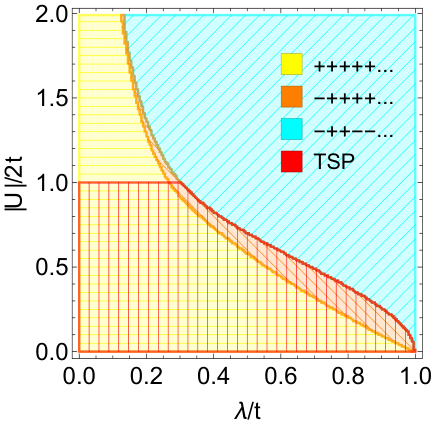
For $U=0$, the ground state energy is obtained for the homogenous configurations if $\lambda<t$ and for the staggered ones if $\lambda>t$. For $U\neq 0$ a numerical analysis shows that the ground state energy is obtained also for $r_{j}$ homogenous everywhere except the edges, i.e. homogenous only for $1<j<L$ (see Fig. 1).

Then in the bulk we have two distinct ground state sectors corresponding to the staggered (cyan region in Fig. 1) and homogenous configurations (yellow and orange regions in Fig. 1) due to the presence of the interaction $H_{1}$.

In the two sectors $\{r_{i}=1\}$ and $\{r_{i}=-1\}$ the model with boundary interactions reads

For $c_{0}=0$, for every value of $U$ there are two ground states $\left|0_{\pm}\right\rangle$ belonging to the two subspaces $\{r_{j}=\pm 1\}$ defined as the vacuum states such that $i\tilde{a}_{k\pm}\tilde{b}_{k\pm}\left|0_{\pm}\right\rangle=-\left|0_{\pm}\right\rangle$ for every $k$ and characterized by an even fermionic parity $\left\langle 0_{\pm}\right|Z^{f}_{2}\left|0_{\pm}\right\rangle=1$. We observe that the two states are related via the transformation $Z^{x}_{2}$. This degeneration will be lifted due the presence of the term $H_{edge}$ for $c_{0}\neq 0$, and their energy will be $E_{\pm}=-\frac{1}{2}\sum_{k}\Lambda_{k}\pm c_{0}+\lambda L/2$.

We note that the symmetry $Z^{p}_{2}$ can be expressed as the product of the two operators $Z^{p}_{2}=\prod_{\sigma}Z^{p}_{2,\sigma}$ which shows the critical behavior

The degeneration at $c_{0}=0$ is due to the presence of the symmetry under the composition $Z^{x}_{2}T$, where $T$ is the time reversal transformation.

Without the edge term $H_{edge}$, we recall that in absence of interactions ($U=0$ and $\lambda=0$) the quantum phase exhibits a doublet of Majorana fermions at each edge. Then, in the presence of interactions we have a topological phase in the adiabatically connected red region, i.e. until we reach the phase transition line $U=\pm 2t$ and $\lambda<\lambda_{c}$ at which the model is gapless, or until we reach a level crossing and the configuration $r_{j}$ becomes staggered.

We argue that the topological phase belongs to the class of topologically symmetry protected (TSP) states Fidowski11. We recall that the model is characterized through a time reversal symmetry represented by the antiunitary operator $T$, such that $T^{2}=-1$, and the fermionic parity $Z^{f}_{2}$, commutating each other. At the left boundary of the chain for $U=\lambda=0$ we consider the Hilbert space of the Majorana fermions $a_{1\uparrow}$, $a_{1\downarrow}$. By defining the complex fermion $c=\frac{1}{2}(a_{1\uparrow}+ia_{1\downarrow})$, the transformations $Z^{f}_{2}$ and $T$ are locally represented through $\hat{Z}^{f}_{2}=(-1)^{c^{\dagger}c}$ and $\hat{T}=(c-ic^{\dagger})K$ ($K$ being the complex conjugate operator), which implies that $\hat{T}^{4}=-1$ and $\hat{Z}^{f}_{2}\hat{T}=-\hat{T}\hat{Z}^{f}_{2}$ until the ground state remains gapped.

Instead, in the two sectors $\{r_{2j-1}=(-1)^{j+1},r_{2j}=(-1)^{j}\}$ and $\{r_{2j-1}=(-1)^{j},r_{2j}=(-1)^{j+1}\}$ we have a sum of disjoint molecules

In the following we briefly summarize the main features of the quantum phases, by considering the thermodynamic limit $L\to\infty$.

We start by considering the homogenous cases $\{r_{j}=1\}$ and $\{r_{j}=-1\}$, i.e. the Hamiltonian $H_{0}$ is dominant over $H_{1}$.

Local spin-singlet correlations tend to be formed for an attractive interaction and antiferromagnetic order for a repulsive one. For $\alpha=1$ the ground state shows spin-singlet correlations at the boundary, which are given by

The boundary magnetization in the $y$ direction is related to the singlet correlation through the equation $\langle S^{y}_{L}\rangle=-i\langle c_{L\uparrow}c_{L\downarrow}\rangle-\frac{r_{L}}{2}$, so that $\langle S^{y}_{L}\rangle\approx 0$ for $U\ll-2t$ and $\langle S^{y}_{L}\rangle\approx\frac{r_{L}}{2}$ for $U\gg 2t$. When the boundary interactions are such that $\alpha=0$, in the correspondent subspace the real fermion $a_{L}$ is decoupled, and at finite size the boundary spin-singlet correlator tends to be

On the other side, when $H_{1}$ is dominant and the configuration $\{r_{2j}=(-1)^{j},r_{2j-1}=(-1)^{j+1}\}$ are selected, the phase is characterized by the correlations

For this model we note that the exact solution allows us to explore which role a non-homogenous interaction $\underline{U}=(U_{1},U_{2},\cdots,U_{L})$ plays, where $U_{i}$ is its value on the site $i$. As an example, we consider $\lambda=0$ and a pattern $\underline{U}=(x,\cdots,x,1,x,\cdots,x,1,x\cdots)U$ where the value $U$ is repeated in steps of $N$. From a numeric calculation of the Majorana number for the model in Eq. (6) it results that the phase is expected to be topologically nontrivial if $t>\beta_{N}(x)\left|U\right|$ where the linear coefficient $\beta_{N}(x)$ decreases to zero as $x\to 0$ and to $x/2$ as $N\to L$. The same result is observed by considering random distributions of the interaction $U$ in the pattern $\underline{U}$, with a linear coefficient that decreases with the occurrence of the values $x$ in $\vec{U}$. This analysis proves how the topological phase is strong against a sparse interaction ($x=0$) in the chain.

We now proceed giving a characterization of the dynamics features. By changing in time $\tau$ the on-site interaction $U$, we produce the power $\mathcal{P}=\langle\dot{H}(\tau)\rangle=\dot{U}\sum_{j=1}^{L}\langle-ia_{j}(\tau)b_{j}(\tau)\rangle$. A particularly interesting case arises when considering the driving across the critical line $U=\pm 2t$ and $\lambda<\lambda_{c}$ which gives a nonzero power due to the production of adiabatic excitations related to the second order quantum phase transition. As an example, we consider a turn-on of a strong interaction $U\gg 2t$ which is linear in time with speed $\dot{U}=1/\tau_{Q}$. Due to the relation to the Ising model, we have the power density $\frac{\mathcal{P}}{L}\sim\frac{1}{2\pi}\frac{\dot{U}}{2t\sqrt{2\tau_{Q}}}$ Dziarmaga05.

We now turn to the study of the dynamics in the non-insulating phase following the sudden turn-off of the boundary interactions. With the aim to show how a local perturbation propagates in the interacting chain, we assume the system to be initially prepared in the ground state of $H$ (with $\alpha=0^{+}$). At $\tau=0$ the boundary interaction is suddenly switched-off ($\alpha=1$ for $\tau>0$), so that the time evolution is generated by the Mattis-Nam Hamiltonian $H_{0}$. The dynamics remains in the invariant subspace with homogenous $r_{j}$, giving a ballistic propagation of the signal.

In particular, the density of particles is constant $\langle n_{j\sigma}\rangle=\frac{1}{2}$, so that the propagation occurs with a zero normal current.

We consider how the nearest neighbor charge and spin correlations $C_{i}(\tau)=\langle c_{i\uparrow}(\tau)c_{i\downarrow}(\tau)c^{\dagger}_{i+1\downarrow}(\tau)c_{i+1\uparrow}^{\dagger}(\tau)\rangle$ and $S_{i}(\tau)=\langle S^{y}_{i}(\tau)S^{y}_{i+1}(\tau)\rangle$ evolve in time after a local sudden quench generated by changing the edge term at the initial time $\tau=0$. By considering the mean square center $R_{f}^{2}(\tau)=(1/L)\sum_{i}f_{i}(\tau)(i-L)^{2}$ where $f=C,S$, we numerically find that the velocity $v_{f}(\tau)=\partial_{\tau}\sqrt{\left|R_{f}^{2}(\tau)-R_{f}^{2}(0)\right|}$ tends to be constant for $\tau\gg 1$ (see fig. 2), so that the propagation is ballistic.

We note that the difference in the propagation velocities $v_{C}$ and $v_{S}$ is due to how the modes interfere, producing a spin-charge separation effect.

In conclusion we have characterized the static and dynamical properties of the Mattis-Nam model in the presence of both nearest-neighbor interactions and magnetic and superconducting couplings at the boundary. The model is shown to be exactly solvable by a mapping onto a non-interacting one, allowing to give a direct access to the characterization of the quantum phase diagram. Due to the new interaction an insulating phase emerges with an electronic pattern which is marked by effective disjoint molecular-like configurations. The mean features of the different phases have been characterized from a topological point of view, and by looking at the superconducting spin-singlet and magnetic correlations. In particular the topological phase exhibits four Majorana fermions in absence of quartic interactions, and by turning-on these interactions the model can undergo a transition into trivial phases. Remarkably, we find that the transition into the insulating region occurs via a distinct inhomogeneous intermediate phase showing edges disjoint from the bulk. We provide a characterization also from a dynamical point of view by considering the evolution due to a quench generated by suddenly removing the boundary term. The outcome highlights the possibility of obtaining a propagation as a function of the Hubbard interaction strength for the magnetic and superconducting correlators with significantly different velocities.

References

• (1) A. P. Schnyder, S. Ryu, A. Furusaki, and A. W. W. Ludwig, Phys. Rev. B 78, 195125 (2008).
• (2) A. Yu. Kitaev, arXiv:0901.2686 .
• (3) C.-K. Chiu, J. C. Y. Teo, A. P. Schnyder, and S. Ryu, Rev. Mod. Phys. 88, 035005 (2016).
• (4) L. Fidkowski and A. Kitaev, Phys. Rev. B 81, 134509 (2010).
• (5) L. Fidkowski and A. Kitaev, Phys. Rev. B 83, 075103 (2011).
• (6) L. Herviou, C. Mora, and K. Le Hur, Phys. Rev. B 93, 165142 (2016).
• (7) M. Takahashi, Thermodynamics of One-Dimensional Solvable Models, Cambridge University Press (2019). (DOI: https://doi.org/10.1017/CBO9780511524332)
• (8) V. E. Korepin and F. L. Essler, Exactly Solvable Models of Strongly Correlated Electrons, World Scientific (1994). (DOI:https://doi.org/10.1142/2148).
• (9) N. Kawakami and A. Okiji, Progress of Theoretical Physics Supplement 108, 251 (1992) (DOI: 10.1143/PTPS.108.251)
• (10) H. Katsura, D. Schuricht, and M. Takahashi, Phys. Rev. B 92, 115137 (2015).
• (11) J. Wouters, H. Katsura, D. Schuricht, Phys. Rev. B 98, 155119 (2018).
• (12) J.-J. Miao, H.-K. Jin, F.-C. Zhang, and Y. Zhou, Phys. Rev. Lett. 118 267701 (2017).
• (13) M- Ezawa, Phys. Rev. B 96, 121105(R) (2017).
• (14) Y. Wang, J.-J. Miao, H.-K. Jin, and S. Chen Phys. Rev. B 96, 205428 (2017).
• (15) W. Brzezicki and A. Oleś, Phys. Rev. B 80, 014405 (2009).
• (16) W. DeGottardi, D. Sen and S. Vishveshwara, New Journal of Physics 13, 065028 (2011).
• (17) D. C. Mattis and S. B. Nam, Journal of Mathematical Physics 13, 1185 (1972).
• (18) J. Dziarmaga, Phys. Rev. Lett. 95, 245701 (2005).
• (19) G. Francica, T. J. G. Apollaro, N. Lo Gullo, and F. Plastina, Phys. Rev. B 94, 245103 (2016).
• (20) P. Smacchia and A. Silva, Phys. Rev. Lett. 109, 037202 (2012).
• (21) M. Heyl, Rep. Prog. Phys. 81 054001 (2018).