Dispersion and reaction in random flows:
single realisation vs ensemble averagePreprint: APS/123-QED

We restrict our attention to flows $\bm{u}$ that are random in time, with stationary statistics, zero mean, and finite correlation time, and $2\pi$-periodic in space with vanishing spatial average. We show that flows in this class satisfy $\mathrm{K}=\overline{\rm K}$, hence that the single-realisation and ensemble-averaged scalar fields $C$ and $\mathbin{\left\langle C\right\rangle}$ are equivalent in the diffusive approximation. We start by averaging (2) with respect to both the Brownian motion and the velocity realisation. This gives $\mathbin{\langle\mathbb{E}\left[\bm{\bm{X}\left(t\right)}\right]\rangle}=\bm{0}$, since $\mathbin{\langle\bm{u}(\cdot,t)\rangle}=0$, hence

and

using (10). We now show that $\left\|\mathbin{\langle\mathbb{E}\left[\bm{X}\left(t\right)\right]\otimes\mathbb{E}\left[\bm{X}\left(t\right)\right]\rangle}\right\|=o\left(t\right)$.

In order to estimate $\mathbb{E}\left[\bm{X}\left(t\right)\right]$, we introduce the expected displacement at time $t$ of a particle initially located at $\bm{x}$,

such that $\mathbb{E}\left[\bm{X}\left(t\right)\right]={\mathchoice{\raisebox{0.0pt}{$\displaystyle\bm{\chi}$}}{\raisebox{0.0pt}{$\textstyle\bm{\chi}$}}{\raisebox{0.0pt}{$\scriptstyle\bm{\chi}$}}{\raisebox{0.0pt}{$\scriptscriptstyle\bm{\chi}$}}}\left(0,t\right)$. The expectation in (13) satisfies the backward Kolmogorov equation (e.g. Øksendal 1998, Ch. 8)

hence $\textstyle\bm{\chi}$ satisfies the corresponding forced equation

with the initial condition ${\mathchoice{\raisebox{0.0pt}{$\displaystyle\bm{\chi}$}}{\raisebox{0.0pt}{$\textstyle\bm{\chi}$}}{\raisebox{0.0pt}{$\scriptstyle\bm{\chi}$}}{\raisebox{0.0pt}{$\scriptscriptstyle\bm{\chi}$}}}\left(\bm{x},0\right)=\bm{0}$. Since $\bm{u}$ and the initial condition ${\mathchoice{\raisebox{0.0pt}{$\displaystyle\bm{\chi}$}}{\raisebox{0.0pt}{$\textstyle\bm{\chi}$}}{\raisebox{0.0pt}{$\scriptstyle\bm{\chi}$}}{\raisebox{0.0pt}{$\scriptscriptstyle\bm{\chi}$}}}\left(\bm{x},0\right)$ are both spatially periodic, the solution $\textstyle\bm{\chi}$ of Eq. (15) is spatially periodic. The cell-integrated variance

where $\mathcal{A}$ denotes spatial averaging over a periodic cell, is found from (15) to satisfy

using integration by parts and the incompressibility condition $\nabla\cdot\bm{u}=0$ and where $\|\|.\|\|$ denotes the Frobenius norm. We bound the right-hand side of (17) in terms of $\sigma$. Averaging Eq. (15) and using that $\mathcal{A}\left[\bm{u}\right]=0$ gives $\mathcal{A}\left[{\mathchoice{\raisebox{0.0pt}{$\displaystyle\bm{\chi}$}}{\raisebox{0.0pt}{$\textstyle\bm{\chi}$}}{\raisebox{0.0pt}{$\scriptstyle\bm{\chi}$}}{\raisebox{0.0pt}{$\scriptscriptstyle\bm{\chi}$}}}\right]=0$. This enables us to use the Poincaré inequality for the term $\mathcal{A}\left[\|\|\nabla{\mathchoice{\raisebox{0.0pt}{$\displaystyle\bm{\chi}$}}{\raisebox{0.0pt}{$\textstyle\bm{\chi}$}}{\raisebox{0.0pt}{$\scriptstyle\bm{\chi}$}}{\raisebox{0.0pt}{$\scriptscriptstyle\bm{\chi}$}}}\|\|^{2}\right]$ and the Cauchy–Schwarz inequality for the term $\mathcal{A}\left[\bm{u}\cdot{\mathchoice{\raisebox{0.0pt}{$\displaystyle\bm{\chi}$}}{\raisebox{0.0pt}{$\textstyle\bm{\chi}$}}{\raisebox{0.0pt}{$\scriptstyle\bm{\chi}$}}{\raisebox{0.0pt}{$\scriptscriptstyle\bm{\chi}$}}}\right]$. This yields the differential inequality

where the domain is taken as $[0,2\pi]^{d}$ so that the Poincaré constant is $1$ and $U=\mathbin{\langle\mathcal{A}[|{\bm{u}}|^{2}]\rangle}^{1/2}$ is the root-mean-square velocity. Integrating in time, we obtain

The Laplacian operator in Eq. (15) ensures that the solution $\textstyle\bm{\chi}$ is smooth, so the boundedness of $\sigma$ guaranteed by (19) implies that $\mathbin{\left\langle|{\mathchoice{\raisebox{0.0pt}{$\displaystyle\bm{\chi}$}}{\raisebox{0.0pt}{$\textstyle\bm{\chi}$}}{\raisebox{0.0pt}{$\scriptstyle\bm{\chi}$}}{\raisebox{0.0pt}{$\scriptscriptstyle\bm{\chi}$}}}|^{2}\left(0,t\right)\right\rangle}$ is also bounded. Finally, observing that $\left\|\mathbin{\langle\mathbb{E}\left[\bm{X}\left(t\right)\right]\otimes\mathbb{E}\left[\bm{X}\left(t\right)\right]\rangle}\right\|=O\left(\mathbin{\left\langle|{\mathchoice{\raisebox{0.0pt}{$\displaystyle\bm{\chi}$}}{\raisebox{0.0pt}{$\textstyle\bm{\chi}$}}{\raisebox{0.0pt}{$\scriptstyle\bm{\chi}$}}{\raisebox{0.0pt}{$\scriptscriptstyle\bm{\chi}$}}}|^{2}\left(0,t\right)\right\rangle}\right)=O(1)=o\left(t\right)$ we conclude that $\mathrm{K}=\overline{\mathrm{K}}$.

We note that the upper bound $U^{2}/\kappa^{2}$ found in (19) is far from optimal. We also note that the argument above relies crucially on the assumption $\mathcal{A}\left[\bm{u}\right]={\bf 0}$. Without this premise, it is possible that $\mathrm{K}\neq\overline{\mathrm{K}}$. As an example, consider the case of a spatially uniform 2D flow with constant magnitude $U$ whose direction changes randomly every unit time. Such a flow has a non-zero spatial average but its ensemble average vanishes. Computing the two diffusivity tensors is straightforward and gives $\mathrm{K}=\kappa\mathbb{I}_{d}$ and $\overline{\mathrm{K}}=\left(\kappa+U/4\right)\mathbb{I}_{d}$, where $\mathbb{I}_{d}$ is the $d\times d$ identity matrix.

In this subsection, we compare the diffusive approximation of $C_{n}$ and $\mathbin{\left\langle C_{n}\right\rangle}$ for the alternating sine model introduced in section II. We introduce the finite-time velocities

and the finite-time diffusivity tensors

which converge to $\bm{v}$, $\overline{\bm{v}}$, $\mathrm{K}$ and $\overline{\rm K}$ in the large-$n$ limit.

The discrete-time equivalent of (2) associated with the map (6) is the random walk for the position $\bm{X}_{n}=\left(X_{n},Y_{n}\right)$ of a single scalar particle,

where the $\bm{W}_{n}$ are independent Gaussian variables with zero mean and unit variance. Starting from $\bm{X}_{0}=\bm{0}$, the scalar field $C_{n}$ satisfying (6), once suitably normalised, is the probability density function

of the particle position, with $\mathbb{E}$ denoting the expectation with respect to the Gaussian variables $\bm{W}_{n}$ associated to the molecular diffusion. Taking ${\bm{X}}_{0}={\bm{0}}$ corresponds to a Dirac initial condition $C_{0}\left(\bm{x}\right)=\delta\left(\bm{x}\right)$, which we employ in what follows.

For the alternating sine flow, each realisation is defined by a sequence of phases $(\varphi_{n},\psi_{n})$, so the ensemble average is

where $\bm{\varphi}=\left(\varphi_{0},\dots,\varphi_{n-1}\right)$ and $\bm{\psi}=\left(\psi_{0},\dots,\psi_{n-1}\right)$. We note that

which is readily established by the substitution $\phi_{n}\mapsto\phi_{n}-y$ in the integral (24) defining the ensemble average. Similarly,

As a result, $\mathbin{\left\langle C_{n}\right\rangle}$ can be obtained as the ensemble-averaged probability density function

associated with the modified random walk

This has the advantage over (22) that the position after $n$ steps can be written explicitly as

where $\bm{W}$ is a single Gaussian variable with zero mean and unit variance.

Replacing ${\bm{X}}_{n}$ by $\tilde{\bm{X}}_{n}$ leaves the ensemble-averaged statistics unchanged, as Eq. (27) shows, while making their computation straightforward. We can in particular compute $\overline{\bm{v}}_{n}$ and $\overline{\rm K}_{n}$ by substituting $\tilde{\bm{X}}_{n}$ for ${\bm{X}}_{n}$ in (20) and (21) to obtain

An argument similar to that in section III.1 but adapted the discrete-time setup can be used to show that ${\bm{v}}=\overline{\bm{v}}$ and $\mathrm{K}=\overline{\mathrm{K}}$ so that $C_{n}$ and $\mathbin{\left\langle C_{n}\right\rangle}$ shares the same diffusive approximation. We do not reproduce this argument here. Instead, we confirm its conclusion numerically by sampling the random walk (22) numerically, estimating $\bm{v}_{n}$ and $\mathrm{K}_{n}$, and verifying their convergence towards $\overline{\bm{v}}$ and $\overline{\mathrm{K}}$ in (30) as shown in Figure 3. This illustrates the equivalence between single-realisation and ensemble-averaged predictions in the diffusive approximation when only the first two cumulants matter. We next investigate the behaviour of higher-order cumulants by considering the large-deviation approximation of the concentration.

The effective velocity ${\bm{v}}$ and effective diffusivity $\mathrm{K}$ characterise only the core of the scalar distribution, occupying a $O(\sqrt{t})$ range around the centre of mass. At larger distances, the concentration field is generally not Gaussian; instead, it takes the large-deviation form

valid for $|\bm{x}-\bm{v}t|=O(t)$. Here $g$ is the rate function (or Cramér function) and the symbol $\asymp$ denotes the asymptotic equivalence of the logarithms of the expressions on both sides (this ignores a constant multiple of $t^{-d/2}$ which can be determined by mass conservation). The approximation (31) holds for almost all realisations of the flow ${\bm{u}}$ for a broad class of flows. The Gaussian approximation is recovered from (31) by Taylor expanding $g$ around its minimum, $\bm{\xi}_{*}$ say, to find

Eq. (31) goes beyond this and captures all the cumulants of the scalar function. Indeed, it can be shown that the scaled (single-realisation) cumulant generating function,

is the Legendre transform of the rate function P. H. Haynes and J. Vanneste 2014:

The Legendre duality implies that $g$ is the Legendre transform of $f$. This provides a means to evaluate $g$ since $f$ can be computed as the Lyapunov exponent of a random-in-time partial differential equation. To see this, we note that the function

satisfies the backward Kolmogorov equation (e.g. Øksendal 1998, Ch. 8)

In view of the initial condition $w(\bm{x},\bm{q},0)=\exp(\bm{q}\cdot\bm{x})$ and the spatial periodicity of ${\bm{u}}$, the solution of (36) can be sought in form

where $\phi(\bm{x},\bm{q},t)$ has the same spatial periodicity as $\bm{u}$. Introducing this into Eq. (36), $\phi$ is found to satisfy

In the limit $t\to\infty$, $\phi$ grows exponentially with $t$ at a rate – the Lyapunov exponent of (38) – that can be identified from Eqs. (33), (35) and (37) as $f(\bm{q})$. From the theory of Lyapunov exponents in finite Oseledec 1968 and infinite Ruelle 1982 dimensions, $f(\bm{q})$ can be expected to be independent of the realisation of the flow under some assumptions of ergodicity. Thus we can obtain the rate function $g$ governing the large-deviation statistics of the scalar concentration in (almost all) single realisations of the velocity field by solving (38) for $\phi$ with periodic boundary conditions and an arbitrary initial condition for a range of values of $\bm{q}$, identifying $f(\bm{q})$ as the growth rate of $\phi$, i.e., as

for some norm $\|\cdot\|$, then carrying out a numerical Legendre transform to deduce $g$. We note that the independence of $f(\bm{q})$ on flow realisation implies that the scaled cumulant generating function and hence all the cumulants of $C$ themselves, when divided by $t$, are independent of the flow realisation; in other words, that they are self-averaging.

The large-deviation characterisation of the concentration $C(\bm{x},t)$ in single realisations of the velocity has a counterpart for the ensemble-averaged concentration $\mathbin{\langle C(\bm{x},t)\rangle}$. Specifically, there is an ensemble-average large-deviation rate function $\overline{g}$ such that

Its Legendre dual is the ensemble-average cumulant generating function

Note that its single-realisation counterpart can be rewritten as

on ensemble averaging Eq. (33) since (33) applies to almost all realisations of ${\bm{u}}$. Thus the difference between the two generating functions stems from the lack of commutation between ensemble average and logarithm. Note that the definitions (41)–(42), the concavity of the log and Jensen’s inequality imply that $f\leq\overline{f}$, which guarantees that

using the order-reversing property of the Legendre transform. Thus, the ensemble-averaged scalar field always overestimates the tail concentration in single realisations of the flow at large time.

A focus of this paper is the relationship between $f$ and $\overline{f}$ and, correspondingly, between $g$ and $\overline{g}$ The equalities $\bm{v}=\overline{\bm{v}}$ and $\mathrm{K}=\overline{\mathrm{K}}$ established in the previous sections imply that Taylor expansions at $\bm{\xi}=\bm{\xi}_{*}$ of $g$ and $\bar{g}$ are identical up to and including quadratic terms. The same is true for $f$ and $\overline{f}$ by virtue of the Legendre duality with $g$ and $\overline{g}$. The equalities do not however hold for higher order terms: in general, $g\not=\overline{g}$ and $f\not=\overline{f}$. Thus the single-realisation and ensemble-averaged concentration fields, which are identical in the diffusive approximation, differ, leading to differences in the cumulants of order greater than 2. Physically, this means that the tails of the concentration in single realisations, unlike the core, cannot be predicted on the basis of ensemble-averaged statistics. We next demonstrate this explicitly for the alternating sine flow.

For the alternating sine flow, we use the discrete version of the large-deviation rate functions $g$ and $\overline{g}$, such that

and

The ensemble-averaged $\overline{f}$ can be computed explicitly, replacing the positions $\bm{X}_{n}$ by $\tilde{\bm{X}}_{n}$ in Eq. (29), exploiting their statistical equivalence (27). This gives

where ${\bm{q}}=(q_{x},q_{y})$, on using the integral definition of the modified Bessel function of the first kind $I_{0}$ (DLMF, Eq. 10.32.1). Note that a Taylor expansion using that $I_{0}(aq_{x})\sim 1-a^{2}q_{x}^{2}/4$ as $q_{x}\to 0$ and similarly for $I_{0}(aq_{y})$ recovers the diffusive approximation (30).

Obtaining the single-realisation $f$ is not as straightforward: this requires estimating numerically the Lyapunov exponent of the discrete-in-time equivalent of (38), namely

This can be integrated in time to obtain the 3-step discrete map

where $\phi_{n}(x,y)=\phi(x,y,n)$, $\widetilde{\mathcal{K}}(\bm{x})=(4\pi\kappa)^{-1}\mathbin{\mathrm{e}}^{\bm{q}\cdot\bm{x}-|\bm{x}|^{2}/(4\kappa)}$ and $*$ denotes the convolution product.

For a given $\bm{q}$, we estimate $f(\bm{q})$ by iterating (48) numerically for $n$ up to $10^{5}$, starting from $\phi_{0}(x,y)=1$. The function $\phi_{n}(x,y)$ is discretised on a $128^{2}$ uniform spatial grid. The first two steps, (48a)–(48b), are performed in a semi-Lagrangian fashion, as a circular permutation of the spatial grid indices; the third step, (48c), is performed spectrally, in Fourier space. The growth rate $f(\bm{q})$ is approximated as $n^{-1}\log\|\phi_{n}\|$ for $n$ large enough that the approximation has converged. The convergence is rather slow, with $n=10^{5}$ iterations required here. We carry out this numerical estimation of $f(\bm{q})$ for $100^{2}$ values of $(q_{x},q_{y})$ linearly spaced in $[0,1]^{2}$, using symmetries to obtain $f({\bm{q}})$ in $[-1,1]^{2}$.

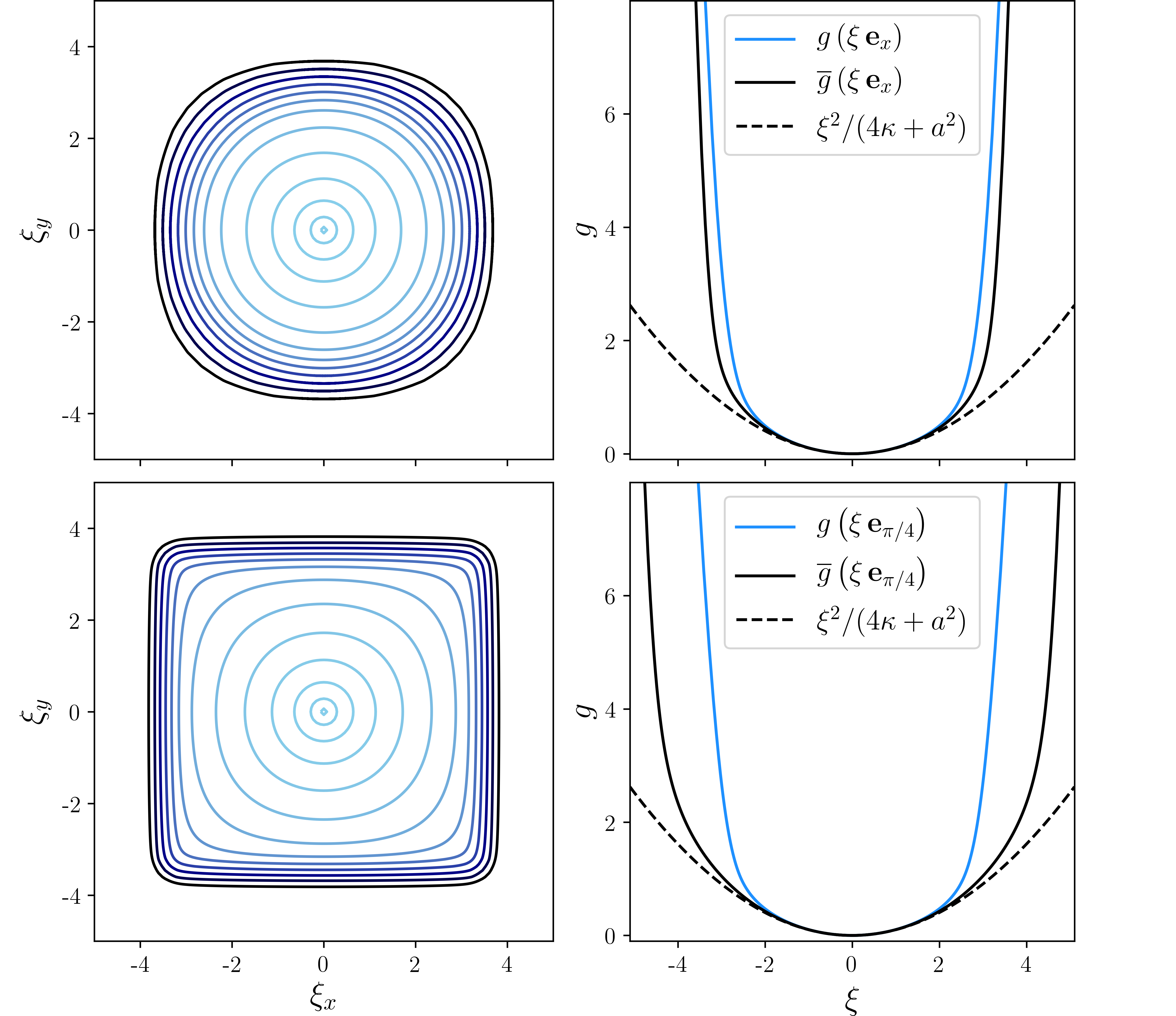
We show the results for the rate functions $g$ and $\overline{g}$, obtained from $f$ and $\overline{f}$ by numerical Legendre transform, in Fig. 4. The two functions are markedly different away from the centre ${\bm{\xi}}={\bm{\xi}}_{*}={\bm{0}}$ where the diffusion approximation applies and around which they are approximately equal. The function $g$ grows substantially faster than $\overline{g}$ (cf. Eq. (43)). Consequently, the ensemble-averaged $\mathbin{\langle C_{n}\rangle}$ considerably overestimates the tail concentration in single realisations of the flow. The departure from axis-symmetry, present for both $g$ and $\overline{g}$, is the result of the flow geometry: fast dispersion stems from particles experiencing maximum advection at each step, which can lead to the maximum displacements $(\pm a,\pm a)$ at each time step (ignoring diffusion). This indicates that for sufficiently large ${\bm{\xi}}$ (and sufficiently small $\kappa$), the contours of $g$ and $\overline{g}$ are approximately square as would be the case for advective displacements randomly chosen from $(\pm a,\pm a)$ at each iteration (A. Tzella and J. Vanneste 2016, cf.). This effect is much more marked for the ensemble-averaged concentration than for single realisations.

The broad conclusion is that the ensemble-averaged concentration is a poor predictor of the behaviour of dispersing passive scalars when it comes to their low-concentration tails. While the tail behaviour might seem of marginal interest, it plays a crucial role in the presence of chemical reactions, in particular by determining the dynamics of some reaction fronts. In this instance, the differences between single-realisation and ensemble-averaged dynamics can be dramatic as we discuss next.

We now consider the dynamics of a reacting scalar governed by the classical FKPP model of Fisher Fisher 1937 and Kolmogorov et al. Kolmogorov et al. 1937 which, in the presence of advection, reads

where $\gamma>0$ is the reaction rate and the concentration $C$ has been normalised so that its saturation value be $1$. According to this model, in an infinite domain, an initially localised patch of scalar spreads behind a reaction front.

For ${\bm{u}}=0$ and for $t\gg 1$, the front is circular in two dimensions (spherical in three) with a radius growing at the constant speed $s=2\sqrt{\kappa\gamma}$. For a spatially periodic flow, the front can be approximated by a self-similar convex curve (or surface) defined by

where $g$ is the large-deviation rate function introduced in (31) for the passive scalar problem (1) (i.e. $\gamma=0$ in (49)) (J. Gärtner and M. I. Freidlin 1979; Friedlin 1985; Xin 2000; A. Tzella and J. Vanneste 2014; A. Tzella and J. Vanneste 2015). The remarkable connection between the large-deviation tail of a passive scalar and the FKPP reaction front embodied by (50) can be understood heuristically as follows. The front’s propagation is controlled by its leading edge, where $C\ll 1$ so that (49) can be linearised about $C=0$; the solution is then that of the passive-scalar problem (1), approximately $\exp\left(-tg({\bm{x}}/t)\right)$, multiplied by the factor $\exp(\gamma t)$ associated with the (linearised) reaction, hence

Eq. (50) follows by observing that the front marks the transition between exponential growth and exponential decay.

For the random-in-time flows considered in this paper, $g$ is clearly the single-realisation rate function, so the shape of the front can be determined from (50) using that $g$ is the Legendre transform of the Lyapunov $f$ exponent of the random partial differential equation (38). The ensemble-averaged $\overline{g}$, while easier to evaluate, is only relevant to the front problem in the limit of small reaction rate $\gamma\ll 1$, when the diffusive approximation applies, $g\approx\overline{g}$, and the front is the ellipse (or ellipsoid)

as follows from Taylor expanding (50).

We illustrate how (50) predicts the shape of a reacting front by considering a reacting version of the alternating sine model (6). This adds the reaction step

where $C_{n+\frac{3}{4}}=\mathcal{K}*C_{n+\frac{1}{2}}$, to the advective and diffusive steps in (6), corresponding to the time-$1$ map associated with the FKPP reaction $\partial_{t}C=\gamma C(1-C)$. The front location is determined by the discrete-time equivalent of (50), that is,

Note that this equation makes it possible to interpret the contours of $g$ in Fig. 4 as giving the shape of fronts for different values of $\gamma$.

Figure 5 shows the concentration field obtained by direct numerical integration of the reacting alternating sine model starting from a localised patch with $a=\pi$, $\kappa=0.1$ and $\gamma=2$. The result is compared with the prediction (54) for the front location. The prediction which substitutes the ensemble averaged $\overline{g}$ (computed in subsection IV.2) is also shown. The figure confirms the validity of (54) and illustrates the inadequacy of the prediction based on $\overline{g}$.