Non-Markovian Noise Characterization with the Transfer Tensor Method
Abstract
We propose simple protocols for performing quantum noise spectroscopy based on the method of transfer tensor maps (TTM), [Phys. Rev. Lett. 112, 110401 (2014)]. The TTM approach is a systematic way to deduce the memory kernel of a time-nonlocal quantum master equation via quantum process tomography. With access to the memory kernel it is possible to (1) assess the non-Markovianity of a quantum process, (2) reconstruct the noise spectral density beyond pure dephasing models, and (3) investigate collective decoherence in multi-qubit devices. We illustrate the usefulness of TTM spectroscopy on the IBM Quantum Experience platform, and demonstrate that the qubits in the IBM device are subject to mild non-Markovian dissipation with spatial correlations.
I Introduction
Quantum information processing (QIP) is attracting increased attention from industry. As we enter the noisy intermediate-scale quantum (NISQ) era Preskill 2018, we face the near-term prospect of demonstrating non-trivial computations on quantum circuits consisting of 50-100 qubits without error correction. However, to sustain this level of engagement it is crucial to further improve the scale and achievable circuit depths of NISQ devices. At the core of this challenge is understanding the noise present in existing devices so that decoherence can be more effectively tamed Breuer and Petruccione 2007; de Vega and Alonso 2015; Breuer et al. 2016. In this work, we propose a method for quantum noise spectroscopy based on the tomographically reconstructed transfer tensor maps (TTMs) Cerrillo and Cao 2014 used in analyzing dissipative quantum dynamics. We demonstrate the utility of TTM noise spectroscopy by studying both simple theoretical models as well as IBM’s Quantum Experience (IBM Q) hardware on the cloud.
While quantum process tomography (QPT) Chuang and Nielsen 1997; Poyatos et al. 1997; Nielsen and Chuang 2000 has been widely adopted for experimentally characterizing quantum-gate fidelities Bialczak et al. 2010; Yamamoto et al. 2010; Rodionov et al. 2014 and environmental influences Yuen-Zhou et al. 2011; Howard et al. 2006, earlier theoretical and experimental efforts Kofman and Korotkov 2009; Howard et al. 2006 have largely been confined to analyzing noise under the Markovian assumption. Transfer tensor maps allow noise sources to be a comprehensively characterized by connecting experimentally deduced QPT data with the time-nonlocal quantum master equation (TNQME) Breuer and Petruccione 2007 valid for general open quantum systems,
| (1) |
where denotes the system’s reduced density matrix, is the Liouville superoperator corresponding to the system Hamiltonian, and is the memory kernel that fully encodes environment-induced decoherence effects. Through the tomographically reconstructed TTMs and translated memory kernel, experimentalists can more easily (1) characterize the non-Markovianity of a quantum process, (2) determine the noise power spectrum, and (3) estimate spatial and temporal correlations of nonlocal noise in multi-qubit systems. Furthermore, the TTM method facilitates noise characterization beyond pure dephasing models and works without having to implicitly assume the quantum or classical nature of the noise.
While the TTM method Cerrillo and Cao 2014; Buser et al. 2017; Kananenka et al. 2016; Gelzinis et al. 2017; Pollock and Modi 2018 can model arbitrary noise, we will largely be concerned with stationary Gaussian noise, which can be fully characterized by two-time correlation functions and noise spectral density. With the exception of a few special cases such as highly anharmonic spin baths Prokof’ev and Stamp 2000; Ma et al. 2015, this is a reasonable assumption. For instance, a spin bath surrounding a gated semiconductor quantum dot Hsieh et al. 2012 can often be modelled as classical Gaussian noise Hsieh and Cao 2018; Merkulov et al. 2002; Erlingsson and Nazarov 2002; Witzel et al. 2014. Also, the noise we observe often represents the overall effect of a system’s interactions with many background excitations. At the level of interacting with a single excitation, the coupling strength is often very weak. However, the cumulative effect (due to many background excitations) of the noise can be strong and may dominate the open system dynamics. In this scenario Makri 1999; Caldeira and Leggett 1983, our assumptions on the noise properties should hold.
It is instructive to compare TTM noise spectroscopy to another popular approach based on dynamical decoupling (DD) Viola and Lloyd 1998; Khodjasteh and Lidar 2005; Khodjasteh et al. 2010; Yang et al. 2011; Szankowski et al. 2017, which is an open-loop quantum control technique using -pulses (at a frequency much higher than the characteristic time scale of the noise) in rapid succession such that qubits become effectively isolated from their environment. While DD spectroscopy Álvarez and Suter 2011; Zwick et al. 2016; Norris et al. 2016; Paz-Silva et al. 2017 has recently been widely adopted to acquire noise statistics for quantum devices, results have largely been restricted to spin-based quantum circuits as the spectroscopy is based on the assumption that pure dephasing is the dominant decoherence mechanism Álvarez and Suter 2011; Zwick et al. 2016; Norris et al. 2016; Paz-Silva et al. 2017; Krzywda et al. 2018; Cywinski 2014; Yuge et al. 2011; Ma and Liu 2016. This assumption is incompatible with certain types of physical qubits, such as superconducting qubits which have extremely long coherence times Paik et al. 2011; Rigetti et al. 2012; Chen et al. 2014 in comparison to the gating times and which have comparable and time scales. Secondly, the repeated use of -pulse can potentially introduce adversarial effectsShiokawa and Lidar 2004 if the pulses are not in actuality fast relative to the cut-off frequency of the noise spectral density. We shall demonstrate that the TTM approach can not only reconstruct the noise power spectrum beyond pure dephasing models but can also achieve noise characterization without the need for a series of -pulses.
In multi-qubit circuits additional complexity emerges. As most fault-tolerant schemes Lidar and Brun 2013 assume independent noise on each qubit, it is crucial to have a quantitative diagnosis of the spatial and temporal correlations of decoherence effects among qubits in the system. DD noise spectroscopy Zwick et al. 2016; Norris et al. 2016; Paz-Silva et al. 2017; Krzywda et al. 2018 has been extended to use multi-qubit registers as a probe to analyze spatial correlations of noise. Similar to the single qubit case, DD based correlated noise spectroscopy still primarily focuses on pure-dephasing models. Again, the advantages of single qubit TTM spectroscopy extends to the case of multi-qubit systems.
In principle, TTM spectroscopy can be systematically applied to an arbitrary number of qubits. However, due to experimental constraints of performing high-dimensional QPT, it is most feasible to consider TTM based noise characterization for a small number of entangled qubits. In particular, we will only discuss two-qubit TTM spectroscopy in this work. However, recent advances in adopting techniques such as compressed sensing Gross et al. 2010; Riofr√≠o et al. 2017 and variational ansätze derived from machine learning Torlai et al. 2018; Rocchetto et al. 2018; Torlai and Melko 2018 and matrix product states Cramer et al. 2010; Lanyon et al. 2017 have greatly improved the prospects of tomographic scalability. Additional efforts, such as using machine learning Palmieri et al. to tame state preparation and measurement errors, without resorting to expensive gate set tomography and similar techniques Merkel et al. 2013; Blume-Kohout et al. 2013, could further strengthen the attractiveness of TTM noise spectroscopy in comparison to other well-established approaches in the near future.
The remainder of this work is organized as follows. Sec. II contains an introduction to transfer tensor maps. Sec. III discusses the proposed TTM noise spectroscopy. Sec. IV describes the usage of TTM noise spectroscopy with examples based on theoretical models. Sec. V summarizes a testing of the TTM method on IBM’s Quantum Experience hardware. Section VI concludes.
II Transfer tensor maps
We first recall the essential theoretical background of TTM as originally formulated in Ref. Cerrillo and Cao 2014. In this work, we are concerned with a collection of qubits governed by the following Hamiltonian,
| (2) | |||||
where is a time-independent system Hamiltonian for the qubits, and describes the system-noise coupling. is a Pauli operator with the index labeling the qubits and the index one of the Cartesian components. is a bath operator explained below. Let us clarify the distinction between quantum and classical noise defined in this work. When the environment consists of quantum systems, is a bath operator in the interaction picture with respect to , the environment Hamiltonian. When the environment consists of classical stochastic baths, are real-valued stochastic processes. In both cases, we only consider Gaussian noise, which is fully characterized by the first two statistical moments and .
Furthermore, we assume an initial state of the qubits to be independent of the environment. Time evolution for an open quantum system can be cast in the following form,
| (3) | |||||
where the subscript on the exponential functions denotes the (anti-)chronological time ordering of the time-evolution operator and is the dynamical map relating the time-evolved reduced density matrix back to the initial state. The bracket denotes an average over the environmental degrees of freedom. Experimentally, the dynamical maps for a -level quantum state are derived from an ensemble of QPTs obtained under different initial conditions.
The QPTs are performed at equidistant time intervals, i.e. , and we may write . Transfer tensors are then defined by
| (4) |
with . Replacing the dynamical maps in Eq. (3) with in Eq. (4), one obtains
| (5) |
Equation (5) shows that the dynamical evolution up to time depends on the system’s history in the presence of noise. The TTM encodes how much the system’s state at an earlier time contributes to the formation of the current state . A time translational invariance is implied for the transfer tensor maps in Eq. (5) as they are labeled by the time difference between the two density matrices and . Equation (5) holds as we only consider time-independent . In general, the dynamical evolution should only significantly depend on the system’s history up to certain point. This implies that one may accurately estimate the quantum dissipative dynamics when the the summation in Eq. (5) is truncated at large enough index , drop all summands for time . This theoretical insight has an important consequence for experiment: one only needs to perform QPTs up to time . Beyond , all quantum dynamical information can be recursively determined via Eq. (5).
III TTM based Noise Spectroscopy
When the time increment is small, Eq. (5) essentially prescribes a numerical solution to Eq. (1) with the identification
| (6) |
with the Kronecker delta function. The translated memory kernel of the TNQME, Eq. (1), is the foundation of the noise spectroscopy method to be explicated in this section.
III.1 A measure of non-Markovianity
Transfer tensor maps can be used to gauge the non-Markovianity of a quantum dynamical process. A simple argument is as follows Cerrillo and Cao 2014. A Markovian process requires only the present state to determine the next state, i.e. for all . Hence, there should be only one non-trivial transfer tensor (i.e. the Frobenius norm for ) for any . Whenever multiple transfer tensors are needed to accurately approximate Eq. (5) the environment can be qualitatively argued as being non-Markovian. Alternatively, recall that the transfer tensors (stored as matrices) encode the memory kernel for in Eq. (6) when is small. The temporal profile of the memory kernel, another qualitative indicator of non-Markovianity, can be gauged by the norm of TTM matrices constructed at different time points.
Counting the number of TTMs with sizable norm, however, does not fully capture the multifaceted nature of a non-Markvoian quantum process Breuer et al. 2016; Rivas et al. 2014; Pollock et al. 2018. Transfer tensor maps may be used though, in combination with advanced theory of open quantum systems, to construct a variety of more insightful non-Markovianity measures. As an example, consider the Bloch volume measure Lorenzo et al. 2013 put forward by Lorenzo, Plastina and Paternostro. This scheme uses the Bloch sphere representation of a qubit as
| (7) |
with the Bloch vector . Each Bloch vector component is determined via . In this geometric view of quantum dynamics, the action of on can be represented as an affine transformation on , i.e. . It is known that the volume of accessible states at time is a monotonically decreasing function for Markovian dynamics. The Bloch volume measure is then defined as
| (8) |
which accumulates the positive rate of change when the volume of accessible states increases due to deviations from Markovianity. Note that is not a comprehensive non-Markovian measure as it is insensitive to non-Markovianity associated with the vector. Nevertheless, it is one of the simplest measures to evaluate that still gives insight into the underlying dynamical process.
A few toy models aside, evaluating Eq. (8) requires tracking the time-dependent dynamical maps in order to observe the temporary reversal of the volume contractions and information backflow for non-Markovian processes in an experimental setting. By a straightforward modification of Eq. (5), we arrive at a recursive relation . This relation significantly reduces the number of required QPTs when one attempts to experimentally evaluate Eq. (8), because one can re-use a small number of QPTs (up to time ) to numerically generate addition dynamical maps at .
III.2 Noise spectral density: weak noise-coupling
For simplicity, we explain how to construct the noise spectral density for a single qubit coupled to quantum noise. Extension of the this method to the two-qubit case is straightforward. Furthermore, in App. A we show that the the case of classical noise may also be dealt with using only minor modifications. The weak-coupling (to noise sources) implies that it is sufficient to approximate the memory kernel with the leading order term of a perturbative expansion with respect to .
The exact memory kernel for an arbitrary quantum bath can be written as follows,
| (9) |
where projection operators and are defined by , i.e. projects a system-bath entangled quantum state to a factorized form consisting of a system part , and a bath part which is a stationary state with respect to the bath Hamiltonian defined in Eq. (2). We note that the kernel is a stationary process when the noise satisfies the stationary Gaussian conditions.
We first discuss TTM noise spectroscopy in the weak noise-coupling regime, which may be a reasonable approximation for high quality qubits well protected from noise, using a second-order perturbative treatment of the memory kernel. The general case will follow in the next section.
The memory kernel for Gaussian noise can be expressed as , where corresponds to the order expansion of the Hamiltonian with respect to . Keeping only the leading (i.e. second order) term gives
| (10) | |||
where and the bath correlation function is given by
| (11) |
We suppress the index on Pauli matrices and noise operators as we only consider one qubit here. Since the TTM matrices and the memory kernel are related via Eq. (6), every experimentally determined TTM matrix element is a linear combination of 9 correlation functions, , when the second-order perturbation, Eq. (10), holds. To numerically process the data and determine the correlation functions, we resort to solving a sequence of optimization problems,
| (12) | |||||
where is the experimentally determined memory kernel. We numerically identify a set of to minimize the difference between the theoretically constructed second-order memory kernel matrix and the experimentally obtained memory kernel matrix at . Subsequently, we determine the numerical values of the correlation functions at by solving the same minimization problem with an additional regularization enforcing the continuity of the correlation functions with hyperparameters .
Once the noise correlation function is determined, the corresponding spectral density can be determined by invoking the fluctuation-dissipation theorem Yan and RuiXue 2005, which gives
| (13) |
The positivity of for is ensured if , the Fourier transform of , is positive.
Throughout this derivation, we do not make any assumption of a pure dephasing model. This makes TTM noise spectroscopy particularly suitable for superconducting qubits as further detailed in Sec. V.
III.3 Noise spectral density: beyond weak coupling
Beyond the weak-coupling limit, one must retain more terms in the expansion of the memory kernel, . It is thus more tedious to infer the correlation functions from the TTM matrix elements. To overcome this challenge, we propose to tomographically reconstruct a family of memory kernels under different conditions. The -th case is distinguished from other cases by , the system’s characteristic energy scale of . After casting each in its characteristic time scale , the second-order memory kernel for the original problem can be extracted from linear combinations of the scaled , and one may follow the numerical recipe introduced in Sec. III.2 to recover the correlation functions and the associated spectral density.
We rely on several assumptions. First, we take the system Hamiltonian to be , a simple bias. Second, the qubit’s characteristic energy scale, can be freely adjusted over a certain range , which is a reasonable assumption for tunable quantum devices. Third, the adjustment of should not alter the noise source. These requirements are compatible with many physical systems. For instance, a recent experimentHernandez-Gomez et al. 2018 on spin-based qubits in NV center fulfills these requirements.
The procedure goes as follows. For a chosen energy bias , the quantum dynamics is governed by the Hamiltonian . If a time unit of is adopted, then the dimensionless Hamiltonian reads with . By performing such experiments with distinct energy biases with , one may construct a set of dimensionless memory kernels, which are related by
| (14) |
where and denotes the -th order term of the memory kernel for an energy bias . If we assign the original case of interest as the case, then we may define a matrix,
which encodes the linear algebraic relation . By converting the matrix into a lower triangular form, one learns how to linearly combine to recover , which is accurate up to the -th order perturbative truncation of the memory kernel stated in the beginning of this section. Finally, is recovered when one reverts back to the original time unit scale.
III.4 Two-qubit environment spectroscopy
In a two-qubit circuit, unintentional entanglement between the qubits may be built up when the qubits share a common noise source. It is thus desirable to unravel the two-qubit TTMs into single-qubit and two-qubit contributions so that one may not only detect the presence of common noise but also determine a quantitative estimate of its contribution to collective deocherence.
First, we write two-qubit dynamical maps in the basis of tensor products of single-qubit basis. In the such a basis, two-qubit dynamical maps may be rigorously decomposed as
| (20) | |||||
where and are the reduced dynamical maps after tracing out the system 2 and system 1, respectively. Details of this decomposition of bipartite dynamical maps are given in App. B. If the two qubits are not directly coupled, then the dynamical maps can be exactly separated with for all . In some earlier works Kofman and Korotkov 2009, is directly used to diagnose collective decoherence.
The decomposition of into a separable component and correlated component is particularly useful when second-order perturbation theory holds. This is assumed for our analysis of two-qubit systems subsequently discussed in Sec. IV.2 and V.2, respectively. Whenever the observed dynamical process falls beyond this perturbative regime, one may find to be comparable to or even dominate . This implies the physical picture of having two localized quantum subsystems is no longer an appropriate basis to discuss a strongly correlated quantum system.
A similar set of separable and correlated tensor maps may also be defined as
| (21) | |||||
| (22) |
with , and the correlated memory kernel identified as
| (23) |
The Liouville superoperator reveals whether a direct qubit-qubit coupling term , unrelated to the noise, is present in the qubit Hamiltonian . It is beneficial to identify the main cause of collective decoherence, and devise a corresponding strategy to improve the coherence of the quantum hardware. If one simply looks at the dynamical map , it is hard to distinguish the source of collective decoherences: (1) a direct coupling , (2) genuine correlated noises, or (3) an interplay of both factors. To complicate the situation, two entangled qubits suffer collective decoherence even when they are subjected to independent noise with .
In pure dephasing models, it is possible to quantitatively distinguish between the contributions of the two factors. An unintentional coupling will give rise to the term in (23) only and nothing else. On the other hand, effects of correlated noise sources are exclusively encoded in the correlated part of the memory kernel. In more general decoherence models, both factors contribute to the correlated memory kernel. Nevertheless, still only encodes the effects given by . We may estimate the term by performing short-time QPT at 2 different time step size and . Linear combinations of the two different maps, and , can be used to isolate the two terms as and scale as and , respectively. This analysis therefore still provides a gauge on the relative importance of the two factors for collective decoherence.
IV TTM spectroscopy on theoretical models
We first illustrate the usefulness of TTM spectroscopy through numerical experiments, using real-valued Gaussian random noise. As we shall see, the numerically processed TTM data reveals much about the noise properties.
IV.1 One-Qubit Case
We first consider a one-qubit pure phasing model, which is commonly used to illustrate DD spectroscopy. The Hamiltonian reads and . The noise satisfy the statistical moments: and . For these cosine functions modulated with an exponentially decaying envelope, the corresponding spectral density has the Lorentzian profile.
The pure dephasing dynamical maps are given by
with
| (29) |
Note that these dynamical maps satisfy as required. It is straightforward to verify that these maps are not divisible, i.e. for this pure-dephasing model; hence, the dynamics is clearly non-Markovian.

In the upper panel of Fig. 1 we plot the norms of different TTM matrices. and note that more than one TTM matrix has sizable norm. This observation confirms the non-Markovianity of the dynamical process is positively correlated with TTM norm distribution. Furthermore, the norms of higher order matrices are increasingly suppressed, justifying the earlier claim that we should be able to truncate Eq. (4) to include only the first few TTMs with non-trivial norms when we make dynamical predictions based on Eq. (5). In the lower panel of Fig. 1 we plot the norm of the off-diagonal matrix element, , as a function of time. The curve with black circles is the exact result , which requires explicitly evaluating the integral in Eq. (29) at every time point. The other curves are results obtained by using different numbers of TTMs in the way prescribed by Eq. (5) to predict quantum dynamical evolution. In this case, we consider using the first TTMs, respectively. Accurate results are obtained for the entire simulation duration when a sufficient number () of TTMs are taken into account.

Next we analyze the non-Markovianity of the dynamical process by plotting the Bloch volume measure in Fig. (2). One sees the signature of non-Markovianity manifested in the temporary increase of the Bloch volume. This increase happens around the time interval spanned by , and in the figure. The exact result and TTM prediction (based on first 5 data points) agree very well across the entire simulation time window. This is an encouraging indication that TTM may facilitate the implementation of theoretical non-Markovianity measures in an experiment.
A critical role of a quantum noise spectroscopy is determining the noise spectral density. Since the spectral density is the Fourier transform of a correlation function, we will be content if we obtain the noise correlation function. First, we consider the case of weakly coupled noise where the approximation is valid. We use the numerical method, Eq. (12), proposed in Sec. III.2 to infer the correlation function. In the upper panel of Fig. (3), we plot the numerically recovered correlation function based on TTM data, and it agrees well with the theoretical correlation function that the random noise must satisfy in our numerical experiment. We next explore a broader range of system-noise coupling strength. It is no longer valid to assume in the stronger coupling regime. For simplicity, we consider noise coupling just strong enough that the memory kernel can be well approximated by . We follow the prescription in Sec. III.3 to first extract the second-order memory kernel by using two sets of simulations under different . In the lower panel of Fig. (3), we plot the the theoretical and numerical values of the correlation functions at a specific time point versus the noise coupling strength. One clearly sees the increasing deviation of the numerically recovered correlation functions obtained under the second-order approximation as the noise coupling strength increases. However, the correct correlation function can still be recovered when we apply the method of Sec. III.3.

Lastly, we present a model with population relaxation in order to demonstrate the wide applicability of TTM noise spectroscopy. The Hamiltonian we consider is and . As shown in Fig. (4), TTM noise spectroscopy also accurately reproduces the theoretical results for a non-pure-dephasing model, without requiring adjustments to the procedure.

IV.2 Two-Qubit Case
We now turn to two-qubit spectroscopy, and consider two different models for comparison. In the first case, two coupled qubits are subject to independent noise, and . In the other case, the qubits are not directly coupled but are subject to correlated noise, with . We shall refer to these as the independent (first) and correlated (second) models, respectively.

In Fig. (5), we plot the norms of the full, separable, and correlated TTMs (i.e. , , and , respectively) for the first model in the upper panel and the second model in the lower panel. For better presentation, we subtract an identity matrix from and plotted in both panels of Fig. (5). In the upper panel, only has non-trivial norm. This result indicates that the correlated part of the TTM is “almost” Markovian in nature when two qubits are subject to independent noise. One can further decompose into and . This can be done because the definition implies the two terms scale differently with respect to . Hence, we can construct two (with slightly different time step size ), and simple algebraic manipulations allow us to isolate the individual terms, or , making up . In this particular case, we confirm (cf. App.C) that the , reminiscent of the term, is responsible for entangling the two qubits and allows decoherence effects to be correlated even if the noise sources are spatially separated and independent. In the second case (with explicitly correlated noise), we plot the norms of different TTMs in the lower panel of Fig. (5). Here, multiple have sizable norm. A closer inspection on the magnitude of and indicates that is the main contributing factor for . Based on this straightforward analysis of TTM norm distribution, one can estimate the relative importance of different physical mechanisms contributing to collective decoherence.

We next investigate the set of correlated TTMs . Figure (6) presents the dynamical evolution of an off-diagonal matrix elements of a two-qubit density matrix. Similar to the single-qubit case in Fig. (1), we compare the dynamics generated via TTM with the exactly simulated results. Across the upper panel, we plot the dynamical prediction based on the full TTM (left column) and separable TTM (right column) against the exact results for the first model. Across the lower panel, we compare the results of full TTM (left column) and separable TTM (right column) to the exact results for the second model. In both cases, effects of collective decoherence are seen by the failure to correctly generate the dynamics using the separable TTM alone. One may be deceived by Fig. (5) into thinking that might not play important roles in both two models we consider here, as the norms for are much smaller to those of . Yet, dropping these seemingly small terms results in inaccurate dynamical predictions as shown by the discrepancy between the left and right columns of Fig. (6). This observation exemplifies the intricate nature of highly non-Markovian dynamics. The norm distribution of the full TTMs in both panels of Fig. (5) suggests high non-Markovianity in both cases we investigate.
The model studies in this section illustrate the usefulness of using TTM spectroscopy to distinguish between the underlying causes of collective decoherences in multi-qubit circuits. Improving the coherence time would require very different engineering efforts to either reduce a direct qubit-qubit interaction, , or to eliminate common noise sources.
V TTM on the IBM Quantum Experience
We further test TTM spectroscopy on IBM’s 14-qubit device, “IBM Q Melbourne”. In this device, a single-qubit pulse lasts 100 with a buffer time of 10 free evolution between pulses. To construct the TTMs, we apply a sequence of ‘identity’ gates to instruct the control system not to interfere with the qubit’s free evolution in the presence of noise sources. Because of the aforementioned setup for this particular device, we always sample the QPTs at integer multiples of 110 , the combined time for a single-qubit rotation and an interim buffer.
To obtain QPTs, we perform all possible n-qubit Pauli measurements under initial conditions at every sampling time point. We denote with , the identity operator. We perform simple tests to demonstrate that TTM provides numerous insights to characterize noise properties even when only restrictive operations performed over the cloud are possible. Additional details may be found in App. D.
V.1 One-Qubit Case

We first convert the experimental QPTs collected from an IBM device into TTMs. The norm distribution is displayed in the upper panel of Fig. (7). We find the qubits are affected by non-Markovian noise, as there is more than one TTM with sizable norm in the plot.

We next perform additional experiments to corroborate the usefulness of TTMs. First, we use to predict the dissipative quantum dynamics. As inferred from the upper panel of Fig. (7), a minimum of 3 TTMs is required to faithfully reproduce the dissipative effects arising from noise influences. In the lower panel, we do observe that significant errors accumulate quickly when fewer TTMs are used. Figure (7) suggest the memory kernel’s time length lasts on the order of 1 s. This is not particularly short in comparison to the gating time of 100 ns.
We further investigate other aspects of non-Markovianity by plotting the Bloch volume in Fig. (8). In this case, the temporary reversal of the Bloch volume contraction (inset of Fig. (8)), is observed far outside the time window for data acquisition. The first five data points in Fig. (8) are experimentally measured results from the IBM device, the rest are numerically generated with the help of TTMs. Without relying on TTM predictions, it is not possible to obtain such a result given the circuit depth restriction on the IBM Q. While we do observe a signature of non-Markovianity, the magnitude of the Bloch volume is already very small, as shown in the inset of Fig. (8). Hence, the observed reversal of Bloch volume contraction does not imply a strong degree of non-Markovianity.

Next, we draw attention to a recent work Pokharel et al. 2018 by Pokharel et. al. to study the effects of DD on preserving qubit coherence on both IBM and Rigetti devices. They use the DD control scheme to prolong qubit coherence. We repeat the DD experiment as shown in in Fig. (9), and verify the prolonging of quantum coherence and the trapping of state populations. This change in the underlying dynamical process is reflected in the effective TTM norm distributed plotted in (10). We note that the effective noise under DD control scheme looks more Markovian with a sharper decay profile in the norm distribution in comparison to the original one (free evolution) given in Fig. (7). This is consistent with the observation given by Pokharel et. al.

V.2 Two-Qubit Case
In two-qubit circuits we are primarily interested in detecting spatially correlated noise sources and their contributions decoherence, cf. the circuit layout in Fig. (13). To this end, we plot the norms of full TTMs (), separable TTMs () and correlated TTMs (). Due to larger state preparation errors arising from the use of two-qubit gates, the TTM norm distribution stabilizes at a value much higher than 0 in Fig. (11) in comparison to the one-qubit results given in Fig. (7). Nevertheless, the norm profile of first few TTMs suggest that correlated noise can play a significant role in the overall decoherence for the two-qubit circuit.


To vindicate this hypothesis, we check the dynamics inferred from the full and separable TTMs, respectively, against the experimental data shown in Fig. (12). The time evolution of a separable initial state, upper row in Fig. (12), is noticeably influenced by the collective decoherence because panel a (full TTM) and b (separable TTM) give inconsistent results. For an initially unentangled two-qubit system, there should not be any entanglement generation when being left alone as in this experiment. Yet, the strong disagreement between predictions by full and separable TTMs indicate that the two qubits must be subsequently entangled due to the action of . We also look at the concurrence for the two-qubit density matrix (directly obtained from state tomography) as an additional check to confirm the emergence of non-trivial entanglement after the state preparation stage at . Unsurprisingly, the time evolution of an initially entangled state, lower row of Fig. (12), is also influenced by the collective decoherence as panel c (full TTM) and d (separable TTM) yield inconsistent outcomes. In both cases, actually help to sustain quantum coherence.
To identify the source of collective decoherence in this circuit, we perform the analysis discussed in App. (C), i.e. we isolate and from and compare their norms. We find both terms to be non-negligible with slightly dominant. Efforts to minimize the presence of collective noise () and suppression of cross-talk () are thus both needed to improve coherence on this particular device.
VI Conclusion
In this work, we proposed transfer tensor map based noise spectroscopy that enables physicists and engineers to more easily (1) characterize the non-Markovianity of a noise source, (2) determine the noise power spectrum, and (3) estimate spatial and temporal correlations of nonlocal noise a multi-qubit systems. In addition, the TTM spectroscopy facilitates noise characterization beyond pure dephasing models.
The key idea is to tomographically reconstruct the well-established TNMQE with a memory kernel that encodes all information required to predict the effects of the noise. Furthermore, the second-order memory kernel is known to be proportional to the noise’s autocorrelation functions. For high-quality quantum computing hardware, qubits should be weakly coupled to noise. Therefore, one may often assume and deduce the correlation functions according to Eq. (12). The noise power spectrum can be subsequently generated. For non-weak-coupling cases, we propose a simple remedy to perform a series of experiments to extract the desired noise’s correlation function in Sec. III.3. Furthermore, we discuss how to unravel two-qubit TTMs to investigate the underlying nature of collective decoherence.
To illustrate different aspects of the proposed TTM spectroscopy, we applied it to simple theoretical models as well as IBM Q’s hardware. For theoretical models, we demonstrated an efficient scheme to assess the non-Markovianity of a quantum process, reconstructed the noise’s correlation functions and clarified the source of collective decoherence for two-qubit circuits. For the IBM Q hardware, the predictive power of TTM spectroscopy was unambiguously demonstrated. This implies that the TTMs encode realistic decoherence effects on the qubits. We show that the qubits undergo non-Markovian dissipation. Finally, we observe that collective decoherence is due to the presence of spatially correlated noise sources as well as cross-talk between qubits in the “IBM Q Melbourne” device.
Appendix A Derivation of the Time-NonLocal Quantum Master Equation for Classical Noises
Given , the Hamiltonian in Eq. (2), we first consider the case of quantum noise. In this case, the projection is defined via
| (30) |
where is a joint system-bath quantum state and (the identity operator). By introducing the projectors and into the Liouville equation for the joint system, we obtain
| (31) |
where . We note that the equation of motion for can be formally integrated. By substituting the formal solution of into the equation of motion for , one derives
| (32) | |||||
Furthermore, by assuming (consistent with properties of Gaussian noise) and (a factorized initial state of the form ) the above equation reduces to the TNQME, Eq. (1) with the memory kernel given in Eq. (9).
Next, we consider the case of classical noise. In this case, the system is not explicitly coupled to another quantum system acting as a source of noise. Rather, the system is subjected to classical noise sources with the Hamiltonian parameterized by Gaussian stochastic process . In this case, we define the projector via
| (33) |
where denotes an average over the Gaussian noise sources, while is a stochastic instance of the system’s density matrix. Similarly, the complementary projector satisfy the relation . By going through mathematical manipulation for the quantum-noise case, one derives
| (34) | |||||
where . Similarly, one has to make the same assumptions: and ; then one obtains formally the same TNQME, Eq. (1) with a structurally identical memory kernel. The subtle differences between quantum and classical cases are as follows. (1) is a stochastic superoperator acting on the system in the classical case, while in the quantum setting it is a deterministic superoperator acting on the joint system and bath Hilbert space; and (2) The definitions of the projection operator differ in Eq. (30) and (33).
Finally, to obtain the spectral density for the classical noise case, note that the second-order memory kernel retains the functional form of Eq. (10) with the obvious condition that has to be strictly real-valued and . In this case, the noise spectral density is obtained via the Wiener-Khinchin theorem Clerk et al. 2010 for stochastic processes,
| (35) |
The spectral density obeys for classical noise.
Appendix B Matrix Representations of Dynamical Maps
In Sec. III.3, we implicitly assume the following matrix form Shen et al. 2017 for a dynamical map ,
| (36) |
where , and refers to one of the orthogonal set of quantum states for a -level quantum system. The state transformation induced by the superoperator (of dimension by ) can be operationally carried out as a matrix vector product when the density matrix is encoded as a vector of length in a Liouville space, i.e. . The structural form of brings many operational advantages. For instance, a successive transition (in the form of compositions of dynamical maps) can be done with simple matrix multiplications, .
However, the Choi matrix Caruso et al. 2014; Filippov et al. 2017, an alternative representation of the dynamical process, possesses other advantages. In order for a Choi matrix to represent a valid dynamical map, the matrix has to satisfy the trace condition (sum up to dimension of the Hilbert space), positivity, and Hermiticity. The Choi matrix is defined via,
| (37) |
where the operators . The the matrices defined in Eq. (36) and (37) are related via
| (38) |
For a bipartite quantum system (composed of two -level subsystems), the common practice is to index the state as with and the Liouville-space basis element via . For this study, we find it is useful to re-index the Liouville-space basis element by replacing the standard approach with , where and ,,, . In terms of re-indexed Liouville-space basis elements, we get a convenient form of separable quantum channels for a bipartite system,
| (39) |
If we define , i.e. , then we can recover the individual Choi matrices, such as and vice versa.
For a general bipartite quantum dynamical process, we can write any Choi matrix as , where . The correlated term vanishes exactly for separable quantum channels. Based on Eq. (38), we can re-arrange the matrix elements of various matrices to obtain the corresponding matrices. In particular, the factorized dynamical map reads,
| (40) | |||||
Appendix C TTM Spectroscopy on Two-qubit Theoretical Models
To isolate the and terms, we construct two with different time step sizes and , respectively. This gives
| (41) |
Since is small ( the correlation length of noise ), we take . This approximation leads to
| (42) |
By substituting the transfer tensors and obtained for the first model (coupled qubits subjected to independent noises) in Sec. IV.2 into Eqs. (C), we find
| (43) | |||||
which agrees well with the theoretical results of as
Similarly, if we substitute and for the second model (independent qubits subjected to correlated noises) into Eqs. (C), we find
| (44) | |||||
which agree well with the theoretical results for a correlated noise kernel as .
As commented at the end of Sec. III.3, one can very accurately unravel the underlying causes for a collective decoherence in a multi-qubit circuit by following the analysis on the correlated transfer tensor maps outlined in this appendix.
Appendix D Quantum Process Tomography on the IBM Quantum Experience
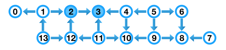
The experiments reported in Sec. V were performed on a 14-qubit chip. The connectivity between qubits is illustrated in Fig. (13). Below, we briefly describe the set of quantum states used to obtain dynamical maps via QPT.
Dynamical maps are a linear, completely positive, trace preserving transformations. Quantum process tomography (QPT) is the protocol to determine the dynamical map evolving a general state from one point in time to another. This procedure requires one to perform a series of experiments involving various combinations of initial states and measurements. If the system under consideration has dimension d, we may choose pure sates for the QPT reconstruction. For an one-qubit system, we prepare the following four states as the basis for
experiments run on the IBM Q:
| (45) |
For a two-qubit system, we choose the following sixteen states as the basis:
| (46) | |||||
We note the dynamical maps introduced in Sec. II are matrices with respect to the standard basis where for (one-qubit case) or (two-qubit case). Because quantum dynamical processes are linear maps, it is straightforward to convert the experimentally reconstructed QPTs into dynamical maps in the standard basis.
References
- Preskill (2018) J. Preskill, Quantum 2, 79 (2018).
- Breuer and Petruccione (2007) H.-P. Breuer and F. Petruccione, The Theory of Open Quantum Systems (Oxford University Press, 2007).
- de Vega and Alonso (2015) I. de Vega and D. Alonso, Rev. Mod. Phys. 89, 015001 (2015).
- Breuer et al. (2016) H.-P. Breuer, E.-M. Laine, J. Piilo, and B. Vacchini, Rev. Mod. Phys 88 (2016).
- Cerrillo and Cao (2014) J. Cerrillo and J. Cao, Phys. Rev. Lett. 112, 110401 (2014).
- Chuang and Nielsen (1997) I. L. Chuang and M. A. Nielsen, J. Mod. Opt. 44, 2455 (1997).
- Poyatos et al. (1997) J. F. Poyatos, J. I. Cirac, and P. Zoller, Phys. Rev. Lett. 78, 390 (1997).
- Nielsen and Chuang (2000) M. A. Nielsen and I. L. Chuang, Quantum computation and quantum information (Cambridge University Press, Cambridge, England, 2000).
- Bialczak et al. (2010) R. C. Bialczak, M. Ansmann, M. Hofheinz, E. Lucero, M. Neeley, A. D. O’Connell, D. Sank, H. Wang, J. Wenner, M. Steffen, A. N. Cleland, and J. M. Martinis, Nat. Phys. 6, 409 (2010).
- Yamamoto et al. (2010) T. Yamamoto, M. Neeley, E. Lucero, R. C. Bialczak, J. Kelly, M. Lenander, M. Mariantoni, A. D. O’Connell, D. Sank, H. Wang, M. Weides, J. Wenner, Y. Yin, A. N. Cleland, and J. M. Martinis, Phys. Rev. B 82, 184515 (2010).
- Rodionov et al. (2014) A. V. Rodionov, A. Veitia, R. Barends, J. Kelly, D. Sank, J. Wenner, J. M. Martinis, R. L. Kosut, and A. N. Korotkov, Phys. Rev. B 90, 144504 (2014).
- Yuen-Zhou et al. (2011) J. Yuen-Zhou, J. J. Krich, M. Mohseni, and A. Aspuru-Guzik, Proc. Natl. Acad. Sci. 108, 17615 (2011).
- Howard et al. (2006) M. Howard, J. Twamley, C. Wittmann, T. Gaebel, F. Jelezko, and J. Wrachtrup, New J. Phys. 8, 33 (2006).
- Kofman and Korotkov (2009) A. G. Kofman and A. N. Korotkov, Phys. Rev. A 80, 042103 (2009).
- Buser et al. (2017) M. Buser, J. Cerrillo, G. Schaller, and J. Cao, Phys. Rev. A 96, 062122 (2017).
- Kananenka et al. (2016) A. A. Kananenka, C.-Y. Hsieh, J. Cao, and E. Geva, J. Phys. Chem. Lett. 7, 4809 (2016).
- Gelzinis et al. (2017) A. Gelzinis, E. Rybakovas, and L. Valkunas, J. Chem. Phys. 147, 234108 (2017).
- Pollock and Modi (2018) F. A. Pollock and K. Modi, Quantum 2 (2018).
- Prokof’ev and Stamp (2000) N. Prokof’ev and P. Stamp, Rep. Prog. Phys. 63, 669 (2000).
- Ma et al. (2015) W.-L. Ma, G. Wolfowicz, S.-S. Li, J. J. L. Morton, and R.-B. Liu, Phys. Rev. B 92, 161403 (2015).
- Hsieh et al. (2012) C.-Y. Hsieh, Y.-P. Shim, M. Korkusinski, and P. Hawrylak, Rep. Prog. Phys. 75, 114501 (2012).
- Hsieh and Cao (2018) C.-Y. Hsieh and J. Cao, J. Chem. Phys. 148, 014104 (2018).
- Merkulov et al. (2002) I. A. Merkulov, A. L. Efros, and M. Rosen, Phys. Rev. B 65, 205309 (2002).
- Erlingsson and Nazarov (2002) S. I. Erlingsson and Y. V. Nazarov, Phys. Rev. B 66 (2002).
- Witzel et al. (2014) W. M. Witzel, K. Young, and S. Das Sarma, Phys. Rev. B 90, 115431 (2014).
- Makri (1999) N. Makri, J. Phys. Chem. B 103, 2823 (1999).
- Caldeira and Leggett (1983) A. Caldeira and A. J. Leggett, Ann. Phys. 149, 374 (1983).
- Viola and Lloyd (1998) L. Viola and S. Lloyd, Phys. Rev. A 58, 2733 (1998).
- Khodjasteh and Lidar (2005) K. Khodjasteh and D. Lidar, Phys. Rev. Lett. 95, 180501 (2005).
- Khodjasteh et al. (2010) K. Khodjasteh, D. A. Lidar, and L. Viola, Phys. Rev. Lett. 104, 090501 (2010).
- Yang et al. (2011) W. Yang, Z.-Y. Wang, and R.-B. Liu, Front. Phys. 6, 2 (2011).
- Szankowski et al. (2017) P. Szankowski, G. Ramon, J. Krzywda, D. Kwiatkowski, and L. Cywinski, J. Phys.: Condens. Matter 29, 333001 (2017).
- Álvarez and Suter (2011) G. A. Álvarez and D. Suter, Phys. Rev. Lett. 107, 230501 (2011).
- Zwick et al. (2016) A. Zwick, G. A. Alvarez, and G. Kurizki, Phys. Rev. Appl. 5, 014007 (2016).
- Norris et al. (2016) L. M. Norris, G. A. Paz-Silva, and L. Viola, Phys. Rev. Lett. 116, 150503 (2016).
- Paz-Silva et al. (2017) G. A. Paz-Silva, L. M. Norris, and L. Viola, Phys. Rev. A 95, 022121 (2017).
- Krzywda et al. (2018) J. Krzywda, P. Sza≈Ñkowski, and ≈. Cywi≈Ñski, arXiv:1809.02972 (2018).
- Cywinski (2014) L. Cywinski, Phys. Rev. A 90, 042307 (2014).
- Yuge et al. (2011) T. Yuge, S. Sasaki, and Y. Hirayama, Phys. Rev. Lett. 107, 170504 (2011).
- Ma and Liu (2016) W.-L. Ma and R.-B. Liu, Phys. Rev. Appl. 6, 054012 (2016).
- Paik et al. (2011) H. Paik, D. I. Schuster, L. S. Bishop, G. Kirchmair, G. Catelani, A. P. Sears, B. R. Johnson, M. J. Reagor, L. Frunzio, L. I. Glazman, S. M. Girvin, M. H. Devoret, and R. J. Schoelkopf, Phys. Rev. Lett. 107, 240501 (2011).
- Rigetti et al. (2012) C. Rigetti, J. M. Gambetta, S. Poletto, B. Plourde, J. M. Chow, A. Córcoles, J. A. Smolin, S. T. Merkel, J. Rozen, G. A. Keefe, et al., Phys. Rev. B 86, 100506 (2012).
- Chen et al. (2014) Y. Chen, C. Neill, P. Roushan, N. Leung, M. Fang, R. Barends, J. Kelly, B. Campbell, Z. Chen, B. Chiaro, A. Dunsworth, E. Jeffrey, A. Megrant, J. Y. Mutus, P. J. J. O’Malley, C. M. Quintana, D. Sank, A. Vainsencher, J. Wenner, T. C. White, M. R. Geller, A. N. Cleland, and J. M. Martinis, Phys. Rev. Lett. 113, 220502 (2014).
- Shiokawa and Lidar (2004) K. Shiokawa and D. Lidar, Phys. Rev. A 69, 030302 (2004).
- Lidar and Brun (2013) D. A. Lidar and T. A. Brun, eds., Quantum error correction (Cambridge University Press, Cambridge, United Kingdom ; New York, 2013).
- Gross et al. (2010) D. Gross, Y.-K. Liu, S. T. Flammia, S. Becker, and E. Jens, Phys. Rev. Lett. 105, 150401 (2010).
- Riofrío et al. (2017) C. A. Riofrío, D. Gross, S. T. Flammia, T. Monz, D. Nigg, R. Blatt, and J. Eisert, Nat. Comm. 8, 15305 (2017).
- Torlai et al. (2018) G. Torlai, G. Mazzola, J. Carrasquilla, M. Troyer, R. Melko, and G. Carleo, Nat. Phys. 14, 447–450 (2018).
- Rocchetto et al. (2018) A. Rocchetto, E. Grant, S. Strelchuk, G. Carleo, and S. Severini, npj Quantum Inf. 4, 28 (2018).
- Torlai and Melko (2018) G. Torlai and R. G. Melko, arxiv:1801.09684 (2018).
- Cramer et al. (2010) M. Cramer, M. B. Plenio, S. T. Flammia, R. Somma, D. Gross, S. D. Bartlett, O. Landon-Cardinal, D. Poulin, and Y. K. Liu, Nat. Comm. 1, 149 (2010).
- Lanyon et al. (2017) B. P. Lanyon, C. Maier, M. Holzäpfel, T. Baumgratz, C. Hempel, P. Jurcevic, I. Dhand, A. S. Buyskikh, A. J. Daley, M. Cramer, M. B. Plenio, R. Blatt, and C. F. Roos, Nat. Phys. 13, 1158 (2017).
- (53) A. M. Palmieri, E. Kovlakov, F. Bianchi, D. Yudin, S. Straupe, J. D. Biamonte, and S. Kulik, arxiv:1904.05902 .
- Merkel et al. (2013) S. T. Merkel, J. M. Gambetta, J. A. Smolin, S. Poletto, A. D. Córcoles, B. R. Johnson, C. A. Ryan, and M. Steffen, Phys. Rev. A 87, 062119 (2013).
- Blume-Kohout et al. (2013) R. Blume-Kohout, J. K. Gamble, E. Nielsen, K. Rudinger, J. Mizrahi, K. Fortier, and P. Maunz, Nat. Comm. 8, 14485 (2013).
- Rivas et al. (2014) A. Rivas, S. F. Huelga, and M. B. Plenio, Rep. Prog. Phys. 77, 094001 (2014).
- Pollock et al. (2018) F. A. Pollock, C. Rodríguez-Rosario, T. Frauenheim, M. Paternostro, and K. Modi, Phys. Rev. A 97, 012127 (2018).
- Lorenzo et al. (2013) S. Lorenzo, F. Plastina, and M. Paternostro, Phys. Rev. A 88, 020102 (2013).
- Yan and RuiXue (2005) Y. Yan and X. RuiXue, Annu. Rev. Phys. Chem. 56, 187 (2005).
- Hernandez-Gomez et al. (2018) S. Hernandez-Gomez, F. Poggiali, P. Cappellaro, and N. Fabbri, (2018), arXiv:1808.08222 [quant-ph] .
- Pokharel et al. (2018) B. Pokharel, N. Anand, B. Fortman, and D. Lidar, Phys. Rev. Lett. 121, 220502 (2018).
- Clerk et al. (2010) A. A. Clerk, M. H. Devoret, S. M. Girvin, F. Marquardt, and R. J. Schoelkopf, Rev. Mod. Phys. 82, 1155 (2010).
- Shen et al. (2017) C. Shen, K. Noh, V. V. Albert, S. Krastanov, M. H. Devoret, R. J. Schoelkopf, S. Girvin, and L. Jiang, Phys. Rev. B 95, 134501 (2017).
- Caruso et al. (2014) F. Caruso, V. Giovannetti, C. Lupo, and S. Mancini, Rev. Mod. Phys. 86, 1203 (2014).
- Filippov et al. (2017) S. N. Filippov, K. Y. Magadov, and M. A. Jivulescu, New J. Phys. 19, 083010 (2017).