Deep-Neural-Network based Fall-back Mechanism in Interference-Aware Receiver Design

An eIRC receiver estimates $\boldsymbol{s}$ via LMMSE filtering as

where $\boldsymbol{H}^{\rm{\dagger}}$ is the Hermitian of $\boldsymbol{H}$. In a simpler form (i.e., IRC receiver), it uses

where $\boldsymbol{R}$ is the estimated covariance matrix of interference plus noise.

With SLIC, the interference and its covariance matrix are estimated (e.g. LMMSE) as $\hat{\boldsymbol{x}}$ and $\boldsymbol{C}_{\boldsymbol{x}}$. Then, $\hat{\boldsymbol{x}}$ is removed from $\boldsymbol{y}$, yielding

The signal $\boldsymbol{s}$ is estimated with purified samples as

In order to apply SLIC, the MF of interference $\boldsymbol{x}$ is needed (while the MF of $\boldsymbol{s}$ is known). With an advanced MIMO detector, instead of using LMMSE (9), a joint detection of $(\boldsymbol{s},\boldsymbol{x})$ can also be carried out on (II) via sphere-decoding (SD) or its variants.

Optimal MF detection of $\boldsymbol{x}$ is maximum-likelihood (ML) [3], which can be formulated as

where $\mathcal{X}_{1}$ and $\mathcal{X}_{2}$ denote MFs used for $\boldsymbol{s}_{k}$ and $\boldsymbol{x}_{k}$, respectively, and without loss of generality, we let $K_{1}$ layers in $\boldsymbol{s}_{k}$ and $K_{2}$ layers in $\boldsymbol{x}_{k}$ use identical MFs. The parameter $K$ is the number of samples used for detection.

Computing (10) directly renders a prohibitive complexity since the size of summation is equal to $|\mathcal{X}_{1}|^{K_{1}}|\mathcal{X}_{2}|^{K_{2}}$. A simplified detection can be

where the probability-metric of each MF is computed with $\tilde{K}\!=\!K_{2}K$ interference estimates as

The estimate $\hat{x}_{k}$ on the $k$th layer of $\boldsymbol{x}$ is obtained from

with $\tilde{N}_{k}$ being the effective noise associated with it. To improve the accuracy of $\hat{\boldsymbol{x}}$, the signal $\boldsymbol{s}$ can be estimated as $\hat{\boldsymbol{s}}$ first, and removed from $\boldsymbol{y}$ before estimating $\boldsymbol{x}$, which yields

MF detection with (11) has much lower computational-cost compared to the original ML in (10). A further simplification to (12) is proposed in [3] as

where $f(\tilde{N}_{k},\mathcal{X}_{2})$ denotes a look-up-table (LUT) operation that depends on $\tilde{N}_{k}$ and $\mathcal{X}_{2}$.

Denoting correct and error probabilities of interference MF detection as $P_{d}$ and $P_{e}$, respectively, to formulate the design problem we define an error-rate $R_{e}$ as

where

With ideal fall-back (unreachable since the pdf curves of $\boldsymbol{p(\boldsymbol{\mu})}$ when MF decision is correct and wrong are typically overlapped as shown in Fig. 2), it holds that $R_{e}\!=\!\gamma_{e,1}\!=\!\gamma_{e,2}\!=\!0$, whereas without fall-back it holds that $R_{e}\!=\!P_{e}$. The error probabilities $\gamma_{e,1}$ and $\gamma_{e,2}$ are determined by the fall-back mechanism applied, and shall be minimized to reduce $R_{e}$ .

Denoting the hypothesis $\mathcal{H}_{m}$ as transmitting $\boldsymbol{x}$ with the $m$th MF, one approach to design fall-back is based on minimizing a general Bayes-risk defined as

where $P(\mathcal{H}_{m})$ is the probability of hypothesis $\mathcal{H}_{m}$, and $P(\mathcal{H}_{n}|\mathcal{H}_{m})$ is the conditional probability of deciding hypothesis $\mathcal{H}_{n}$ under true hypothesis $\mathcal{H}_{m}$, associated with a cost-weights $c_{m,n}$. It holds that $c_{m,n}\!\geq\!0$ and $c_{m,m}\!=\!0$ for any $m$ and $n$. Note that in (19) we have added an extra hypothesis $\mathcal{H}_{M}$ for denoting a fall-back decision, although it does not exist in a true hypothesis.

Denoting decision region $\mathcal{R}_{n}\!=\!\{\hat{\boldsymbol{x}};\;\text{deciding as}\;\mathcal{H}_{n}\}$, we can rewrite (19) as

where

Since each observation $\hat{\boldsymbol{x}}$ can be assigned to one decision region, it has to be the one that has the smallest $\epsilon_{n}(\hat{\boldsymbol{x}})$. This leads to a following decision rule:

As seen from (21), the cost-weights $c_{m,n}$ determines the decision regions, which is yet to be optimized.

To derive an optimal fall-back mechanism that minimizes $\gamma_{e,1}$ and $\gamma_{e,2}$, one needs to know the pdf of $\boldsymbol{\mu}$ which is $M$-dimensional and difficult. As well known, DNN can be effective in solving problems whose relationships between input and output variables are not explicitly known. We also use DNN to design the fall-back. The input to DNN is $\boldsymbol{\mu}$, an $M\!\times\!1$ real-valued vector (typically $M\!=\!4$ comprising QPSK, 16QAM, 64QAM, and 256QAM) with non-negative elements (whose sum is 1). We use $N$ full-connected layers with each associated with a rectified-linear-unit (ReLU) layer (except the last one), which is depicted in Fig. 3.

Recall that in full-connected layer the input-output pair ($\boldsymbol{z}_{n},\boldsymbol{z}_{n+1}$) is computed as

Followed by ReLu layer, we update $\boldsymbol{z}_{n+1}$ as

With such a DNN-structure, we can write the operations in a compact form as

where $g_{n+1}$ represents the function specified in (24). The final output $\boldsymbol{\eta}$ is of size $2\times 1$, whose first element $\eta_{0}$ represents the probability of not falling-back and the other $\eta_{1}$ represents the probability of falling-back.

To train parameters $\boldsymbol{w}_{i}=(\boldsymbol{A}_{i},\boldsymbol{b}_{i})$ ($1\leq i\leq N$), a soft-max loss function is used,

where $\ell=0,1$ are labels indicating MF decision to be correct or wrong (matched with definitions of $\eta_{0}$ and $\eta_{1}$). The parameters are optimized using gradient-approach, which is computed recursively with chain-rule as

Over training, $\boldsymbol{w}_{i}$ are updated with a learning-rate $\alpha$ as

Theoretically, one needs to minimize the averaged loss

for all input $S$ training vectors, where $\boldsymbol{w}$ comprises all parameters of the DNN. The input probability-metric vector $\boldsymbol{\mu}_{n}$ and its label $\ell_{n}$ are obtained from ML detection of interference MF. However, such an optimization is too large and slow when training size $S$ is large, and calculating gradients over the entire sum is also difficult. Hence, we use $16$ training vectors as a batch in one iteration to update $\boldsymbol{w}$, and in-total we run $S/16$ iterations. Throughout tests, the learning-rate $\alpha$ is set to 0.01.

We set $N\!=\!4$ in DNN (4 full-connected layers of sizes (8, 8, 4, 2) and 3 ReLu layers in Fig. 3), and the training vectors $(\boldsymbol{\mu}_{n},\ell_{n})$ are generated under AWGN channel¹¹ 1 In training phase, we model the estimate of interference $\hat{x}$ in (14) as true symbols plus AWGN.. We use (14) to estimate interference with $\tilde{K}\!=\!24$ samples, and then use (11) to estimate MF and the probability-metrics, which are later sent to DNN for determining fall-back.

The soft-max losses is depicted in Fig. 4, where we showed the losses both for training at a specific SNR and a mixture of different SNRs. As can be seen, we set $S\!=\!640,000$ for each training, and iteration number is equal to 40,000. When SNR increases from 0 to 20dB, the losses decrease. What is interesting is that the DNN is robust against signal-to-noise ratio (SNR) changes. This can be seen from that training with mixed SNRs (samples from 0, 4, up to 20dB are mixed with a equal probability for training) yields similar losses to the curve with averaged losses over different SNRs. The later one can be seen as an upper-bound for a mixture-training, since the losses are optimized for each SNR point individually before averaging. Moreover, as we have adopted MMSE pre-processing in (14), the channel has been equalized which means that the DNN is also robust against channel selectivities.

The error-rate probability defined in (17) is shown in Fig. 5, where we compare error-rates for cases with no fall-back, Bayes-risk based fall-back, and DNN based fall-back. The coefficients $c_{m,n}$ of Bayes-risk are optimized for minimizing averaged error-rate over different MFs and fixed for all test cases. As can be seen, the DNN based fall-back yields a minimal error-rate, which is averaged when both signal $\boldsymbol{s}$ and interference $\boldsymbol{x}$ are modulated with QPSK, 16QAM and 64QAM, respectively. The channels $\boldsymbol{H}$ and $\boldsymbol{G}$ are modeled as Extended-Pedestrian-A (EPA)[1] with 5Hz Doppler shift.

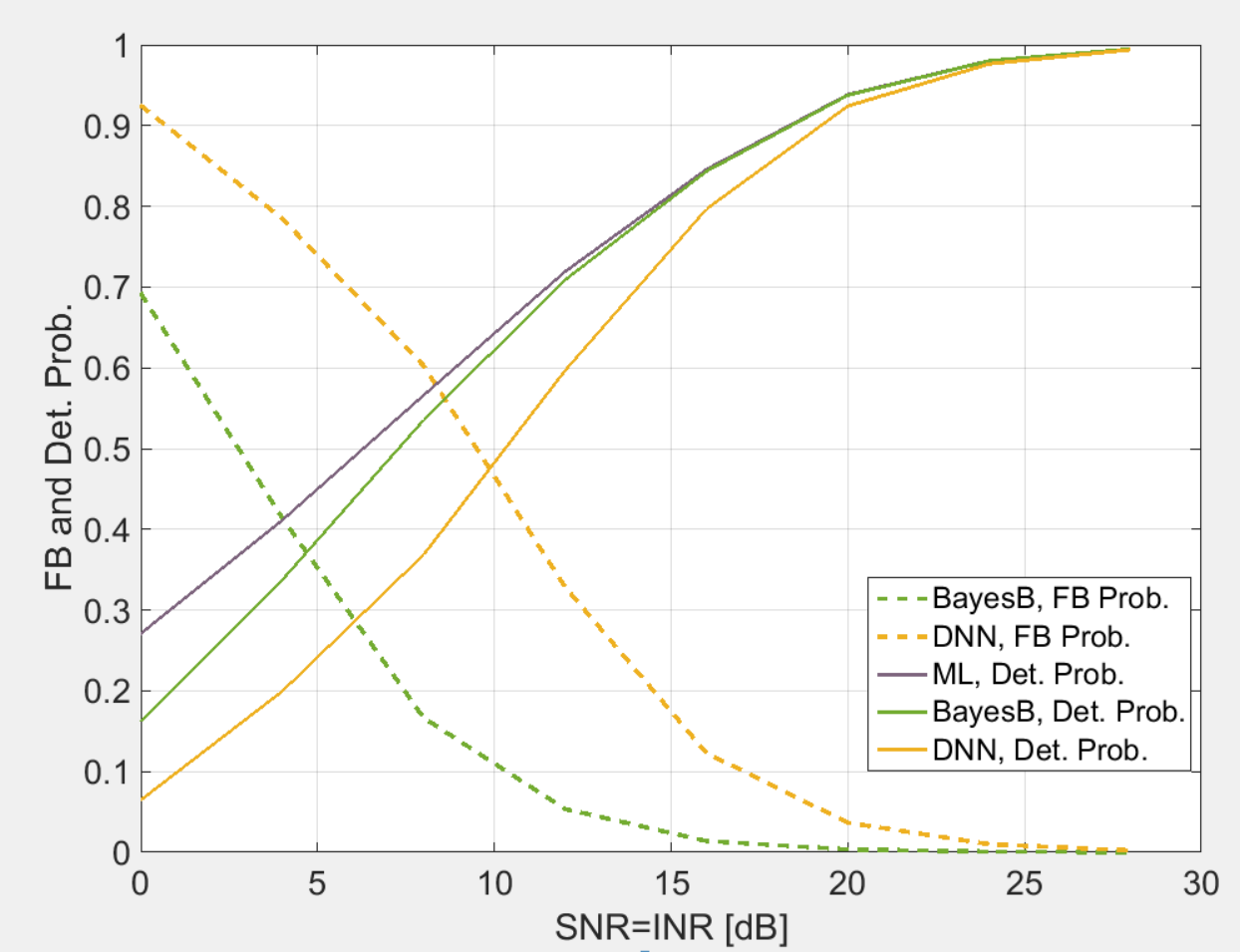
In Fig. 6, we further show the probabilities of correct MF detection and fall-back. Due to fall-back, the correct detection probabilities of Bayes-risk and DNN based fall-backs are degraded compared to the case without fall-back. But the DNN based fall-back is more aggressive in determining a fall-back than the Bayes based approach. This means that on averaged the DNN based fall-back will activate SLIC receiver much less than the other two cases, and yields a higher complexity-saving by running eIRC on more PRBs.

The detailed complexity savings by applying the fall-back mechanism depends on the types of SLIC and eIRC receivers. But we can still measure the relative complexity saving by the ratio of activating SLIC and eIRC receivers. With no fall-back, the SLIC is always running which yields the highest complexity. With Bayes-risk based fall-back, seen from Fig. 6, the fall-back probability is 10% at 10dB SNR, which only saves 10% of SLIC operations that are replaced them by eIRC. On the other hand, the fall-back probability of DNN based approach is around 50%, which replaces half SLIC operations by eIRC, and complexity savings are more significant.

Since DNN based fall-back mechanism yields a higher fall-back probability, i.e., less activation of the advanced SLIC receiver, the impact on throughput is of interest.

In Fig. 7 we test the normalized throughput on a 1.4MHz bandwidth in long-term-evolution (LTE) system [1] under the conditions that $\boldsymbol{s}$ is QPSK modulated while $\boldsymbol{x}$ uses 16QAM, and with a code-rate 0.5. The MF detection on each physical resource block (PRB) is independent and based on the first 24 samples.

As can be seen that the gains between eIRC and SLIC with genie MF is close to 4dB at 90% throughput. Surprisingly, the case without fall-back performs quite close to the ideal throughput, and so are the cases with Bayes and DNN based fall-back mechanisms. However, as the later two approaches activating less SLIC compared to the case without fall-back, the savings in complexity are still siginificant. Especially with the DNN based fall-back, the computational-cost saving is much higher than Bayes based fall-back, as seen from Fig. 6, but throughput losses compared to others is marginal.

References

- [1] 3GPP TR 36.866, Study on network-assisted interference cancellation and suppression (NAIC) for LTE, Rel. 12, Jan. 2015.
- [2] G. Morozov and A. Davydov, “Decoding-aided parameter estimation for interference cancellation and suppression receivers in LTE-advanced systems”, IEEE Veh. Techno. Conf. (VTC-Spring), Glasgow, UK, May, 2015, pp. 1-5.
- [3] D. Bai, J. Lee, S. Kim, and I. Kang, “Near ML modulation classification”, IEEE Veh. Techno. Conf. (VTC-Fall), Quebec City, Canada, Sept. 2012, pp. 1-5.
- [4] B. Kim, J. Kim, H. Chae, D. Yoon, and J. W. Choi, “Deep neural network-based automatic modulation classification technique,” Int. Conf. Inf. Commun, Techno. Conv. (ICTC), Jeju, South Korea, Oct. 2016, pp. 579-582.
- [5] X. Liu, D. Yang, and A. E. Gamal, “Deep neural network architectures for modulation classification,” Asilomar Conf. Signals, Syst. Comput. (ACSSC), Pacific Grove, CA, USA, Nov. 2017, pp. 919-915.
- [6] S. M. Kay, Fundamentals of statistical signal processing. vol. 2., detection theory, Prentice-Hall signal processing series, Upper Saddle River, NJ, USA, 1998.