跳到论文正文
W Papers独立论文阅读器 arXiv:1905.10686 论文正文 计算阅读时间 · 0%
引用这篇论文根据当前论文元数据生成,正式投稿前建议核对。


License: arXiv.org perpetual non-exclusive license
arXiv:1905.10686v2 [stat.ML] 23 Jul 2021

Empirical Risk Minimization in the Interpolating Regime with Application to Neural Network Learning

Nicole Mücke Affiliation: Institute for Mathematical Stochastics Affiliation: Technical University of Braunschweig Email: nicole.muecke@tu-braunschweig.de    Ingo Steinwart Affiliation: Institute for Stochastics and Applications Affiliation: University of Stuttgart Email: ingo.steinwart@mathematik.uni-stuttgart.de
August 11, 2026
Abstract

A common strategy to train deep neural networks (DNNs) is to use very large architectures and to train them until they (almost) achieve zero training error. Empirically observed good generalization performance on test data, even in the presence of lots of label noise, corroborate such a procedure. On the other hand, in statistical learning theory it is known that over-fitting models may lead to poor generalization properties, occurring in e.g. empirical risk minimization (ERM) over too large hypotheses classes. Inspired by this contradictory behavior, so-called interpolation methods have recently received much attention, leading to consistent and optimally learning methods for some local averaging schemes with zero training error. However, there is no theoretical analysis of interpolating ERM-like methods so far. We take a step in this direction by showing that for certain, large hypotheses classes, some interpolating ERMs enjoy very good statistical guarantees while others fail in the worst sense. Moreover, we show that the same phenomenon occurs for DNNs with zero training error and sufficiently large architectures.

1 Introduction

During the last few decades statistical learning theory (SLT) has developed powerful techniques to analyze many variants of (regularized) empirical risk minimizers (ERMs), see e.g. [8, 23, 22, 10, 19, 21, 18]. The resulting learning guarantees, which include finite sample bounds, oracle inequalities, learning rates, adaptivity, and consistency, assume in most cases that the effective hypotheses space of the considered method is sufficiently small in terms of some notion of capacity such as VC-dimension, fat-shattering dimension, Rademacher complexities, covering numbers, or eigenvalues.

Most training algorithms for DNNs also optimize an (regularized) empirical error term over a hypotheses space, namely the class of functions that can be represented by the architecture of the considered DNN, see [9, Part II]. However, unlike for many classical ERMs, the hypotheses space is parametrized in a rather complicated manner. Consequently, the optimization problem is, in general, harder to solve. A common way to address this is in practice is to use very large DNNs, since despite their size, training them is often easier, see e.g. [17, 13] and the references therein. Now, for sufficiently large DNNs it has been recently observed that common training algorithms can achieve zero training error on randomly, or arbitrarily labeled training sets, see [24]. Because of this ability, their effective hypotheses space can no longer have a sufficiently small capacity in the sense of classical SLT, so that the usual techniques for analyzing learning algorithms are no longer suitable, see e.g. the discussion on this in [24, 4, 15, 25]. In fact, SLT provides well known examples of large hypotheses spaces for which zero training error is possible but a simple ERM fails to learn. This phenomenon is known as over-fitting, and common wisdom suggests that successful learning algorithms need to avoid over-fitting, see e.g. [10, pp. 21-22]. The empirical evidence mentioned above thus stands in stark contrast to this credo of SLT.

This somewhat paradoxical behavior has recently sparked interests, leading to deeper theoretical investigations of the so called double/ multiple-descent phenomenon for different model settings. More specifically, [5] analyzed linear regression with random feature selection and investigated the random Fourier feature model. This model has also been analyzed by [14]. For linear regression, where model complexity is measured in terms of the number of parameters, the authors in [2, 20] show that over-parameterization is even essential for benign over-fitting. However, these results are highly distribution dependent and require a specific covariance structure and (sub-) Gaussian data. For more details we refer also to [4, 7, 12, 16, 1]. Another line of research [6] shows for classical learning methods, namely Nadaraya-Watson estimator with certain singular kernels, that interpolating the training data can achieve optimal rates for problems of nonparametric regression and prediction with square loss. Beyond empirical evidence there are therefore also theoretical results showing that interpolating the data and good learning performance is simultaneously possible. So far, however, the considered interpolating learning methods do not implement an empirical risk minimization (ERM) scheme nor do they closely resemble the learning mechanisms of DNNs. In this paper, we take a step towards closing this gap.

First, we explicitly construct, for data sets of size nn, large classes of hypotheses ℋn{\mathcal{H}}_{n} for which we show that some interpolating least squares ERM algorithms over ℋn{\mathcal{H}}_{n} enjoy very good statistical guarantees, while other interpolating least squares ERM algorithms over ℋn{\mathcal{H}}_{n} fail in a strong sense. To be more precise, we observe the following phenomena: There exists a universally consistent ERM and there exists an ERM whose predictors converge to the negative regression function for most distributions. In particular, the latter ERM is not consistent for most distributions, and even worse, the obtained risks are usually for off the best possible risk. We further construct modifications that enjoy minmax optimal rates of convergence up to some log factor under standard assumptions. In addition, there are also ERM algorithms that exhibit an intermediate behavior between these two extreme cases, with arbitrarily slow convergence. To put this in perspective, we note that classical SLT shows that for sufficiently small hypotheses classes, all versions of ERM enjoy good statistical guarantees. In contrast, our results demonstrate that this is no longer true for large hypotheses classes. For such hypotheses spaces, the description “ERM” is thus not sufficient to identify well-behaving learning algorithms. Instead, the class of algorithms described by “ERM” over such hypotheses spaces may encompass learning algorithms with extremely distinct learning behavior.

Second, we show that exactly the same phenomena occur for interpolating ReLU-DNNs of at least two hidden layers with widths growing linearly in both input dimension dd and sample size nn. We present DNN training algorithms that produce interpolating predictors and that enjoy consistency and optimal rates, at least up to some log factor. In addition, this training can be done in 𝒪⁡(d2⋅n2){\mathcal{O}}(d^{2}\cdot n^{2})-time if the DNNs are implemented as fully connected networks. Since the constructed predictors have a particularly sparse structure, the training time can actually be reduced to 𝒪⁡(d⋅n⋅log⁡n){\mathcal{O}}(d\cdot n\cdot\log n) by implementing the DNNs as loosely connected networks. Moreover, we show that there are other efficient and feasible training algorithms for exactly the same architectures that fail in the worst possible sense, and like in the ERM case, there are also a variety of training algorithms performing in between these two extreme cases.

The rest of the paper is organized as follows: In Section 2 we firstly recall classical histograms as ERMs that we extend then to the class of inflated histograms. We provide specific examples of interpolating predictors from that class. In our main theorems we derive consistency results and learning rates. In the following Section 3 we explain how inflated histograms can be approximated by ReLU networks, having analogous learning properties.

All our proofs are deferred to the Appendices A, B, C, and D. Finally, in the supplementary material E we derive general uniform bounds for histograms based on data-dependent partitions. This result is needed for proving our main results and is of independent interest.

2 The histogram rule revisited

In this section we reconsider the histogram rule in the framework of regression. In more detail, we recall the classical histogram rule and show how to change this appropriately in order to obtain a predictor that is able to interpolate given data. To this end, let us begin by introducing the necessary notations. Throughout this work, we consider X:=[−1,1]dX:=[-1,1]^{d} and Y=[−1,1]Y=[-1,1] if not specified otherwise. Moreover, L:Y×ℝ→[0,∞)L:Y\times\mathbb{R}\to[0,\infty) denotes the least squares loss L⁡(y,t)=(y−t)2L(y,t)=(y-t)^{2}. Given a dataset D:=((x1,y1),…,(xn,yn))∈(X×Y)nD:=((x_{1},y_{1}),...,(x_{n},y_{n}))\in(X\times Y)^{n} drawn i.i.d. from an unknown distribution PP on X×YX\times Y, the aim of supervised learning is to build a function fD:X→ℝf_{D}:X\to\mathbb{R} based on DD such that its risk

ℛL,P​(fD):=∫X×YL⁡(y,fD​(x))​𝑑P​(x,y),{{\cal R}_{L,P}(f_{D})}:=\int_{X\times Y}L(y,f_{D}(x))\;dP(x,y)\;, (1)

is close to the smallest possible risk

ℛL,P∗=inff:X→ℝℛL,P(f).{{\cal R}^{*}_{L,P}}=\inf_{f:X\to\mathbb{R}}{{\cal R}_{L,P}(f)}\,. (2)

In the following, ℛL,P∗{{\cal R}^{*}_{L,P}} is called the Bayes risk and an fL,P∗:X→ℝ{f_{L,P}^{*}}:X\to\mathbb{R} satisfying ℛL,P​(fP∗)=ℛL,P∗{{\cal R}_{L,P}(f^{*}_{P})}={{\cal R}^{*}_{L,P}} is called Bayes decision function. Recall, that for the least squares loss, fL,P∗{f_{L,P}^{*}} equals the conditional mean function, i.e. fL,P∗​(x)=𝔼P​(Y|x){f_{L,P}^{*}}(x)=\mathbb{E}_{P}(Y|x) for PXP_{X}-almost all x∈Xx\in X, where PXP_{X} denotes the marginal distribution of PP on XX. In general, estimators fDf_{D} having small excess risk

ℛL,P​(fD)−ℛL,P∗=‖fD−fL,P∗‖L2​(PX)2,{{\cal R}_{L,P}(f_{D})}-{{\cal R}^{*}_{L,P}}=||f_{D}-{f_{L,P}^{*}}||_{L_{2}(P_{X})}^{2}\;, (3)

where ∥⋅∥L2​(PX)\|\cdot\|_{L_{2}(P_{X})} denotes the usual L2L_{2}-norm with respect to PXP_{X}, are considered as good in classical statistical learning theory.

Now, to describe the class of learning algorithms we are interested in, we need the empirical risk of an f:X→ℝf:X\to\mathbb{R}, i.e.

ℛL,D​(f):=1n​∑i=1nL⁡(yi,f⁡(xi)).{{\cal R}_{L,D}(f)}:=\frac{1}{n}\sum_{i=1}^{n}L(y_{i},f(x_{i}))\;.

Recall, that an empirical risk minimizer (ERM) over some set ℱ{\cal F} of functions f:X→ℝf:X\to\mathbb{R} chooses, for every data set DD, an fD∈ℱf_{D}\in{\mathcal{F}} that satisfies

ℛL,D​(fD)=inff∈ℱℛL,D​(f).{{\cal R}_{L,D}(f_{D})}=\inf_{f\in{\mathcal{F}}}{{\cal R}_{L,D}(f)}\,.

Note that the definition of ERMs implicitly requires that the infimum on the right hand side is attained, namely by fDf_{D}. In general, however, fDf_{D} does not need to be unique. It is well-known that if we have a suitably increasing sequence of hypotheses classes ℱn{\mathcal{F}}_{n} with controlled capacity, then every ERM D↦fDD\mapsto f_{D} that ensures fD∈ℱnf_{D}\in{\mathcal{F}}_{n} for all data sets DD of length nn learns in the sense of e.g. universal consistency, and under additional assumptions it may also enjoy minmax optimal learning rates, see e.g. [8, 22, 10, 19].

2.1 Classical Histograms

Particular simple ERMs are histogram rules (HRs). To recall the latter, we fix a finite partition 𝒜=(Aj)j∈J{\cal A}=(A_{j})_{j\in J} of XX and for x∈Xx\in X we write A⁡(x)A(x) for the unique cell AjA_{j} with x∈Ajx\in A_{j}. Moreover, we define

ℋ𝒜:={∑j∈Jcj​𝟏Aj:cj∈Y},\displaystyle{\mathcal{H}}_{{\cal A}}:=\biggl\{\sum_{j\in J}c_{j}\bm{1}_{A_{j}}\;:\;c_{j}\in Y\biggr\}\;, (4)

where 𝟏Aj\bm{1}_{A_{j}} denotes the indicator function of the cell AjA_{j}. Now, given a data set DD and a loss LL an 𝒜{\cal A}-histogram is an hD,𝒜=∑j=1mcj∗​𝟏Aj∈ℋ𝒜h_{D,{\cal A}}=\sum_{j=1}^{m}c_{j}^{*}\bm{1}_{A_{j}}\in{\mathcal{H}}_{{\cal A}} that satisfies

∑i:xi∈AjL(xi,yi,cj∗)=infc∈Y∑i:xi∈AjL(xi,yi,c)\displaystyle\sum_{i:x_{i}\in A_{j}}L(x_{i},y_{i},c^{*}_{j})=\inf_{c\in Y}\sum_{i:x_{i}\in A_{j}}L(x_{i},y_{i},c) (5)

for all, so-called non-empty cells AjA_{j}, that is, cells AjA_{j} with Nj:=|{i:xi∈Aj}|>0N_{j}:=|\{i:x_{i}\in A_{j}\}|>0. Clearly, D↦hD,𝒜D\mapsto h_{D,{\cal A}} is an ERM. Moreover, note that in general hD,𝒜h_{D,{\cal A}} is not uniquely determined, since cj∗∈Yc_{j}^{*}\in Y can take arbitrary values for empty cells AjA_{j}. In particular, there are more than one ERM over ℋ𝒜{\mathcal{H}}_{{\cal A}} as soon as m,n≥2m,n\geq 2.

Before we proceed, let us consider the specific example of the least squares loss in more detail. Here, a simple calculation shows, see Lemma A.1, that for all non-empty cells AjA_{j}, the coefficient cj∗c_{j}^{*} in (5) is uniquely determined by

cj∗:=1Nj∑i:xi∈Ajyic_{j}^{*}:=\frac{1}{N_{j}}\sum_{i:x_{i}\in A_{j}}y_{i}\; (6)

provided that YY is convex. In the following, we call every resulting D↦hD,𝒜D\mapsto h_{D,{\cal A}} with

hD,𝒜:=∑j=1mcj∗​𝟏Aj∈ℋ𝒜h_{D,{\cal A}}:=\sum_{j=1}^{m}c_{j}^{*}\bm{1}_{A_{j}}\in{\mathcal{H}}_{{\cal A}}

an empirical HR for regression with respect to the least-squares loss LL. For later use we also introduce an infinite sample version of a classical histogram

hP,𝒜:=∑j∈Jcj∗​𝟏Aj, where cj∗:=1PX​(Aj)​∫AjfL,P∗​(x)​d​PX​(x)h_{P,{\mathcal{A}}}:=\sum_{j\in J}c^{*}_{j}\bm{1}_{A_{j}}\;,\qquad\qquad\mbox{ where }\quad c^{*}_{j}:=\frac{1}{P_{X}(A_{j})}\int_{A_{j}}{f_{L,P}^{*}}(x)dP_{X}(x)\; (7)

for all cells AjA_{j} with PX​(Aj)>0P_{X}(A_{j})>0. Similarly to empirical histograms one has

ℛL,P​(hP,𝒜)=infh∈ℋ𝒜ℛL,P​(h).{\mathcal{R}}_{L,P}(h_{P,{\mathcal{A}}})=\inf_{h\in{\mathcal{H}}_{\mathcal{A}}}{\mathcal{R}}_{L,P}(h)\;.

We are mostly interested in HRs on X=[−1,1]dX=[-1,1]^{d} whose underlying partition essentially consists of cubes with a fixed width. To rigorously deal with boundary effects, we first say that a partition (Bj)j≥1(B_{j})_{j\geq 1} of ℝd\mathbb{R}^{d} is a cubic partition of width s>0s>0, if each cell BjB_{j} is a translated version of [0,s)d[0,s)^{d}, i.e. there is an x†∈ℝdx^{\dagger}\in\mathbb{R}^{d} called offset such that for all j≥1j\geq 1 there exist kj:=(k1,…,kd)∈ℤdk_{j}:=(k_{1},\dots,k_{d})\in\mathbb{Z}^{d} with

Bj=x†+skj+[0,s)d.\displaystyle B_{j}=x^{\dagger}+sk_{j}+[0,s)^{d}\,. (8)

Now, a partition 𝒜=(Aj)j∈J{\cal A}=(A_{j})_{j\in J} of X=[−1,1]dX=[-1,1]^{d} is called a cubic partition of width s>0s>0, if there is a cubic partition ℬ=(Bj)j≥1{\mathcal{B}}=(B_{j})_{j\geq 1} of ℝd\mathbb{R}^{d} with width s>0s>0 such that J={j≥1:Bj∩X≠∅}J=\{j\geq 1:B_{j}\cap X\neq\emptyset\} and Aj=Bj∩XA_{j}=B_{j}\cap X for all j∈Jj\in J. If s∈(0,1]s\in(0,1], then, up to reordering, this (Bj)j≥1(B_{j})_{j\geq 1} is uniquely determined by 𝒜{\cal A}.

If the hypotheses space (4) is based on a cubic partition of X=[−1,1]dX=[-1,1]^{d} with width s>0s>0, then the resulting HRs are well understood. For example, universal consistency and learning rates have been established, see e.g. [8, 10]. In general, these results only require a suitable choice for the widths s=sns=s_{n} for n→∞n\to\infty but no specific choice of the cubic partition of width ss. For this reason we write ℋs:=⋃ℋ𝒜{\cal H}_{s}:=\bigcup{\cal H}_{{\cal A}}, where the union runs over all cubic partitions 𝒜{\cal A} of XX with fixed width s∈(0,1]s\in(0,1].

2.2 Interpolating Predictors and Inflated Histograms

In this section we construct particular interpolating ERMs. In a nutshell, the basic idea is to first consider classical histogram rules, and then to inflate their hypotheses space so that we can find interpolating ERMs in these inflated hypotheses spaces.

Definition 2.1 (Interpolating Predictor).

We say that an f:X→Yf:X\to Y interpolates DD, if

ℛL,D(f)=ℛL,D∗:=inff~:X→ℝℛL,D(f~),{{\cal R}_{L,D}(f)}={{\cal R}^{*}_{L,D}}:=\inf_{\tilde{f}:X\to\mathbb{R}}{{\cal R}_{L,D}(\tilde{f})}\,,

where we emphasize that the infimum is taken over all ℝ\mathbb{R}-valued functions, while ff is required to be YY-valued.

Clearly, an f:X→Yf:X\to Y interpolates DD if and only if

∑k:xk=xi∗L(xi,yi,f(xi∗))=infc∈ℝ∑k:xk=xi∗L(xi,yi,c),i=1,…,m,\displaystyle\sum_{k:x_{k}=x_{i}^{*}}L(x_{i},y_{i},f(x_{i}^{*}))=\inf_{c\in\mathbb{R}}\sum_{k:x_{k}=x_{i}^{*}}L(x_{i},y_{i},c)\,,\qquad\qquad i=1,\dots,m, (9)

where x1∗,…,xm∗x_{1}^{*},\dots,x_{m}^{*} are the elements of DX:={xi:i=1,…,n}D_{X}:=\{x_{i}:i=1,\dots,n\}.

It is easy to check that for the least squares loss LL and all data sets DD there exists an fD∗f_{D}^{*} interpolating DD. Moreover, we have ℛL,D∗>0{{\cal R}^{*}_{L,D}}>0 if and only if DD contains contradicting samples, i.e. xi=xkx_{i}=x_{k} but yi≠yky_{i}\neq y_{k}. Finally, if ℛL,D∗=0{{\cal R}^{*}_{L,D}}=0, then any interpolating fD∗f_{D}^{*} needs to satisfy fD∗​(xi)=yif_{D}^{*}(x_{i})=y_{i} for all i=1,…,ni=1,\dots,n.

Definition 2.2 (Interpolatable Loss).

We say that LL is interpolatable for DD if there exists an f:X→Yf:X\to Y that interpolates DD, i.e. ℛL,D​(f)=ℛL,D∗{{\cal R}_{L,D}(f)}={{\cal R}^{*}_{L,D}}.

Note that (9) in particular ensures that the infimum over ℝ\mathbb{R} on the right is attained at some ci∗∈Yc^{*}_{i}\in Y. Many common losses including the least squares, the hinge, and the classification loss interpolate all DD, and for the latter three losses we have ℛL,D∗>0{{\cal R}^{*}_{L,D}}>0 if and only if DD contains contradicting samples, i.e. xi=xkx_{i}=x_{k} but yi≠yky_{i}\neq y_{k}. Moreover, for the least squares loss, ci∗c^{*}_{i} can be easily computed by averaging over all labels yky_{k} that belong to some sample xkx_{k} with xk=xix_{k}=x_{i}.

Let us now describe more precisely the inflated versions of ℋs{\cal H}_{s}. For r,s>0r,s>0 and m≥0m\geq 0 we want to consider functions

f=h+∑i=1mbi​𝟏xi∗+t​B∞f=h+\sum_{i=1}^{m}b_{i}\bm{1}_{x_{i}^{*}+tB_{\infty}} (10)

with h∈ℋs,bi∈2​Y,xi∗∈X,h\in{\cal H}_{s},\,b_{i}\in 2Y,\,x_{i}^{*}\in X, and t∈[0,r]t\in[0,r], where B∞:=[−1,1]dB_{\infty}:=[-1,1]^{d}. In other words, for m≥1m\geq 1, such an ff changes a classical histogram h∈ℋsh\in{\cal H}_{s} on at most mm small neighborhoods of some arbitrary points x1∗,…,xm∗x_{1}^{*},\dots,x_{m}^{*} in XX. Such changes are useful for finding interpolating predictors. In general, these small neighborhoods xi∗+t​B∞x_{i}^{*}+tB_{\infty} however may intersect and may be contained in more than one cell AjA_{j} of the considered partition 𝒜{\cal A} with h∈ℋ𝒜h\in{\mathcal{H}}_{\mathcal{A}}. To avoid undesired boundary effects we restrict the class of all admissible cubic partitions 𝒜{\mathcal{A}} of XX associated with hh. An additional technical difficulty arises in particular when constructing interpolating predictors since the set of points {x1∗,…,xm∗}⊂X\{x_{1}^{*},...,x_{m}^{*}\}\subset X are naturally the random input variables. As a consequence, the admissible cubic partitions become data-dependent. As a next step, we introduce the notion of a partitioning rule. To this end, we write

Potm​(X):={A⊂X:|A|=m}\displaystyle\mathrm{Pot}_{m}(X):=\bigl\{A\subset X:|A|=m\bigr\}

for the set of all subsets of XX having cardinality mm. Moreover, we denote the set of all finite partitions of XX by 𝒫⁡(X){\mathcal{P}}(X).

Definition 2.3.

Given an integer m≥1m\geq 1, an mm-sample partitioning rule for XX is a map πm:Potm​(X)→𝒫⁡(X)\pi_{m}:\mathrm{Pot}_{m}(X)\to{\mathcal{P}}(X), i.e. a map that associates to every subset {x1∗,…,xm∗}⊂X\{x_{1}^{*},...,x_{m}^{*}\}\subset X of cardinality mm a finite partition 𝒜{\cal A}. Additionally, we will call an mm-sample partitioning rule that assigns to any such {x1∗,…,xm∗}∈Potm​(X)\{x_{1}^{*},...,x_{m}^{*}\}\in\mathrm{Pot}_{m}(X) a cubic partition with fixed width s∈(0,1]s\in(0,1] an mm-sample cubic partitioning rule and write πm,s\pi_{m,s}.

Next we explain in more detail which particular partitions are considered as admissible.

Definition 2.4 (Proper Alignment).

Let 𝒜{\mathcal{A}} be a cubic partition of XX with width s∈(0,1]s\in(0,1], ℬ{\mathcal{B}} be the partition of ℝd\mathbb{R}^{d} that defines 𝒜{\cal A}, and r∈(0,s)r\in(0,s). We say that 𝒜{\mathcal{A}} is properly aligned to the set of points {x1∗,…,xm∗}∈Potm​(X)\{x_{1}^{*},...,x_{m}^{*}\}\in\mathrm{Pot}_{m}(X) with parameter rr, if for all i,k=1,…,mi,k=1,\dots,m we have

xi∗+r​B∞\displaystyle x_{i}^{*}+rB_{\infty} ⊂B⁡(xi∗),\displaystyle\subset B(x_{i}^{*})\,, (11)
xi∗+r​B∞∩xk∗+r​B∞\displaystyle x_{i}^{*}+rB_{\infty}\cap x_{k}^{*}+rB_{\infty} =∅ whenever i≠k,\displaystyle=\emptyset\qquad\qquad\mbox{ whenever $i\neq k$,} (12)

where B⁡(xi∗)B(x_{i}^{*}) is the unique cell 11 1 Note that this gives A⁡(xi∗)=B⁡(xi∗)∩XA(x_{i}^{*})=B(x_{i}^{*})\cap X. of ℬ{\mathcal{B}} that contains xi∗x_{i}^{*}.

Clearly, if 𝒜{\mathcal{A}} is properly aligned with parameter r>0r>0, then it is also properly aligned for any parameter t∈[0,r]t\in[0,r] for the same set of points {xj∗}j=1m\{x_{j}^{*}\}_{j=1}^{m} in Potm​(X)\mathrm{Pot}_{m}(X). Moreover, any cubic partition 𝒜{\mathcal{A}} of XX with width s>0s>0 is properly aligned with the parameter r=0r=0 for any set of points {xj∗}j=1m\{x_{j}^{*}\}_{j=1}^{m} in Potm​(X)\mathrm{Pot}_{m}(X).

In what follows, we establish the existence of cubic partitions 𝒜{\mathcal{A}} that are properly aligned to a given set of points with parameter r>0r>0 being sufficiently small. In other words, we construct a special mm-sample cubic partitioning rule πm,s\pi_{m,s}. We call henceforth any such rule πm,s\pi_{m,s} an mm-sample properly aligned cubic partitioning rule. To this end, let DX:={x1∗,…,xm∗}∈Potm​(X)D_{X}:=\{x_{1}^{*},...,x_{m}^{*}\}\in\mathrm{Pot}_{m}(X) be a set points and note that (12) holds for all r>0r>0 satisfying

r<12mini,k:i≠k∥xi∗−xk∗∥∞.r<\frac{1}{2}\min_{i,k:i\neq k}\|x_{i}^{*}-x_{k}^{*}\|_{\infty}\;.

Clearly, a brute-force algorithm finds such an rr in 𝒪⁡(d​m2){\cal O}(dm^{2})-time. However, a smarter approach is to first sort the first coordinates x1,1∗,…,xm,1∗x_{1,1}^{*},\dots,x_{m,1}^{*} and to determine the smallest positive distance r1r_{1} of two consecutive, non-identical ordered coordinates. This approach is then repeated for the remaining d−1d-1-coordinates, so at the end we have r1,…,rd>0r_{1},\dots,r_{d}>0. Then

r∗:=rDX∗:=13​min⁡{r1,…,rd}r^{*}:=r^{*}_{D_{X}}:=\frac{1}{3}\min\{r_{1},\dots,r_{d}\} (13)

satisfies (12) and the used algorithm is 𝒪⁡(d⋅m​log⁡m){\cal O}(d\cdot m\log m) in time. Our next result shows that we can also ensure (11) by jiggling the cubic partitions. Being rather technical, the proof is deferred to the Appendix B.

Theorem 2.5 (Existence of Properly Aligned Cubic Partitioning Rule).

For all d≥1d\geq 1, s∈(0,1]s\in(0,1], and m≥1m\geq 1 there exist an mm-sample cubic partitioning rule πm,s\pi_{m,s} with |Im⁡(πm,s)|≤(m+1)d|\Image(\pi_{m,s})|\leq(m+1)^{d} that assigns to each set of points DX:={x1∗,…,xm∗}∈Potm​(X)D_{X}:=\{x_{1}^{*},...,x_{m}^{*}\}\in\mathrm{Pot}_{m}(X) a cubic partition 𝒜{\cal A} that is properly aligned to {x1∗,…,xm∗}\{x_{1}^{*},...,x_{m}^{*}\} with parameter r:=rDX:=min⁡{r∗,s3​m+3}r:=r_{D_{X}}:=\min\{r^{*},\frac{s}{3m+3}\}, where r∗=rDX∗r^{*}=r^{*}_{D_{X}} is defined in (13).

The construction of an mm-sample cubic partitioning rule πm,s\pi_{m,s} basically relies on the representation (8) of cubic partitions ℬ{\mathcal{B}} of ℝd\mathbb{R}^{d}. In fact, the proof of Theorem 2.5 shows that there exists a finite set x1†,…,xK†∈ℝdx_{1}^{\dagger},...,x^{\dagger}_{K}\in\mathbb{R}^{d} of candidate offsets, with K=(m+1)dK=(m+1)^{d}. While at first glance this number seems to be prohibitively large for an efficient search, it turns out that the proof of Theorem (2.5) actually provides a simple algorithm that is 𝒪⁡(d⋅m){\cal O}(d\cdot m) in time for identifying coordinate-wise the xℓ†x_{\ell}^{\dagger} that leads to πm,s​({x1∗,…,xm∗})\pi_{m,s}(\{x_{1}^{*},...,x_{m}^{*}\}) .

Being now well prepared, we introduce the class of inflated histograms.

Definition 2.6.

Let s∈(0,1]s\in(0,1] and m≥1m\geq 1. Then a function f:X→Yf:X\to Y is called an mm-inflated histogram of width ss, if there exist a subset {x1∗,…,xm∗}∈Potm​(X)\{x_{1}^{*},...,x_{m}^{*}\}\in\mathrm{Pot}_{m}(X) and a cubic partition 𝒜{\cal A} of width ss that is properly aligned to {x1∗,…,xm∗}\{x_{1}^{*},...,x_{m}^{*}\} with parameter r∈[0,s)r\in[0,s) such that

f=h+∑i=1mbi​𝟏xi∗+t​B∞,\displaystyle f=h+\sum_{i=1}^{m}b_{i}\bm{1}_{x_{i}^{*}+tB_{\infty}}\,,

where h∈ℋ𝒜h\in{\mathcal{H}}_{\mathcal{A}}, t∈[0,r]t\in[0,r], and bi∈2​Yb_{i}\in 2Y for all i=1,…,mi=1,\dots,m. We denote the set of all mm-inflated histograms of width ss by ℱs,m{\mathcal{F}}_{s,m}. Moreover, for n≥1n\geq 1 we write

ℱs,n∗:=ℱs,1∪⋯∪ℱs,n.\displaystyle{\cal F}^{*}_{s,n}:={\cal F}_{s,1}\cup\dots\cup{\cal F}_{s,n}\,.

Note that the condition t≤r<st\leq r<s ensures that the representation f=h+∑i=1mbi​𝟏xi∗+t​B∞f=h+\sum_{i=1}^{m}b_{i}\bm{1}_{x_{i}^{*}+tB_{\infty}} of any f∈ℱs,mf\in{\mathcal{F}}_{s,m} is unique.In addition, given an f∈ℱs,n∗f\in{\cal F}^{*}_{s,n}, the number mm of inflation points {x1∗,…,xm∗}\{x_{1}^{*},...,x_{m}^{*}\} is uniquely determined, too, and hence so is the representation of ff.

Refer to caption
Refer to caption
Figure 1: Left. Depiction of an inflated histogram for regression for a cubic partition 𝒜=(Aj)j∈J{\mathcal{A}}=(A_{j})_{j\in J} that is not properly aligned to the data (black crosses). The predictions ci∗c_{i}^{*} and cj∗c_{j}^{*} on the associated cells AiA_{i} and AjA_{j} are calculated according to (6), i.e. by a local average. Mispredicted samples are corrected according to (14) on a t​B∞tB_{\infty}-neighborhood for some small t>0t>0. Note that one sample is too close to the cell boundary, i.e. (11) is violated. Right. An inflated histogram that is properly aligned to the same data set. Note that (11) ensures that boundary effects as for the left HR do not take place. For inflated histograms these effects seem to be a negligible technical nuisance. For their DNN counterparts considered in Section 3, however, such effects may significantly complicate the constructions of interpolating predictors, see Figure 2.

So far we have formalized the notion of interpolation and defined an appropriate inflated hypotheses class for modified histograms. In our next result we go a step further by providing a sufficient condition for the existence of interpolating predictors in ℱs,m{\mathcal{F}}_{s,m}.

Proposition 2.7.

Let LL be a loss that is interpolatable for D=((x1,yi),…,(xn,yn))D=((x_{1},y_{i}),\dots,(x_{n},y_{n})) and let x1∗,…,xm∗x_{1}^{*},\dots,x_{m}^{*} be as in (9). Moreover, for s∈(0,1]s\in(0,1] and r>0r>0 we fix an f∗∈ℱs,mf^{*}\in{\mathcal{F}}_{s,m} with representation as given in Definition 2.6. For i=1,…,mi=1,\dots,m let jij_{i} be the index such that xi∗∈Ajix_{i}^{*}\in A_{j_{i}}. Then f∗f^{*} interpolates DD, if for all i=1,…,mi=1,\dots,m we have

bi=−cji+argminc∈Y∑k:xk=xi∗L(xk,yk,c).\displaystyle b_{i}=-c_{j_{i}}+\arg\min_{c\in Y}\sum_{k:x_{k}=x_{i}^{*}}L(x_{k},y_{k},c)\,. (14)

Proof of Proposition 2.7: By our assumptions we have

ci∗:=bi+cji∈argminc∈Y∑k:xk=xi∗L(xk,yk,c)=argminc∈ℝ∑k:xk=xi∗L(xk,yk,c),c_{i}^{*}:=b_{i}+c_{j_{i}}\in\arg\min_{c\in Y}\sum_{k:x_{k}=x_{i}^{*}}L(x_{k},y_{k},c)=\arg\min_{c\in\mathbb{R}}\sum_{k:x_{k}=x_{i}^{*}}L(x_{k},y_{k},c)\,,

where the last equality is a consequence of the fact that there is an f:X→Yf:X\to Y satisfying (9). Moreover, since (11) and (12) hold, we find f∗​(xi∗)=h⁡(xi∗)+bi=cji+bi=ci∗f^{*}(x_{i}^{*})=h(x_{i}^{*})+b_{i}=c_{j_{i}}+b_{i}=c_{i}^{*}, and therefore f∗f^{*} interpolates DD by (9). ∎

Note that for all cji∈Yc_{j_{i}}\in Y the value bib_{i} given by (14) satisfies bi∈2​Yb_{i}\in 2Y and we have bi=0b_{i}=0 if cjic_{j_{i}} is contained in the arg⁡min\arg\min in (14). Consequently, defining bib_{i} by (14) always gives an interpolating f∗∈ℱs,mf^{*}\in{\mathcal{F}}_{s,m}. Moreover, (14) shows that an interpolating f∗∈ℱs,mf^{*}\in{\mathcal{F}}_{s,m} can have an arbitrary histogram part h∈ℋ𝒜h\in{\cal H}_{{\cal A}}, that is, the behavior of f∗f^{*} outside the small t​B∞tB_{\infty}-neighborhoods around the samples of DD can be arbitrary. In other words, as soon as we have found a properly aligned cubic partition 𝒜{\cal A} in the sense of ℱs,m{\mathcal{F}}_{s,m}, we can pick an arbitrary histogram h∈ℋ𝒜h\in{\cal H}_{{\cal A}} and compute the bib_{i}’s by (14). Intuitively, if the chosen t​B∞tB_{\infty}-neighborhoods are sufficiently small, then the prediction capabilities of the resulting interpolating predictor are (mostly) determined by the chosen histogram part h∈ℋ𝒜h\in{\cal H}_{{\cal A}}. Based on this observation, we can now construct different, interpolating fD∗∈ℱs,mf^{*}_{D}\in{\mathcal{F}}_{s,m} that have particularly good and bad learning behaviors.

Example 2.8 (Good interpolating histogram rule).

Let LL be the least squares loss, s∈(0,1]s\in(0,1] be a cell width, ρ≥0\rho\geq 0 be an inflation parameter, and D=((x1,yi),…,(xn,yn))D=((x_{1},y_{i}),\dots,(x_{n},y_{n})) be a data set. By DX={x1∗,…,xm∗}D_{X}=\{x_{1}^{*},...,x_{m}^{*}\} we denote the set of all covariates xj∈Xx_{j}\in X with (xj,yj)(x_{j},y_{j}) belonging to the data set. For m=|DX|m=|D_{X}|, Theorem 2.5 ensures the existence of a cubic partition 𝒜D=πm,s​(DX){\mathcal{A}}_{D}=\pi_{m,s}(D_{X}) with width s∈(0,1]s\in(0,1], being properly aligned to DXD_{X} with the data-dependent parameter rr. Based on this data-dependent cubic partition 𝒜D{\mathcal{A}}_{D} we fix an empirical histogram for regression

hD,𝒜D+:=∑j∈Jcj+​𝟏Aj∈ℋsh_{D,{\cal A}_{D}}^{+}:=\sum_{j\in J}c_{j}^{+}\bm{1}_{A_{j}}\in{\cal H}_{s} (15)

with coefficients (cj+)j∈J(c_{j}^{+})_{j\in J} precisely given in (6). Applying now Proposition 2.7 gives us an fD,s,ρ+∈ℱs,m⊂ℱs,n∗f_{D,s,\rho}^{+}\in{\mathcal{F}}_{s,m}\subset{\cal F}^{*}_{s,n}, which interpolates DD and has the representation

fD,s,ρ+:=hD,𝒜D++∑i=1mbi+​𝟏xi∗+t​B∞,f_{D,s,\rho}^{+}:=h_{D,{\cal A}_{D}}^{+}+\sum_{i=1}^{m}b^{+}_{i}\bm{1}_{x_{i}^{*}+tB_{\infty}}\;,

where the b1+,…,bm+b^{+}_{1},\dots,b_{m}^{+} are calculated according to the rule (14), and t:=min⁡{r,ρ}t:=\min\{r,\rho\} is again data-dependent. We call the map D↦fD,s,ρ+D\mapsto f_{D,s,\rho}^{+} a good interpolating histogram rule.

Example 2.9 (Bad interpolating histogram rule).

Let LL be the least squares loss, s∈(0,1]s\in(0,1] be a cell width, ρ≥0\rho\geq 0 be an inflation parameter, and D=((x1,yi),…,(xn,yn))D=((x_{1},y_{i}),\dots,(x_{n},y_{n})) be a data set. Consider again a cubic partition 𝒜D=πm,s​(DX){\mathcal{A}}_{D}=\pi_{m,s}(D_{X}) with width s∈(0,1]s\in(0,1], that is properly aligned to DXD_{X} with parameter rr and fix an empirical histogram hD,𝒜D+∈ℋsh_{D,{\cal A}_{D}}^{+}\in{\cal H}_{s} as in (15). Setting t:=min⁡{r,ρ}t:=\min\{r,\rho\}, we define a predictor fD,s,ρ−∈ℱs,mf_{D,s,\rho}^{-}\in{\mathcal{F}}_{s,m} by

fD,s,ρ−:=hD,𝒜D−+∑i=1mbi−​𝟏xi∗+t​B∞,f_{D,s,\rho}^{-}:=h_{D,{\cal A}_{D}}^{-}+\sum_{i=1}^{m}b^{-}_{i}\bm{1}_{x_{i}^{*}+tB_{\infty}}\;,

with ℋ𝒜{\cal H}_{{\cal A}}-part hD,𝒜D−:=−hD,𝒜D+h_{D,{\cal A}_{D}}^{-}:=-h_{D,{\cal A}_{D}}^{+}. The b1−,…,bm−b^{-}_{1},\dots,b_{m}^{-} are calculated according to (14) and satisfy

bi−=bi++2​cji+,b_{i}^{-}=b_{i}^{+}+2c_{j_{i}}^{+}\;,

for any i=1,…,mi=1,...,m and where jij_{i} denotes the index such that xi∗∈Ajix_{i}^{*}\in A_{j_{i}}. By writing

DX+t:=⋃i=1m(xi∗+t​B∞)\displaystyle D_{X}^{+t}:=\bigcup_{i=1}^{m}\bigl(x_{i}^{*}+tB_{\infty}\bigr) (16)

we easily see that the definition of fD,s,ρ−f_{D,s,\rho}^{-} gives fD,s,ρ−∈ℱs,m⊂ℱs,n∗f_{D,s,\rho}^{-}\in{\mathcal{F}}_{s,m}\subset{\cal F}^{*}_{s,n} and

fD,s,ρ−​(x)={fD,s,ρ+​(x) if ​x∈DX+t−fD,s,ρ+​(x) if ​x∉DX+t,\displaystyle f_{D,s,\rho}^{-}(x)=\begin{cases}f_{D,s,\rho}^{+}(x)&\mbox{ if }x\in D_{X}^{+t}\\ -f_{D,s,\rho}^{+}(x)&\mbox{ if }x\not\in D_{X}^{+t}\,,\end{cases} (17)

while Proposition 2.7 ensures that fD,s,ρ−f_{D,s,\rho}^{-} interpolates DD. We call the map D↦fD,s,ρ−D\mapsto f_{D,s,\rho}^{-} a bad interpolating histogram rule and remark that tt is, like for good interpolating histogram rules, data-dependent.

Our main results below show that the description good/ bad interpolating histogram rule from the above Examples 2.8/ 2.9, respectively, is indeed justified, provided the inflation parameter is chosen appropriately. Here we recall that good learning algorithms can be described by a small excess risk, or equivalently, a small distance to the Bayes decision function fL,P∗{f_{L,P}^{*}}, see (3). To describe bad learning behavior, we denote the point spectrum of PXP_{X} by

Δ:={x∈X:PX​({x})>0},\Delta:=\{x\in X\;:\;P_{X}(\{x\})>0\}\;, (18)

see [11]. One easily verifies that Δ\Delta is at most countable, since PXP_{X} is finite. Moreover, for an arbitrary but fixed version fL,P∗{f_{L,P}^{*}} of the Bayes decision function, we write

fL,P†:=𝟏Δ​fL,P∗−𝟏X∖Δ​fL,P∗ and ℛL,P†\displaystyle{f_{L,P}^{\dagger}}:=\bm{1}_{\Delta}{f_{L,P}^{*}}-\bm{1}_{X\setminus\Delta}{f_{L,P}^{*}}\qquad\mbox{ and }\qquad{\mathcal{R}}^{\dagger}_{L,P} :=ℛL,P​(fL,P†),\displaystyle:={{\cal R}_{L,P}({f_{L,P}^{\dagger}})}\,,

where we note that ℛL,P†{\mathcal{R}}^{\dagger}_{L,P} does, of course, not depend on the choice of fL,P∗{f_{L,P}^{*}}. Moreover, note that for x∈Δx\in\Delta the value fL,P∗​(x){f_{L,P}^{*}}(x) is also independent of the choice of fL,P∗{f_{L,P}^{*}} and it holds fL,P†​(x)=fL,P∗​(x)f^{\dagger}_{L,P}(x)={f_{L,P}^{*}}(x). In contrast, for x∈X∖Δx\in X\setminus\Delta with fL,P∗​(x)≠0{f_{L,P}^{*}}(x)\neq 0 we have fL,P†​(x)≠fL,P∗​(x)f^{\dagger}_{L,P}(x)\neq{f_{L,P}^{*}}(x). In fact, a quick calculation using (3) shows

ℛL,P†−ℛL,P∗=‖fL,P†−fL,P∗‖L2​(PX)2=4​‖𝟏X∖Δ​fL,P∗‖L2​(PX)2,\displaystyle{\mathcal{R}}^{\dagger}_{L,P}-{{\cal R}_{L,P}^{*}}=\|{f_{L,P}^{\dagger}}-{f_{L,P}^{*}}\|_{{L_{2}(P_{X})}}^{2}=4\|\bm{1}_{X\setminus\Delta}{f_{L,P}^{*}}\|_{{L_{2}(P_{X})}}^{2}\,, (19)

and consequently we have ℛL,P†−ℛL,P∗>0{\mathcal{R}}^{\dagger}_{L,P}-{{\cal R}_{L,P}^{*}}>0 whenever PX​(Δ)<1P_{X}(\Delta)<1 and fL,P∗{f_{L,P}^{*}} does not almost surely vanish on X∖ΔX\setminus\Delta. It seems fair to say that the overwhelming majority of “interesting” PP fall into this category. Finally, note that in general we do not have an equality of the form (3), when we replace ℛL,P∗{{\cal R}_{L,P}^{*}} and fL,P∗{f_{L,P}^{*}} by ℛL,P†{\mathcal{R}}^{\dagger}_{L,P} and fL,P†{f_{L,P}^{\dagger}}. However, for y,t,t′∈Y=[−1,1]y,t,t^{\prime}\in Y=[-1,1] we have |L⁡(y,t)−L⁡(y,t′)|≤4​|t−t′||L(y,t)-L(y,t^{\prime})|\leq 4|t-t^{\prime}|, and consequently we find

|ℛL,P​(f)−ℛL,P†|≤4​‖f−fL,P†‖L2​(PX)\displaystyle\bigl|{{\cal R}_{L,P}(f)}-{\mathcal{R}}^{\dagger}_{L,P}\bigr|\leq 4\,\|f-{f_{L,P}^{\dagger}}\|_{{L_{2}(P_{X})}} (20)

for all f:X→Yf:X\to Y. For this reason, we will investigate the bad interpolating histogram rule only with respect to its L2L_{2}-distance to fL,P†{f_{L,P}^{\dagger}}.

Before the state our main result of this section we need to introduce one more assumption that will be required for parts of our results.

Assumption 2.10.

There exists a non-decreasing continuous map φ:ℝ+→ℝ+\varphi:\mathbb{R}_{+}\to\mathbb{R}_{+} with φ⁡(0)=0\varphi(0)=0 such that for any t≥0t\geq 0 and x∈Xx\in X one has PX​(x+t​B∞)≤φ⁡(t)P_{X}(x+tB_{\infty})\leq\varphi(t).

Note that this assumption implies PX​({x})=0P_{X}(\{x\})=0 for any x∈Xx\in X. Moreover, it is satisfied for the uniform distribution PXP_{X}, if we consider ϕ⁡(t):=2d​td\phi(t):=2^{d}t^{d}, and a simple argument shows that modulo the constant appearing in ϕ\phi the same is true if PXP_{X} only has a bounded Lebesgue density. The latter is, however, not necessary. Indeed, for X=[−1,1]X=[-1,1] and 0<β<10<\beta<1 it is easy to construct unbounded Lebesgue densities that satisfy Assumption 2.10 for ϕ\phi of the form ϕ⁡(t)=c​tβ\phi(t)=ct^{\beta}, and higher dimensional analogons are also easy to construct. Moreover, in higher dimensions Assumption 2.10 also applies to various distributions living on sufficiently smooth low-dimensional manifolds.

With these preparations we can now establish the following theorem that shows that for ρ=0\rho=0 the good interpolating histogram rule is universally consistent while the bad interpolating histogram rule fails to be consistent in a stark sense. It further shows consistency, respectively non-consistency for ρ=ρn>0\rho=\rho_{n}>0 with ρn→0\rho_{n}\to 0.

Theorem 2.11.

Let LL be the least-squares loss and let D∈(X×Y)nD\in(X\times Y)^{n} be an i.i.d. sample of size n≥1n\geq 1. Let D↦fD,s,ρ+D\mapsto f_{D,s,\rho}^{+} denote the good interpolating histogram rule from Example 2.8. Similarly, let D↦fD,s,ρ−D\mapsto f_{D,s,\rho}^{-} denote the bad interpolating histogram rule from Example 2.9. Assume that (sn)n∈ℕ(s_{n})_{n\in\mathbb{N}} is a sequence with sn→0s_{n}\rightarrow 0 as well as ln⁡(n​snd)n​snd→0\frac{\ln(ns_{n}^{d})}{ns_{n}^{d}}\to 0 as n→∞n\to\infty.

  1. i)

    (Non)-consistency for ρn=0\rho_{n}=0. We have in probability for |D|→∞|D|\to\infty

    ‖fD,sn,0+−fL,P∗‖L2​(PX)\displaystyle\|f_{D,s_{n},0}^{+}-{f_{L,P}^{*}}\|_{{L_{2}(P_{X})}} →0,\displaystyle\to 0\,, (21)
    ‖fD,sn,0−−fL,P†‖L2​(PX)\displaystyle\|f_{D,s_{n},0}^{-}-{f_{L,P}^{\dagger}}\|_{{L_{2}(P_{X})}} →0.\displaystyle\to 0\,. (22)
  2. ii)

    (Non)-consistency for ρn>0\rho_{n}>0. Let (ρn)n∈ℕ(\rho_{n})_{n\in\mathbb{N}} be a non-negative sequence with ρn→0\rho_{n}\to 0 as n→∞n\to\infty. Then for all distributions PP that satisfy Assumption 2.10 for a function φ\varphi with n​φ​(ρn)→0n\varphi(\rho_{n})\to 0 for n→∞n\to\infty, we have

    ‖fD,sn,ρn+−fL,P∗‖L2​(PX)→0,\displaystyle||f_{D,s_{n},\rho_{n}}^{+}-{f_{L,P}^{*}}||_{L_{2}(P_{X})}\to 0\,, (23)
    ‖fD,sn,ρn−−fL,P†‖L2​(PX)→0,\displaystyle||f_{D,s_{n},\rho_{n}}^{-}-{f_{L,P}^{\dagger}}||_{L_{2}(P_{X})}\to 0\,, (24)

    in probability for |D|→∞|D|\to\infty.

The proof of Theorem 2.11 is provided in Appendix C.2. Our second main result, whose proof is provided in Appendix C.3, refines the above theorem and establishes learning rates for the good and bad interpolating histogram rules, provided the width sns_{n} and the inflation parameter ρn\rho_{n} decrease sufficiently fast as n→∞n\to\infty.

Theorem 2.12 (Learning Rates).

Let LL be the least-squares loss and let D∈(X×Y)nD\in(X\times Y)^{n} be an i.i.d. sample of size n≥1n\geq 1. Let D↦fD,s,ρ+D\mapsto f_{D,s,\rho}^{+} denote the good interpolating histogram rule from Example 2.8. Similarly, let D↦fD,s,ρ−D\mapsto f_{D,s,\rho}^{-} denote the bad interpolating histogram rule from Example 2.9. Suppose that fL,P∗{f_{L,P}^{*}} is α\alpha-Hölder continuous with α∈(0,1]\alpha\in(0,1] and that PP satisfies Assumption 2.10 for some function φ\varphi. Assume further that (sn)n∈ℕ(s_{n})_{n\in\mathbb{N}} is a sequence with

sn=n−γ,γ=12​α+ds_{n}=n^{-\gamma}\;,\quad\gamma=\frac{1}{2\alpha+d}

and that (ρn)n≥1(\rho_{n})_{n\geq 1} is a non-negative sequence with nφ(ρn)≤ln(n)n−2/3n\varphi(\rho_{n})\leq\ln(n)n^{-2/3} for all n≥1n\geq 1. Then there exists a constant cd,α>0c_{d,\alpha}>0 only depending on dd, α\alpha, and |fL,P∗|α|f^{*}_{L,P}|_{\alpha}, such that for all n≥1n\geq 1 the good interpolating histogram rule satisfies

‖fD,sn,ρn+−fL,P∗‖L2​(PX)\displaystyle||f_{D,s_{n},\rho_{n}}^{+}-{f_{L,P}^{*}}||_{L_{2}(P_{X})} ≤cα,d​ln⁡(n)​(1n)α​γ,\displaystyle\leq c_{\alpha,d}\sqrt{\ln(n)}\left(\frac{1}{n}\right)^{\alpha\gamma}\;, (25)

with probability PnP^{n} not less than 1−2d​n1+d​e−nd​γ1-2^{d}n^{1+d}e^{-n^{d\gamma}}. Furthermore, for all n≥1n\geq 1, the bad interpolating histogram rule satisfies

‖fD,sn,ρn−−fL,P†‖L2​(PX)\displaystyle||f_{D,s_{n},\rho_{n}}^{-}-{f_{L,P}^{\dagger}}||_{L_{2}(P_{X})} ≤cα,d​ln⁡(n)​(1n)α​γ.\displaystyle\leq c_{\alpha,d}\sqrt{\ln(n)}\left(\frac{1}{n}\right)^{\alpha\gamma}\;. (26)

with probability PnP^{n} not less than 1−2d​n1+d​e−nd​γ1-2^{d}n^{1+d}e^{-n^{d\gamma}}.

To set the results above in context, let us first recall that even for a fixed hypotheses class, ERM is, in general, not a single algorithm, but a collection of algorithms. In fact, this ambiguity appears, as soon as the ERM-optimization problem has not a unique solution for certain data sets, and as Lemma A.1 shows, this non-uniqueness may even occur for strictly convex loss functions such as the least squares loss. Now, the standard techniques of statistical learning theory are capable of showing that for sufficiently small hypotheses classes, all versions of ERM enjoy good statistical guarantees. In other words, the non-uniqueness of ERM does not affect its learning capabilities as long as the hypotheses class is sufficiently small. In addition, it is folklore that in some large hypotheses classes, there may be heavily overfitting ERM solutions, leading to the usual conclusion that such hypotheses classes should be avoided.

In contrast to this common wisdom, however, Theorem 2.11 demonstrates that for large hypotheses classes, the situation may be substantially more complicated: First, it shows that there exist ERMs, whose predictors converge to a function fL,P†{f_{L,P}^{\dagger}}, see (22), that in almost all interesting cases is far off the target regression function, see (19), confirming that the overfitting issue is indeed present for the chosen hypotheses classes. Moreover, this strong overfitting may actually take place with fast convergence, see (26). Despite this negative result, however, we can also find ERMs that enjoy a good learning behavior in terms of consistency (21) and almost optimal learning rates (25). In other words, both the expected overfitting and standard learning guarantees may be realized by suitable versions of ERM over these hypotheses classes. In fact, these two different behaviors are just extreme examples, and a variety of intermediate behaviors are possible, too: Indeed, as the training error can be solely controlled by the corrections on the inflating parts, the behaviour of the histogram part hh can be arbitrarily chosen. For our theorems above, we have chosen a particular good and bad hh-part, repectively, but of course, a variety of other choices leading to intermediate behavior are also possible. As a consequence, the ERM property of an algorithm working with a large hypotheses class is, in general, no longer a sufficient notion for describing its learning behavior. Instead, additional assumptions are required to determine its learning behavior. In this respect we also note that for our inflated hypotheses classes, other learning algorithms that do not (approximately) minimize the empirical risk may also enjoy good learning properties. Indeed, by setting the inflating parts to zero, we recover standard histograms, which in geneneral do not have close-to-zero training error, but for which the guarantees of our good interpolating predictors also hold true.

Of course, the chosen hypotheses classes may, to some extent, appear artificial. Nonetheless, in the following section they will be key for showing that for sufficiently large DNN architectures exactly the same phenomena occur for some of their global minima.

3 Approximation of histograms with ReLU networks

The goal of this section is to build neural networks of suitable depth and width that mimic the learning properties of inflated histogram rules. To be more precise, we aim to construct a particular class of inflated networks that contains good and bad interpolating predictors, similar to the good and bad interpolating histogram rules from Example 2.8 and Example 2.9, respectively.

We begin with describing in more detail the specific networks that we will consider. Given an activation function σ:ℝ→ℝ\sigma:\mathbb{R}\to\mathbb{R} and b∈ℝpb\in\mathbb{R}^{p} we define the shifted activation function σb:ℝp→ℝp\sigma_{b}:\mathbb{R}^{p}\to\mathbb{R}^{p} as

σb​(y):=(σ⁡(y1+b1),…,σ⁡(yp+bp))T.\sigma_{b}(y):=(\sigma(y_{1}+b_{1}),...,\sigma(y_{p}+b_{p}))^{T}\;. (27)

A hidden layer with activation σ\sigma, of width p∈ℕp\in\mathbb{N} and with input dimension q∈ℕq\in\mathbb{N} is a function Hσ:ℝq→ℝpH_{\sigma}:\mathbb{R}^{q}\to\mathbb{R}^{p} of the form

Hσ​(x):=(σb∘A)​(x),x∈ℝq,\displaystyle H_{\sigma}(x):=(\sigma_{b}\circ A)(x)\;,\quad x\in\mathbb{R}^{q}, (28)

where AA is a p×qp\times q weight matrix and b∈ℝpb\in\mathbb{R}^{p} is a shift vector or bias. Clearly, each pair (A,b)(A,b) describes a layer, but in general, a layer, if viewed as a function, can be described by more than one such pair. The class of networks we consider is given in the following definition.

Definition 3.1.

Given an activation function σ:ℝ→ℝ\sigma:\mathbb{R}\to\mathbb{R} and an integer L≥1L\geq 1, a neural network with architecture p∈ℕL+1p\in\mathbb{N}^{L+1} is a function f:ℝp0→ℝpLf:\mathbb{R}^{p_{0}}\to\mathbb{R}^{p_{L}}, having a representation of the form

f⁡(x)\displaystyle f(x) =Hid,L∘Hσ,L−1∘⋯∘Hσ,1​(x),x∈ℝp0,\displaystyle=H_{\mbox{id},L}\circ H_{\sigma,L-1}\circ\dots\circ H_{\sigma,1}(x)\;,\quad x\in\mathbb{R}^{p_{0}}\;, (29)

where Hσ,l:ℝpl−1→ℝplH_{\sigma,l}:\mathbb{R}^{p_{l-1}}\to\mathbb{R}^{p_{l}} is a hidden layer of width pl∈ℕp_{l}\in\mathbb{N} and input dimension pl−1∈ℕp_{l-1}\in\mathbb{N}, l=1,…,L−1l=1,...,L-1. Here, the last layer Hid,L:ℝpL−1→ℝpLH_{\mbox{id},L}:\mathbb{R}^{p_{L-1}}\to\mathbb{R}^{p_{L}} is associated to the identity id:ℝ→ℝ\mbox{id}:\mathbb{R}\to\mathbb{R}.

A network architecture is therefore described by an activation function σ\sigma and a width vector p=(p0,…,pL)∈ℕL+1p=(p_{0},...,p_{L})\in\mathbb{N}^{L+1}. The positive integer LL is the number of layers, L−1L-1 is the number of hidden layers or the depth. Here, p0p_{0} is the input dimension and pLp_{L} is the output dimension. In the sequel, we confine ourselves to the ReLU-activation function |⋅|+:ℝ→[0,∞)|\cdot|_{+}:\mathbb{R}\to[0,\infty) defined by

|t|+:=max⁡{0,t},t∈ℝ.|t|_{+}:=\max\{0,t\}\;,\quad t\in\mathbb{R}\;.

Moreover, we consider networks with fixed input dimension p0=dp_{0}=d and output dimension pL=1p_{L}=1, that is,

Hid,L​(x)=⟨a,x⟩+b,x∈ℝpL−1.H_{\mbox{id},L}(x)=\langle a,x\rangle+b\;,\quad x\in\mathbb{R}^{p_{L-1}}\;.

Thus, we may parameterize the (inner) architecture by the width vector (p1,…,pL−1)∈ℕL−1(p_{1},...,p_{L-1})\in\mathbb{N}^{L-1} of the hidden layers only. In the following, we denote the set of all such neural networks by 𝒜p1,…,pL−1{\mathcal{A}}_{p_{1},...,p_{L-1}}.

3.1 ε\varepsilon-Approximate Inflated Histograms

Motivated by the representation (4) for histograms, the first step of our construction approximates the indicator function of an multi-dimensional interval by a small part of a possibly large DNN. This will be our main building block. We emphasize that the ReLU activation function is particularly suited for this approximation and it thus plays a key role in our entire construction.

For the formulation of the corresponding result we fix some notation. For z1,z2∈ℝdz_{1},z_{2}\in{\mathbb{R}^{d}} we write z1≤z2z_{1}\leq z_{2} if each coordinate satisfies z1,i≤z2,iz_{1,i}\leq z_{2,i}, i=1,…,di=1,\dots,d. We define z1<z2z_{1}<z_{2} analogously. In addition, if z1≤z2z_{1}\leq z_{2}, then the multi-dimensional interval is [z1,z2]:={z∈ℝd:z1≤z≤z2}[z_{1},z_{2}]:=\{z\in{\mathbb{R}^{d}}:z_{1}\leq z\leq z_{2}\}, and we similarly define (z1,z2)(z_{1},z_{2}) if z1<z2z_{1}<z_{2}. Finally, for s∈ℝs\in\mathbb{R}, we let z1+s:=(z1,1+s,…,z1,d+s)z_{1}+s:=(z_{1,1}+s,\dots,z_{1,d}+s).

Definition 3.2 (ε\varepsilon-Approximation).

Let A⊂XA\subset X, z1,z2∈ℝdz_{1},z_{2}\in{\mathbb{R}^{d}} with z1<z2z_{1}<z_{2} and ε>0\varepsilon>0 with ε<min{z2,i−z1,i:i=1,…,d}\varepsilon<\min\{z_{2,i}-z_{1,i}:i=1,\dots,d\}. Then a network 𝟏A(ε)∈𝒜2​d,1\bm{1}_{A}^{(\varepsilon)}\in{\mathcal{A}}_{2d,1} is called an ε\varepsilon-Approximation of the indicator function 𝟏A:X→[0,1]\bm{1}_{A}:X\to[0,1] if

{𝟏A(ε)=𝟏A}=[z1+ε,z2−ε]∪(X∖A),\{\bm{1}_{A}^{(\varepsilon)}=\bm{1}_{A}\}=[z_{1}+\varepsilon,z_{2}-\varepsilon]\cup\bigl(X\setminus A\bigr)\;,

and if

{𝟏A(ε)>1}=∅,{𝟏A(ε)<0}=∅.\{\bm{1}_{A}^{(\varepsilon)}>1\}=\emptyset\;,\quad\{\bm{1}_{A}^{(\varepsilon)}<0\}=\emptyset\;.

The next lemma ensures the existence of such approximations. The full construction is elementary calculus and is provided in Appendix D.2, in particular in Lemma D.3. Lemma D.5 provides then the desired properties.

Lemma 3.3 (Existence of ε\varepsilon-Approximations).

Let z1,z2∈ℝdz_{1},z_{2}\in{\mathbb{R}^{d}} and ε>0\varepsilon>0 as in Definition 3.2. Then for all A⊂XA\subset X with [z1+ε,z2−ε]⊂A⊂[z1,z2][z_{1}+\varepsilon,z_{2}-\varepsilon]\subset A\subset[z_{1},z_{2}] there exists an ε\varepsilon-Approximation 𝟏A(ε)\bm{1}_{A}^{(\varepsilon)} of 𝟏A\bm{1}_{A}.

Refer to caption
Refer to caption
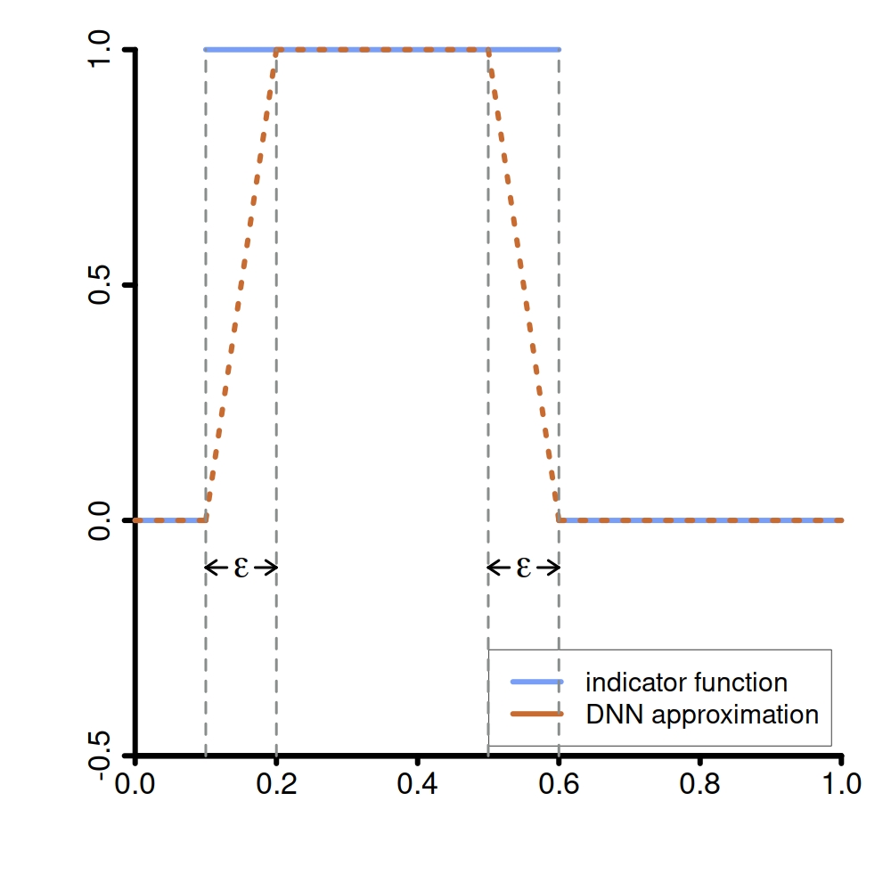
Figure 2: Left. Approximation 𝟏A(ε)\bm{1}_{A}^{(\varepsilon)} (orange) of the indicator function 𝟏A\bm{1}_{A} for A=[0.05,0.45]A=[0.05,0.45] (blue) according to Lemma 3.3 for ε=0.1\varepsilon=0.1 on X=[0,1]X=[0,1]. The construction of 𝟏A(ε)\bm{1}_{A}^{(\varepsilon)} ensures that 𝟏A(ε)\bm{1}_{A}^{(\varepsilon)} coincides with 𝟏A\bm{1}_{A} modulo a small set that is controlled by ε>0\varepsilon>0. Right. A DNN (orange) for regression that approximates the histogram 𝟏[0,0.5)+0.8⋅𝟏[0.5,1)\bm{1}_{[0,0.5)}+0.8\cdot\bm{1}_{[0.5,1)} and a DNN (green) that additionally tries to interpolate two samples x1=0.15x_{1}=0.15 and x2=0.975x_{2}=0.975 (located at the two vertical dotted lines) with yi=−0.5y_{i}=-0.5. The label y1y_{1} is correctly interpolated since the alignment condition (11) is satisfied for x1x_{1} with t=0.15t=0.15 and ε=δ=t/3=0.05\varepsilon=\delta=t/3=0.05 as in Example 3.6. In contrast, y2y_{2} is not correctly interpolated since condition (11) is violated for this tt and hence ε\varepsilon and δ\delta are too large.

Figure 2 illustrates 𝟏A(ε)\bm{1}_{A}^{(\varepsilon)} for d=1d=1. Moreover, the proof of Lemma D.3 shows that out of the 2​d22d^{2} weight parameters of the first layer, only 2​d2d are non-zero. In addition, the 2​d2d weight parameters of the neuron in the second layer are all identical. In order to approximate inflated histograms we need to know how to combine several functions of the form provided by Lemma 3.3 into a single neural network. An appealing feature of our DNNs is that the concatenation of layer structures is very easy.

Lemma 3.4.

If c∈ℝc\in\mathbb{R}, (p1,p2)∈ℕ2(p_{1},p_{2})\in\mathbb{N}^{2}, and g∈𝒜pg\in{\mathcal{A}}_{p}, g′∈𝒜p′g^{\prime}\in{\mathcal{A}}_{p^{\prime}}, then c​g∈𝒜pcg\in{\mathcal{A}}_{p} and g+g′∈𝒜p+p′g+g^{\prime}\in{\mathcal{A}}_{p+p^{\prime}}.

For an extended version of this result, see Lemma D.2. In particular, our constructed DNNs have a particularly sparse structure and the number of required neurons behaves in a very controlled and natural fashion.

With these insights, we are now able to find a representation similar to (4). To this end, we choose a cubic partition 𝒜=(Aj)j∈J{\mathcal{A}}=(A_{j})_{j\in J} of XX with width s>0s>0 and define for ε∈(0,s3]\varepsilon\in(0,\frac{s}{3}]

ℋ𝒜(ε):={∑j∈Jcj​ 1Aj(ε):cj∈Y},\displaystyle{\mathcal{H}}^{(\varepsilon)}_{{\cal A}}:=\biggl\{\sum_{j\in J}c_{j}\;\bm{1}_{A_{j}}^{(\varepsilon)}\;:\;c_{j}\in Y\biggr\}\,,

where 𝟏Aj(ε):=(𝟏Bj(ε))|Aj\bm{1}_{A_{j}}^{(\varepsilon)}:=(\bm{1}_{B_{j}}^{(\varepsilon)})_{|A_{j}} is the restriction of 𝟏Bj(ε)\bm{1}_{B_{j}}^{(\varepsilon)} to AjA_{j} and 𝟏Bj(ε)\bm{1}_{B_{j}}^{(\varepsilon)} is an ε\varepsilon-approximation of 𝟏Bj\bm{1}_{B_{j}} of Lemma 3.3. Here, BjB_{j} is the cell with Aj=Bj∩XA_{j}=B_{j}\cap X, see the text around (8). We call any function in ℋ𝒜(ε){\mathcal{H}}^{(\varepsilon)}_{{\cal A}} an ε\varepsilon-approximate histogram.

Our considerations above show that we have ℋ𝒜(ε)⊂𝒜p1,p2{\mathcal{H}}^{(\varepsilon)}_{{\cal A}}\subset{\mathcal{A}}_{p_{1},p_{2}} with p1=2​d​|J|p_{1}=2d|J| and m2=|J|m_{2}=|J|. Thus, any ε\varepsilon-approximate histogram can be represented by a neural network with 22 hidden layers. Inflated versions are now straightforward.

Definition 3.5.

Let s∈(0,1]s\in(0,1], m≥1m\geq 1, and ε∈(0,s/3]\varepsilon\in(0,s/3]. Then a function f:X→Yf:X\to Y is called an ε\varepsilon-approximated mm-inflated histogram of width ss if there exist a subset {x1∗,…,xm∗}∈Potm​(X)\{x_{1}^{*},...,x_{m}^{*}\}\in\mathrm{Pot}_{m}(X) and a cubic partition 𝒜{\cal A} of width ss that is properly aligned to {x1∗,…,xm∗}\{x_{1}^{*},...,x_{m}^{*}\} with parameter r∈[0,s)r\in[0,s) such that

f(ε)=h(ε)+∑i=1mbi​𝟏xi∗+t​B∞(δ),f^{(\varepsilon)}=h^{(\varepsilon)}+\sum_{i=1}^{m}b_{i}\bm{1}^{(\delta)}_{x_{i}^{*}+tB_{\infty}}\;,

where h(ε)∈ℋ𝒜(ε)h^{(\varepsilon)}\in{\mathcal{H}}_{\mathcal{A}}^{(\varepsilon)}, t∈(0,r]t\in(0,r], δ∈(0,t/3]\delta\in(0,t/3], bi∈2​Yb_{i}\in 2Y and where Ixi∗+t​B∞(δ)I^{(\delta)}_{x_{i}^{*}+tB_{\infty}} is a δ\delta-approximation of 𝟏xi∗+t​B∞\bm{1}_{x_{i}^{*}+tB_{\infty}} for all i=1,…,mi=1,...,m. We denote the set of all ε\varepsilon-approximated mm-inflated histograms of width ss by ℱs,m(ε){\mathcal{F}}^{(\varepsilon)}_{s,m}.

A short calculation shows that ℱs,m(ε)⊂𝒜p1,p2{\mathcal{F}}^{(\varepsilon)}_{s,m}\subset{\mathcal{A}}_{p_{1},p_{2}} with p1=2​d​(m+|J|)p_{1}=2d(m+|J|), p2=m+|J|p_{2}=m+|J| and |J|≤(2/s)d|J|\leq(2/s)^{d}. With these preparations, we can now introduce good and bad interpolating DNNs.

Example 3.6 (Good and bad interpolating DNN).

Let LL be the least squares loss, s∈(0,1]s\in(0,1] be a cell width and let ρ>0\rho>0 be an inflation parameter. For a data set D=((x1,yi),…,(xn,yn))D=((x_{1},y_{i}),\dots,(x_{n},y_{n})) we consider again a cubic partition 𝒜D=πm,s​(DX){\mathcal{A}}_{D}=\pi_{m,s}(D_{X}), with m=|DX|m=|D_{X}|, being properly aligned to DXD_{X} with parameter rr. Set t:=min⁡{r,ρ}t:=\min\{r,\rho\}. According to Example 2.8, a good interpolating HR is given by

fD,s,ρ+:=∑j∈Jcj+​𝟏Aj+∑i=1mbi+​𝟏xi∗+t​B∞,f_{D,s,\rho}^{+}:=\sum_{j\in J}c_{j}^{+}\bm{1}_{A_{j}}+\sum_{i=1}^{m}b^{+}_{i}\bm{1}_{x_{i}^{*}+tB_{\infty}}\;,

where the (cj+)j∈J(c_{j}^{+})_{j\in J} are given in (6) and b1+,…,bm+b^{+}_{1},\dots,b_{m}^{+} are from (14). For ε:=δ:=t/3\varepsilon:=\delta:=t/3 we then define the good interpolating DNN by

gD,s,ρ+=∑j∈Jcj+​𝟏Aj(ε)+∑i=1mbi+​𝟏xi∗+t​B∞(δ).g_{D,s,\rho}^{+}=\sum_{j\in J}c_{j}^{+}\bm{1}^{(\varepsilon)}_{A_{j}}+\sum_{i=1}^{m}b^{+}_{i}\bm{1}^{(\delta)}_{x_{i}^{*}+tB_{\infty}}\,.

Clearly, we have gD,s,ρ+∈ℱs,m(ε)g_{D,s,\rho}^{+}\in{\mathcal{F}}^{(\varepsilon)}_{s,m}. We call the map D↦gD,s,ρ+D\mapsto g_{D,s,\rho}^{+} a good interpolating DNN and it is easy to see that this network indeed interpolates DD. Finally, the bad interpolating DNN gD,s,ρ−g_{D,s,\rho}^{-} is defined analogously using the bad interpolating HR from Example 2.9, instead.

Similarly to our inflated histograms from the previous section, the next theorem shows that the good interpolating DNN is consistent while the bad interpolating DNN fails to be. The proof of this result is given in Appendix D.3.

Theorem 3.7 ((Non)-consistency).

Let LL be the least-squares loss and let D∈(X×Y)nD\in(X\times Y)^{n} be an i.i.d. sample of size n≥1n\geq 1. Let D↦gD,s,ρ+D\mapsto g_{D,s,\rho}^{+} denote the good interpolating DNN from Example 3.6. Similarly, let D↦gD,s,ρ−D\mapsto g_{D,s,\rho}^{-} denote the bad interpolating DNN from Example 3.6. Assume that (sn)n∈ℕ(s_{n})_{n\in\mathbb{N}} is a sequence with sn→0s_{n}\rightarrow 0, ln⁡(n​snd)n​snd→0\frac{\ln(ns_{n}^{d})}{ns_{n}^{d}}\to 0 as n→∞n\to\infty as well as sn>2n−1/ds_{n}>2n^{-1/d}. Additionally, let (ρn)n∈ℕ(\rho_{n})_{n\in\mathbb{N}} be a non-negative sequence with ρn≤2n−1/d\rho_{n}\leq 2n^{-1/d}. Then gD,sn,ρn±∈𝒜4​d​n,2​ng_{D,s_{n},\rho_{n}}^{\pm}\in{\mathcal{A}}_{4dn,2n}. Moreover, for all distributions PP that satisfy Assumption 2.10 for a function φ\varphi with ρn−d​φ​(ρn)→0\rho_{n}^{-d}\varphi(\rho_{n})\to 0 for n→∞n\to\infty, we have

‖gD,sn,ρn+−fL,P∗‖L2​(PX)→0,\displaystyle||g_{D,s_{n},\rho_{n}}^{+}-{f_{L,P}^{*}}||_{L_{2}(P_{X})}\to 0\,, (30)
‖gD,sn,ρn−−fL,P†‖L2​(PX)→0,\displaystyle||g_{D,s_{n},\rho_{n}}^{-}-{f_{L,P}^{\dagger}}||_{L_{2}(P_{X})}\to 0\,, (31)

in probability for |D|→∞|D|\to\infty.

The above result can further be refined to establishing rates of convergence if the width sns_{n} and the inflation parameter ρn\rho_{n} converge to zero sufficiently fast as n→∞n\to\infty. The proof is provided in Appendix D.4.

Theorem 3.8 (Learning Rates).

Let LL be the least-squares loss and let D∈(X×Y)nD\in(X\times Y)^{n} be an i.i.d. sample of size n≥1n\geq 1. Let D↦gD,s,ρ+D\mapsto g_{D,s,\rho}^{+} denote the good interpolating DNN from Example 3.6. Similarly, let D↦gD,s,ρ−D\mapsto g_{D,s,\rho}^{-} denote the bad interpolating DNN from Example 3.6. Suppose that fL,P∗{f_{L,P}^{*}} is α\alpha-Hölder continuous with α∈(0,1]\alpha\in(0,1] and that PP satisfies Assumption 2.10 for some function φ\varphi. Assume further that (sn)n∈ℕ(s_{n})_{n\in\mathbb{N}} is a sequence with

sn=n−γ,γ=12​α+ds_{n}=n^{-\gamma}\;,\quad\gamma=\frac{1}{2\alpha+d}

and that (ρn)n≥1(\rho_{n})_{n\geq 1} is a non-negative sequence with ρn≤2n−1/d\rho_{n}\leq 2n^{-1/d} and ρn−dφ(ρn)≤ln(n)n−2/3\rho_{n}^{-d}\varphi(\rho_{n})\leq\ln(n)n^{-2/3} for all n≥1n\geq 1. Then there exists a constant cd,α>0c_{d,\alpha}>0 only depending on dd, α\alpha, and |fL,P∗|α|f^{*}_{L,P}|_{\alpha}, such that for all n≥2n\geq 2 the good interpolating histogram rule satisfies

‖gD,sn,ρn+−fL,P∗‖L2​(PX)\displaystyle||g_{D,s_{n},\rho_{n}}^{+}-{f_{L,P}^{*}}||_{L_{2}(P_{X})} ≤cα,d​ln⁡(n)​(1n)α​γ,\displaystyle\leq c_{\alpha,d}\sqrt{\ln(n)}\left(\frac{1}{n}\right)^{\alpha\gamma}\;, (32)

with probability PnP^{n} not less than 1−2d​n1+d​e−nd​γ1-2^{d}n^{1+d}e^{-n^{d\gamma}}. Furthermore, for all n≥2n\geq 2, the bad interpolating histogram rule satisfies

‖gD,sn,ρn−−fL,P†‖L2​(PX)\displaystyle||g_{D,s_{n},\rho_{n}}^{-}-{f_{L,P}^{\dagger}}||_{L_{2}(P_{X})} ≤cα,d​ln⁡(n)​(1n)α​γ.\displaystyle\leq c_{\alpha,d}\sqrt{\ln(n)}\left(\frac{1}{n}\right)^{\alpha\gamma}\;. (33)

with probability PnP^{n} not less than 1−2d​n1+d​e−nd​γ1-2^{d}n^{1+d}e^{-n^{d\gamma}}. Finally, there exists a natural number nd,α>0n_{d,\alpha}>0 such that for any n≥nd,αn\geq n_{d,\alpha} we have gD,sn,ρn±∈𝒜4​d​n,2​ng_{D,s_{n},\rho_{n}}^{\pm}\in{\mathcal{A}}_{4dn,2n}.

Note that the rates of convergence in (32) and (33) remain true if we consider a sequence sns_{n} with c−1​n−γ≤sn≤c​n−γc^{-1}n^{-\gamma}\leq s_{n}\leq cn^{-\gamma} for some constant cc independent of nn. In fact, the only reason why we have formulated Theorem 3.8 with sn=n−γs_{n}=n^{-\gamma} is to avoid another constant appearing in the statements. Moreover, if we choose sn:=2​a​⌊n−γ⌋−1s_{n}:=2a\lfloor n^{-\gamma}\rfloor^{-1} with a:=31/d/(31/d−2)a:=3^{1/d}/(3^{1/d}-2), then we have |J|≤(2​sn−1+2)d≤(a−1​n1/d+2)d≤n|J|\leq(2s_{n}^{-1}+2)^{d}\leq(a^{-1}n^{1/d}+2)^{d}\leq n for all n≥3n\geq 3. Consequently, for m:=nm:=n, we can choose nd,α:=3n_{d,\alpha}:=3, and hence we have gD,sn,ρn±∈𝒜4​d​n,2​ng_{D,s_{n},\rho_{n}}^{\pm}\in{\mathcal{A}}_{4dn,2n} for all n≥3n\geq 3 while (32) and (33) hold true modulo a change in the constant cα,dc_{\alpha,d}.

Discussion of results. To fully appreciate Theorems 3.7 and 3.8 as well as their underlying construction let us discuss its various consequences:

First, the good interpolating DNN predictors gD,sn,ρn+g_{D,s_{n},\rho_{n}}^{+} show that its is actually possible to train sufficiently large, over-parameterized DNNs such that they become consistent and enjoy optimal learning rates up to a logrithmic factor without adapting the network size to the particular smoothness of the target function. In fact, it suffices to consider DNNs with two hidden layers and 4​d​n4dn, respectively 2​n2n neurons in the first, respectively second, hidden layer. In other words, Theorems 3.7 and 3.8 already apply to moderately over-parameterized DNNs, and by the particular properties of the ReLU-activation function, also for all larger network architectures. In addition, when using architectures of minimal size, training, that is constructing gD,sn,ρn+g_{D,s_{n},\rho_{n}}^{+}, can be done in 𝒪⁡(d2⋅n2){\cal O}(d^{2}\cdot n^{2})-time if the DNNs are implemented as fully connected networks. Moreover, the constructed DNNs have a particularly sparse structure and exploiting this can actually reduce the training time to 𝒪⁡(d⋅n⋅log⁡n){\cal O}(d\cdot n\cdot\log n). While we believe that this is one of the very first statistically sound end-to-end22 2 By “end-to-end” we mean the explicit construction of an efficient, feasible, and implementable training algorithm and the rigorous statistical analysis of this very particular algorithm under minimal assumptions. proofs of consistency and optimal rates for DNNs, we also need to admit that our training algorithm is mostly interesting from a theoretical point of view, but useless for practical purposes.

Second, Theorems 3.7 and 3.8 also have its consequences for DNNs trained by variants of stochastic gradient descent (SGD) if the resulting predictor is interpolating. Indeed, these theorems show that ending in a global minimum may result in either a very good learning behavior or an extremely overfitting, bad behavior. In fact, all the observations made for histograms at the end of Section 2 apply to DNNs, too. In particular, since for n≥nd,αn\geq n_{d,\alpha} the 𝒜4​d​n,2​n{\mathcal{A}}_{4dn,2n}-networks can ε\varepsilon-approximate all functions in ℱs,n∗{\cal F}_{s,n}^{*} for all ε≥0\varepsilon\geq 0 and all s∈[n−1/d,1]s\in[n^{-1/d},1], we can, for example, find, for each polynomial learning rate slower than n−α​γn^{-\alpha\gamma}, an interpolating learning method D↦fDD\mapsto f_{D} with fD∈𝒜4​d​n,2​nf_{D}\in{\mathcal{A}}_{4dn,2n} that learns with this rate. Similarly, we can find interpolating fD∈𝒜4​d​n,2​nf_{D}\in{\mathcal{A}}_{4dn,2n} with various degrees of bad learning behavior. In summary, the optimization landscape induced by 𝒜4​d​n,2​n{\mathcal{A}}_{4dn,2n} contains a wide variety of global minima whose learning properties range somewhat continuously from essentially optimal to extremely poor. Consequently, an optimization guarantee for (S)GD, that is, a guarantee that (S)GD finds a global minimum in the optimization landscape, is useless for learning guarantees unless more information about the particular nature of the minimum found is provided. Moreover, it becomes clear that considering (S)GD without the initialization of the weights and biases is a meaningless endeavor: For example, constructing gD,sn,ρn±g_{D,s_{n},\rho_{n}}^{\pm} can be viewed as a very particular form of initilization for which (S)GD won’t change the parameters anymore. More generally, when initializing the parameters randomly in the attraction basin of gD,sn,ρn±g_{D,s_{n},\rho_{n}}^{\pm} then GD will converge to gD,sn,ρn±g_{D,s_{n},\rho_{n}}^{\pm} and therefore the behavior of GD is completely determined by the initialization. In this respect note that so far there is no statistically sound way to distinguish between good and bad interpolating DNNs on the basis of the training set alone, and hence the only way to identify good interpolating DNNs obtained by SGD is to use a validation set. Now, for the good interpolating DNNs of Theorem 3.7 it is actually possible to construct a finite set of candidates such that the one with the best validation error achieves the optimal learning rates without knowing α\alpha. For DNNs trained by SGD, however, we do not have this luxury anymore. Indeed, while we can still identify the best predicting DNN from a finite set of SGD-learned interpolating DNNs we no longer have any theoretical understanding of whether there is any useful candidate among them, or whether they all behave like a gD,sn,ρn−g_{D,s_{n},\rho_{n}}^{-}.

Third, for both consistency and learning with essentially optimal rates it is by no means necessary to find a global minimum, or at least a local minimum, in the optimization landscape. For example, the positive learning rates (25) also hold for ordinary cubic histograms with widths sn:=n−γs_{n}:=n^{-\gamma}, and the latter can, of course, also be approximated by 𝒜4​d​n,2​n{\mathcal{A}}_{4dn,2n}. Repeating the proof of Theorem 3.8 it is easy to verify that these approximations also enjoy the good learning rates (32). Moreover, these approximations fDf_{D} are almost never global minima, or more precisely, fDf_{D} is not a global minimum as soon as there exist a cubic cell AA containing two samples xix_{i} and xjx_{j} with different labels, i.e. yi≠yjy_{i}\neq y_{j}. In fact, in this case, fDf_{D} is not even a local minimum. To see this, assume without loss of generality that xix_{i} is one of the samples in AA with yi≠fD​(xi)y_{i}\neq f_{D}(x_{i}). Considering fD,λ:=fD+λ​bi+​𝟏xi+t​B∞(t/3)f_{D,\lambda}:=f_{D}+\lambda b_{i}^{+}\bm{1}_{x_{i}+tB_{\infty}}^{(t/3)} for all λ∈[0,1]\lambda\in[0,1] and t:=min⁡{r,ρ}t:=\min\{r,\rho\} we then see that there is a continuous path in the parameter space of 𝒜4​d​n,2​n{\mathcal{A}}_{4dn,2n} that corresponds to the ∥⋅∥∞\|\cdot\|_{\infty}-continuous path λ↦fD,λ\lambda\mapsto f_{D,\lambda} in the set of functions 𝒜4​d​n,2​n{\mathcal{A}}_{4dn,2n} for which we have ℛL,D​(fD,λ)<ℛL,D​(fD){{\cal R}_{L,D}(f_{D,\lambda})}<{{\cal R}_{L,D}(f_{D})} for all λ∈(0,1]\lambda\in(0,1]. In other words, fDf_{D} is not a local minimum. In this respect we note that this phenomenon also occurs to some extend in under-parameterized DNNs, at least for d=1d=1. Indeed, if we consider m:=1m:=1 and sn:=nγs_{n}:=n^{\gamma}, then fD,fD,λ∈𝒜4​d​nγ​d,2​nγ​df_{D},f_{D,\lambda}\in{\mathcal{A}}_{4dn^{\gamma d},2n^{\gamma d}} for all sufficiently large nn. Now, the functions in 𝒜4​d​nγ​d,2​nγ​d{\mathcal{A}}_{4dn^{\gamma d},2n^{\gamma d}} have 𝒪⁡(d2​n2​γ​d){\cal O}(d^{2}n^{2\gamma d}) many parameters and for 2​γ​d=2​d2​α+d<12\gamma d=\frac{2d}{2\alpha+d}<1, that is α>d/2=1/2\alpha>d/2=1/2, we then see that we have strictly less than 𝒪⁡(n){\cal O}(\sqrt{n}) neurons with 𝒪⁡(n){\cal O}(n) parameters, while all the observations made so far still hold.

References

  • [1] Zeyuan Allen-Zhu, Yuanzhi Li, and Yingyu Liang. Learning and generalization in overparameterized neural networks, going beyond two layers. In Proceedings of the 33rd International Conference on Neural Information Processing Systems, pages 6158–6169, 2019.
  • [2] Peter L Bartlett, Philip M Long, Gábor Lugosi, and Alexander Tsigler. Benign overfitting in linear regression. Proceedings of the National Academy of Sciences, 117(48):30063–30070, 2020.
  • [3] H. Bauer. Measure and Integration Theory. De Gruyter, Berlin, 2001.
  • [4] M. Belkin, D. J. Hsu, and P. Mitra. Overfitting or perfect fitting? Risk bounds for classification and regression rules that interpolate. In S. Bengio, H. Wallach, H. Larochelle, K. Grauman, N. Cesa-Bianchi, and R. Garnett, editors, Advances in Neural Information Processing Systems 31, pages 2300–2311. Curran Associates, Inc., 2018.
  • [5] Mikhail Belkin, Daniel Hsu, and Ji Xu. Two models of double descent for weak features. SIAM Journal on Mathematics of Data Science, 2(4):1167–1180, 2020.
  • [6] Mikhail Belkin, Alexander Rakhlin, and Alexandre B Tsybakov. Does data interpolation contradict statistical optimality? In The 22nd International Conference on Artificial Intelligence and Statistics, pages 1611–1619. PMLR, 2019.
  • [7] Lin Chen, Yifei Min, Mikhail Belkin, and Amin Karbasi. Multiple descent: Design your own generalization curve. arXiv preprint arXiv:2008.01036, 2020.
  • [8] L. Devroye, L. Györfi, and G. Lugosi. A Probabilistic Theory of Pattern Recognition. Springer, New York, 1996.
  • [9] I. Goodfellow, Y. Bengio, and A. Courville. Deep Learning. MIT Press, Cambridge, MA, 2016.
  • [10] L. Györfi, M. Kohler, A. Krzyżak, and H. Walk. A Distribution-Free Theory of Nonparametric Regression. Springer-Verlag, New York, 2002.
  • [11] J Hoffman-Jorgensen. Probability With a View Towards Statistics, Volume I. Routledge, 2017.
  • [12] Tengyuan Liang, Alexander Rakhlin, and Xiyu Zhai. On the multiple descent of minimum-norm interpolants and restricted lower isometry of kernels. In Conference on Learning Theory, pages 2683–2711. PMLR, 2020.
  • [13] S. Ma, R. Bassily, and M. Belkin. The power of interpolation: Understanding the effectiveness of SGD in modern over-parametrized learning. In J. Dy and A. Krause, editors, Proceedings of the 35th International Conference on Machine Learning, volume 80 of Proceedings of Machine Learning Research, pages 3325–3334, 2018.
  • [14] Song Mei and Andrea Montanari. The generalization error of random features regression: Precise asymptotics and the double descent curve. Communications on Pure and Applied Mathematics, 2019.
  • [15] Vaishnavh Nagarajan and J Zico Kolter. Uniform convergence may be unable to explain generalization in deep learning. arXiv preprint arXiv:1902.04742, 2019.
  • [16] Behnam Neyshabur, Zhiyuan Li, Srinadh Bhojanapalli, Yann LeCun, and Nathan Srebro. Towards understanding the role of over-parametrization in generalization of neural networks. In International Conference on Learning Representations (ICLR), 2019.
  • [17] R. Salakhutdinov. Deep learning tutorial at the Simons Institute, 2017. https://simons.berkeley.edu/talks/ruslan-salakhutdinov-01-26-2017-1.
  • [18] S. Shalev-Shwartz and S. Ben-David. Understanding Machine Learning: From Theory to Algorithms. Cambridge University Press, Cambridge, 2014.
  • [19] I. Steinwart and A. Christmann. Support Vector Machines. Springer, New York, 2008.
  • [20] Alexander Tsigler and Peter L Bartlett. Benign overfitting in ridge regression. arXiv preprint arXiv:2009.14286, 2020.
  • [21] A. B. Tsybakov. Introduction to Nonparametric Estimation. Springer-Verlag, New York, 2009.
  • [22] S. van de Geer. Applications of Empirical Process Theory. Cambridge University Press, Cambridge, 2000.
  • [23] V. N. Vapnik. Statistical Learning Theory. John Wiley & Sons, New York, 1998.
  • [24] C. Zhang, S. Bengio, M. Hardt, B. Recht, and O. Vinyals. Understanding deep learning requires rethinking generalization. Technical report, 2016. http://arxiv.org/abs/1611.03530.
  • [25] Lijia Zhou, DJ Sutherland, and Nati Srebro. On uniform convergence and low-norm interpolation learning. Advances in Neural Information Processing Systems, 33, 2020.

Appendix A Characterization of empirical risk minimizers

In this section we briefly provide a full characterization of empirical risk minimizers that we use several times for proving our main results.

Lemma A.1 (Characterization of ERMs).

Let YY be convex, A⊆XA\subseteq X be non-empty, 𝒜=(Aj)j∈J{\cal A}=(A_{j})_{j\in J} be a finite partition of AA, and

ℋ𝒜:={∑j∈Jcj​𝟏Aj:cj∈Y}.{\cal H}_{{\cal A}}:=\biggl\{\sum_{j\in J}c_{j}\bm{1}_{A_{j}}:c_{j}\in Y\biggr\}\;.

Moreover, let D=((x1,y1),…,(xn,yn))∈(X×Y)nD=((x_{1},y_{1}),\dots,(x_{n},y_{n}))\in(X\times Y)^{n} be a data set and let LA​(x,y,t)=𝟏A​(x)​L​(y,t)L_{A}(x,y,t)=\bm{1}_{A}(x)L(y,t), with LL being the least squares loss. Furthermore, denote the number of samples whose covariates fall into cell AjA_{j} by NjN_{j}, that is Nj:=|{i:xi∈Aj}|N_{j}:=|\{i:x_{i}\in A_{j}\}|. Then, for every f∗∈ℋ𝒜f^{*}\in{\cal H}_{{\cal A}} with representation f∗=∑j∈Jcj​𝟏Ajf^{*}=\sum_{j\in J}c_{j}\bm{1}_{A_{j}}, the following statements are equivalent:

  1. i)

    The function f∗f^{*} is an empirical risk minimizer, that is

    ℛLA,D​(f∗)=minf∈ℋ𝒜⁡ℛLA,D​(f).{{\cal R}_{L_{A},D}(f^{*})}=\min_{f\in{\cal H}_{{\cal A}}}{{\cal R}_{L_{A},D}(f)}\,.
  2. ii)

    For all j∈Jj\in J satisfying Nj≠0N_{j}\neq 0 we have

    cj=1Nj∑i:xi∈Ajyi.\displaystyle c_{j}=\frac{1}{N_{j}}\sum_{i:x_{i}\in A_{j}}y_{i}\;. (34)

Proof of of Lemma A.1: We first note that for an f∗∈ℋ𝒜f^{*}\in{\cal H}_{{\cal A}} with representation f∗=∑j∈Jcj​𝟏Ajf^{*}=\sum_{j\in J}c_{j}\bm{1}_{A_{j}} we have

ℛLA,D(f∗)=1n∑i=1n𝟏A(xi)L(yi,f∗(xi))=1n∑j∈J∑i:xi∈AjL(yi,cj).\displaystyle{{\cal R}_{L_{A},D}(f^{*})}=\frac{1}{n}\sum_{i=1}^{n}\bm{1}_{A}(x_{i})L\bigl(y_{i},f^{*}(x_{i})\bigr)=\frac{1}{n}\sum_{j\in J}\sum_{i:x_{i}\in A_{j}}L(y_{i},c_{j})\,.

Consequently, f∗f^{*} is an empirical risk minimizer, if and only if cjc_{j} minimizes ∑i:xi∈AjL(yi,⋅)\sum_{i:x_{i}\in A_{j}}L(y_{i},\cdot) for all j∈Jj\in J. Now, if Nj=0N_{j}=0, the sum is empty, and hence there is nothing to consider. For j∈Jj\in J with NjN_{j} we observe that

∑i:xi∈AjL(yi,cj)=Njcj2−2cj(∑i:xi∈Ajyi)+∑i:xi∈Ajyi2,\sum_{i:x_{i}\in A_{j}}L(y_{i},c_{j})=N_{j}c_{j}^{2}-2c_{j}\biggl(\sum_{i:x_{i}\in A_{j}}y_{i}\biggr)+\sum_{i:x_{i}\in A_{j}}y_{i}^{2}\,,

which is minimized for cjc_{j} given by (34). ∎

Appendix B Existence of properly aligned cubic partitioning rule

In this section we prove the existence of a properly aligned cubic partitioning rule.

Proof of Theorem 2.5: Recall that cubic partitions ℬ{\cal B} of ℝd\mathbb{R}^{d} have a representation of the form (8). Now, to construct πm,s\pi_{m,s} we will consider a finite set of candidate offsets x1†,…,xK†∈ℝdx_{1}^{\dagger},\dots,x_{K}^{\dagger}\in\mathbb{R}^{d}. For the construction of these offsets we write δ:=s/(m+1)\delta:=s/(m+1) and for j∈{0,…,m}j\in\{0,\dots,m\} we further define

zj†:=(j+12)​δ.z_{j}^{\dagger}:=\Bigl(j+\frac{1}{2}\Bigr)\,\delta\,.

Now, our candidate offsets x1†,…,xK†∈ℝdx_{1}^{\dagger},\dots,x_{K}^{\dagger}\in\mathbb{R}^{d} are exactly those vectors whose coordinates are taken from z0†,…,zm†z_{0}^{\dagger},\dots,z_{m}^{\dagger}. Clearly, this gives K=(m+1)dK=(m+1)^{d}. Now let {x1∗,…,xm∗}∈Potm​([−1,1]d)\{x_{1}^{*},\dots,x_{m}^{*}\}\in\mathrm{Pot}_{m}([-1,1]^{d}). In the following, we will identify the offset xℓ†x_{\ell}^{\dagger} that leads to πm,s​({x1∗,…,xm∗})\pi_{m,s}(\{x_{1}^{*},\dots,x_{m}^{*}\}) coordinate-wise. We begin by determining its first coordinate xℓ,1†x_{\ell,1}^{\dagger}. To this end, we define

Ij:=⋃k∈ℤ[ks+jδ,ks+(j+1)δ).I_{j}:=\bigcup_{k\in\mathbb{Z}}\bigr[ks+j\delta,\,ks+(j+1)\delta\bigl)\,.

Our first goal is to show that I0,…,ImI_{0},\dots,I_{m} are a partition of ℝ\mathbb{R}. To this end, we fix an x∈ℝx\in\mathbb{R}. Then there exists a unique k∈ℤk\in\mathbb{Z} with k​s≤x<(k+1)​sks\leq x<(k+1)s. Moreover, for y:=x−k​s∈[0,s)y:=x-ks\in[0,s), there exists a unique j∈{0,…,m}j\in\{0,\dots,m\} with j​δ≤y<(j+1)​δj\delta\leq y<(j+1)\delta. Consequently, we have found x∈[ks+jδ,ks+(j+1)δ)x\in[ks+j\delta,\,ks+(j+1)\delta). This shows ℝ⊂I0∪⋯∪Im\mathbb{R}\subset I_{0}\cup\dots\cup I_{m}, and the converse inclusion is trivial. Let us now fix some j,j′∈{0,…,m}j,j^{\prime}\in\{0,\dots,m\} and assume that there is an x∈Ij∩Ij′x\in I_{j}\cap I_{j^{\prime}}. Then there exist k,k′∈ℤk,k^{\prime}\in\mathbb{Z} such that

x∈[ks+jδ,ks+(j+1)δ)∩[k′s+j′δ,k′s+(j′+1)δ).\displaystyle x\in\bigr[ks+j\delta,\,ks+(j+1)\delta\bigl)\,\cap\,\bigr[k^{\prime}s+j^{\prime}\delta,\,k^{\prime}s+(j^{\prime}+1)\delta\bigl)\,. (35)

Since (j+1)​δ≤s(j+1)\delta\leq s and (j′+1)​δ≤s(j^{\prime}+1)\delta\leq s, we conclude that k​s≤x<(k+1)​sks\leq x<(k+1)s and k′​s≤x<(k′+1)​sk^{\prime}s\leq x<(k^{\prime}+1)s. As observed above this implies k=k′k=k^{\prime}. Now consider y:=x−k​s∈[0,s)y:=x-ks\in[0,s). Then (35) implies

y∈[jδ,(j+1)δ)∩[j′δ,(j′+1)δ),y\in\bigr[j\delta,\,(j+1)\delta\bigl)\,\cap\,\bigr[j^{\prime}\delta,\,(j^{\prime}+1)\delta\bigl)\,,

and again we have seen above that this implies j=j′j=j^{\prime}. This shows Ij∩Ij′=∅I_{j}\cap I_{j^{\prime}}=\emptyset for all j≠j′j\neq j^{\prime}.

Let us now denote the first coordinate of xi∗x_{i}^{*} by xi,1∗x_{i,1}^{*}. Then DX,1∗:={xi,1∗:i=1,…,m}D_{X,1}^{*}:=\{x_{i,1}^{*}:i=1,\dots,m\} satisfies |DX,1∗|≤m|D_{X,1}^{*}|\leq m and since we have m+1m+1 cells IjI_{j}, we conclude that there exists a j1∗∈{0,…,m}j_{1}^{*}\in\{0,\dots,m\} with DX,1∗∩Ij1∗=∅D_{X,1}^{*}\cap I_{j_{1}^{*}}=\emptyset. We define

xℓ,1†:=zj1∗†=(j1∗+12)​δ.x_{\ell,1}^{\dagger}:=z_{j_{1}^{*}}^{\dagger}=\Bigl(j_{1}^{*}+\frac{1}{2}\Bigr)\,\delta\,.

Next we repeat this construction for the remaining d−1d-1 coordinates, so that we finally obtain xℓ†:=(zj1∗†,…,zjd∗†)∈ℝdx_{\ell}^{\dagger}:=(z_{j_{1}^{*}}^{\dagger},\dots,z_{j_{d}^{*}}^{\dagger})\in\mathbb{R}^{d} for indices j1∗,…,jd∗∈{0,…,m}j_{1}^{*},\dots,j_{d}^{*}\in\{0,\dots,m\} found by the above reasoning.

It remains to show that (11) holds the cubic partition (8) with offset xℓ†x_{\ell}^{\dagger} and all t>0t>0 with t≤s3​m+3=δ/3t\leq\frac{s}{3m+3}=\delta/3. To this end, we fix an xi∗x_{i}^{*}. Then its cell B⁡(xi∗)B(x_{i}^{*}) is described by a unique k:=(k1,…,kd)∈ℤdk:=(k_{1},\dots,k_{d})\in\mathbb{Z}^{d}, namely

B(xi∗)=[xℓ,1†+k1s,xℓ,1†+(k1+1)s)×⋯×[xℓ,d†+kds,xℓ,d†+(kd+1)s).B(x_{i}^{*})=\bigl[x_{\ell,1}^{\dagger}+k_{1}s,\,x_{\ell,1}^{\dagger}+(k_{1}+1)s\bigr)\times\dots\times\bigl[x_{\ell,d}^{\dagger}+k_{d}s,\,x_{\ell,d}^{\dagger}+(k_{d}+1)s\bigr)\,.

Let us now consider the first coordinate xi,1∗x_{i,1}^{*}. By construction we know that xi,1∗∉Ij1∗x_{i,1}^{*}\not\in I_{j_{1}^{*}} and

(j1∗+12)⋅δ+k1​s≤xi,1∗<(j1∗+12)⋅δ+(k1+1)​s.\displaystyle\Bigl(j_{1}^{*}+\frac{1}{2}\Bigr)\cdot\delta+k_{1}s\,\leq\,x_{i,1}^{*}\,<\,\Bigl(j_{1}^{*}+\frac{1}{2}\Bigr)\cdot\delta+(k_{1}+1)s\,. (36)

Now, xi,1∗∉Ij1∗x_{i,1}^{*}\not\in I_{j_{1}^{*}} implies

xi,1∗∉[(k1+1)s+j1∗δ,(k1+1)s+(j1∗+1)δ)x_{i,1}^{*}\not\in\bigr[(k_{1}+1)s+j_{1}^{*}\delta,\,(k_{1}+1)s+(j_{1}^{*}+1)\delta\bigl)

Since the right hand side of (36) excludes the case xi,1∗≥(k1+1)​s+(j1∗+1)​δx_{i,1}^{*}\geq(k_{1}+1)s+(j_{1}^{*}+1)\delta, we hence find

xi,1∗<(k1+1)​s+j1∗​δ=xℓ,1†+(k1+1)​s−δ/2.x_{i,1}^{*}<(k_{1}+1)s+j_{1}^{*}\delta=x_{\ell,1}^{\dagger}+(k_{1}+1)s-\delta/2\,.

This shows xi,1∗+r<xℓ,1†+(k1+1)​sx_{i,1}^{*}+r<x_{\ell,1}^{\dagger}+(k_{1}+1)s for all r∈[−t,t]r\in[-t,t]. To show that xi,1∗+r>xℓ,1†+k1​sx_{i,1}^{*}+r>x_{\ell,1}^{\dagger}+k_{1}s holds for all r∈[−t,t]r\in[-t,t] we first observe that xi,1∗∉Ij1∗x_{i,1}^{*}\not\in I_{j_{1}^{*}} also implies

xi,1∗∉[k1s+j1∗δ,k1s+(j1∗+1)δ).x_{i,1}^{*}\not\in\bigr[k_{1}s+j_{1}^{*}\delta,\,k_{1}s+(j_{1}^{*}+1)\delta\bigl)\,.

Now, the left hand side of (36) excludes the case xi,1∗<k1​s+j1∗​δx_{i,1}^{*}<k_{1}s+j_{1}^{*}\delta. Consequently, we have

xi,1∗≥k1​s+(j1∗+1)​δ=xℓ,1†+k1​s+δ/2\displaystyle x_{i,1}^{*}\geq k_{1}s+(j_{1}^{*}+1)\delta=x_{\ell,1}^{\dagger}+k_{1}s+\delta/2

and this yields xi,1∗+r>xℓ,1†+k1​sx_{i,1}^{*}+r>x_{\ell,1}^{\dagger}+k_{1}s for all r∈[−t,t]r\in[-t,t]. Finally, by repeating these considerations for the remaining d−1d-1 coordinates, we conclude that xi∗+t​B∞⊂B⁡(xi∗)x_{i}^{*}+tB_{\infty}\subset B(x_{i}^{*}). ∎

Appendix C Learning properties of inflated histograms

In this section we provide the proofs of the results for the good and bad interpolating histogram rules from Section 2.2. To this end let us introduce some more notation. For a measurable set AA and a loss L:Y×ℝ→[0,∞)L:Y\times\mathbb{R}\to[0,\infty) we therefore introduce the loss LA:X×Y×ℝ→[0,∞)L_{A}:X\times Y\times\mathbb{R}\to[0,\infty) by

OPENLA​(x,y,t))=𝟏A​(x)​L​(y,t).L_{A}(x,y,t))=\bm{1}_{A}(x)L(y,t)\;. (37)

Obviously, for any measurable function f:X→ℝf:X\to\mathbb{R} it holds

ℛLA,P​(f)=ℛLA,P​(𝟏A​f).{{\cal R}_{L_{A},P}(f)}={{\cal R}_{L_{A},P}(\bm{1}_{A}f)}\;. (38)

Moreover, by linearity, for every measurable sets B⊂AB\subset A, the risk then decomposes as

ℛLA,P​(f)=ℛLA∖B,P​(f)+ℛLB,P​(f).{{\cal R}_{L_{A},P}(f)}={\mathcal{R}}_{L_{A\setminus B},P}(f)+{\mathcal{R}}_{L_{B},P}(f)\;. (39)

The next result shows that also the Bayes risk enjoys a similar decomposition.

Lemma C.1.

Let A,B⊂XA,B\subset X be non-empty, disjoint, and measurable with A∪B=XA\cup B=X. Then we have

ℛL,P∗=ℛLA,P∗+ℛLB,P∗.{{\cal R}_{L,P}^{*}}={{\cal R}_{L_{A},P}^{*}}+{{\cal R}_{L_{B},P}^{*}}\,.

Proof of Lemma C.1: Basically, this is a consequence of the presence of the indicator functions 𝟏A,𝟏B\bm{1}_{A},\bm{1}_{B} in the definition of LA,LBL_{A},L_{B}, see (37). More precisely, there is a sequence of functions fnAf_{n}^{A} with {fnA≠0}⊂A\{f_{n}^{A}\neq 0\}\subset A such that

ℛLA,P​(fnA)→ℛLA,P∗,{{\cal R}_{L_{A},P}(f_{n}^{A})}\to{{\cal R}_{L_{A},P}^{*}}\;,

as n→∞n\to\infty, and similarly for AA replaced by BB. Thus, for fn:=fnA+fnBf_{n}:=f_{n}^{A}+f_{n}^{B}, one has

ℛL,P∗≤limn→∞ℛL,P​(fn)=limn→∞ℛLA,P​(fnA)+limn→∞ℛLB,P​(fnB)=ℛLA,P∗+ℛLB,P∗.{{\cal R}_{L,P}^{*}}\leq\lim_{n\to\infty}{{\cal R}_{L,P}(f_{n})}=\lim_{n\to\infty}{{\cal R}_{L_{A},P}(f_{n}^{A})}+\lim_{n\to\infty}{{\cal R}_{L_{B},P}(f_{n}^{B})}={{\cal R}_{L_{A},P}^{*}}+{{\cal R}_{L_{B},P}^{*}}\,.

Since the converse inequality is trivial, this proves the lemma. ∎

C.1 Preparatory Lemmata

The next lemma provides a bound on the difference of the risks of two measurable functions.

Lemma C.2.

Let Y=[−1,1]Y=[-1,1] and let f1,f2:X→Yf_{1},f_{2}:X\to Y be measurable functions. For A⊂XA\subset X measurable and non-empty we define LA​(x,y,t)=𝟏A​(x)​L​(y,t)L_{A}(x,y,t)=\bm{1}_{A}(x)L(y,t) with LL being the least square loss. Then the following two inequalities hold:

|ℛLA,P​(f1)−ℛLA,P​(f2)|\displaystyle\bigl|{{\cal R}_{L_{A},P}(f_{1})}-{{\cal R}_{L_{A},P}(f_{2})}\bigr| ≤4PX(A∩{f1≠f2}),\displaystyle\leq 4\;P_{X}\bigl(A\cap\{f_{1}\neq f_{2}\}\bigr)\;,
‖𝟏A​(f1−f2)‖L2​(PX)2\displaystyle||\bm{1}_{A}(f_{1}-f_{2})||^{2}_{L_{2}(P_{X})} ≤4PX(A∩{f1≠f2}).\displaystyle\leq 4\;P_{X}\bigl(A\cap\{f_{1}\neq f_{2}\}\bigr)\;.

Proof of Lemma C.2: We begin by proving the first inequality. To this end, we note that the definition of LL yields

ℛL,P​(f1)−ℛL,P​(f2)\displaystyle{{\cal R}_{L,P}(f_{1})}-{{\cal R}_{L,P}(f_{2})} =∫A∫Y(y−f1​(x))2−(y−f2​(x))2​P​(𝑑y|x)​d​PX​(x)\displaystyle=\int_{A}\int_{Y}(y-f_{1}(x))^{2}-(y-f_{2}(x))^{2}\,P(dy|x)dP_{X}(x)
=∫A∩{f1≠f2}∫Y(y−f1(x))2−(y−f2(x))2P(dy|x)dPX(x).\displaystyle=\int_{A\cap\{f_{1}\neq f_{2}\}}\int_{Y}(y-f_{1}(x))^{2}-(y-f_{2}(x))^{2}P(dy|x)dP_{X}(x)\;.

Now observe that y,fi​(x)∈[−1,1]y,f_{i}(x)\in[-1,1] implies (y−fi​(x))2≤4(y-f_{i}(x))^{2}\leq 4. Moreover, we also have (y−fi​(x))2≥0(y-f_{i}(x))^{2}\geq 0, and hence we conclude that

|(y−f1​(x))2−(y−f2​(x))2|≤4.\Bigl|(y-f_{1}(x))^{2}-(y-f_{2}(x))^{2}\Bigr|\leq 4\;.

Combining these considerations we find

|ℛL,P​(f1)−ℛL,P​(f2)|\displaystyle\bigl|{{\cal R}_{L,P}(f_{1})}-{{\cal R}_{L,P}(f_{2})}\bigr| ≤∫A∩{f1≠f2}∫Y|(y−f1(x))2−(y−f2(x))2|P(dy|x)dPX(x)\displaystyle\leq\int_{A\cap\{f_{1}\neq f_{2}\}}\int_{Y}\Bigl|(y-f_{1}(x))^{2}-(y-f_{2}(x))^{2}\Bigr|P(dy|x)dP_{X}(x)
≤4PX(A∩{f1≠f2}).\displaystyle\leq 4P_{X}\bigl(A\cap\{f_{1}\neq f_{2}\}\bigr)\;.

The second inequality can be show similarly. Namely, we have

‖𝟏A​(f1−f2)‖L2​(PX)2\displaystyle||\bm{1}_{A}(f_{1}-f_{2})||^{2}_{L_{2}(P_{X})} =∫A(f1​(x)−f2​(x))2​d​PX​(x)\displaystyle=\int_{A}(f_{1}(x)-f_{2}(x))^{2}dP_{X}(x)
=∫A∩{f1≠f2}(f1(x)−f2(x))2dPX(x)\displaystyle=\int_{A\cap\{f_{1}\neq f_{2}\}}(f_{1}(x)-f_{2}(x))^{2}dP_{X}(x)
≤4PX(A∩{f1≠f2}),\displaystyle\leq 4P_{X}\bigl(A\cap\{f_{1}\neq f_{2}\}\bigr)\;,

where we again used fi​(x)∈[−1,1]f_{i}(x)\in[-1,1]. ∎

Lemma C.3.

Let h:X→ℝh:X\to\mathbb{R} be measurable, A⊆XA\subseteq X, and LL be the least-squares loss. Then we have the identity

ℛLA,P​(−h)−ℛLA,P​(−fL,P∗)=ℛLA,P​(h)−ℛLA,P∗+4​⟨𝟏A​fL,P∗,h−fL,P∗⟩2.{{\cal R}_{L_{A},P}(-h)}-{{\cal R}_{L_{A},P}(-{f_{L,P}^{*}})}={{\cal R}_{L_{A},P}(h)}-{{\cal R}_{L_{A},P}^{*}}+4\langle\bm{1}_{A}f^{*}_{L,P}\;,h-f^{*}_{L,P}\rangle_{2}\;.
Proof of Lemma C.3.

Given x∈𝒳x\in\mathcal{X} and using

(a+b)2−(a−b)2=4​a​b,(a+b)^{2}-(a-b)^{2}=4ab\;,

we obtain for the difference of inner risks

∫Y(y+h⁡(x))2​P​(𝑑y|x)−∫Y(y+fL,P∗​(x))2​P​(𝑑y|x)\displaystyle\int_{Y}(y+h(x))^{2}\;P(dy|x)-\int_{Y}(y+f^{*}_{L,P}(x))^{2}\;P(dy|x)
=∫Y(y+h⁡(x))2−(y−h⁡(x))2+(y−h⁡(x))2\displaystyle=\int_{Y}(y+h(x))^{2}-(y-h(x))^{2}+(y-h(x))^{2}
−(y+fL,P∗​(x))2+(y−fL,P∗​(x))2−(y−fL,P∗​(x))2​P​(d​y|x)\displaystyle\qquad-(y+f^{*}_{L,P}(x))^{2}+(y-f^{*}_{L,P}(x))^{2}-(y-f^{*}_{L,P}(x))^{2}\;P(dy|x)
=∫Y(y−h⁡(x))2−(y−fL,P∗​(x))2+4​y​h​(x)−4​y​fL,P∗​(x)​P​(𝑑y|x).\displaystyle=\int_{Y}(y-h(x))^{2}-(y-f^{*}_{L,P}(x))^{2}+4yh(x)-4yf^{*}_{L,P}(x)\;P(dy|x)\;.

Thus, since

fL,P∗​(x)=∫Yy​P​(𝑑y|x),f^{*}_{L,P}(x)=\int_{Y}y\;P(dy|x)\;,

we arrive at

ℛLA,P​(−h)−ℛLA,P​(−fL,P∗)\displaystyle{{\cal R}_{L_{A},P}(-h)}-{{\cal R}_{L_{A},P}(-{f_{L,P}^{*}})}
=ℛLA,P​(h)−ℛLA,P∗+4​∫A∫Yy​h​(x)−y​fL,P∗​(x)​P​(𝑑y|x)​PX​(𝑑x)\displaystyle={{\cal R}_{L_{A},P}(h)}-{{\cal R}_{L_{A},P}^{*}}+4\int_{A}\int_{Y}yh(x)-yf^{*}_{L,P}(x)\;P(dy|x)P_{X}(dx)
=ℛLA,P​(h)−ℛLA,P∗+4​⟨𝟏A​fL,P∗,h−fL,P∗⟩2,\displaystyle={{\cal R}_{L_{A},P}(h)}-{{\cal R}_{L_{A},P}^{*}}+4\langle\bm{1}_{A}f^{*}_{L,P}\;,h-f^{*}_{L,P}\rangle_{2}\;,

i.e., we have shown the assertion. ∎

With these preparations we can now present the following key lemma that shows that it suffices to understand the behavior of the good and bad interpolating histogram rules on Δ\Delta and the behavior of hD,𝒜D+h_{D,{\cal A}_{D}}^{+}.

Lemma C.4.

Let LL be the least squares loss, PP be a distribution on X×YX\times Y with point spectrum Δ\Delta, see (18) , and D∈(X×Y)nD\in(X\times Y)^{n} be a data set. Then for all s∈(0,1]s\in(0,1] and all ρ≥0\rho\geq 0 the good interpolating histogram rule satisfies

ℛL,P​(fD,s,ρ+)−ℛL,P∗\displaystyle{{\cal R}_{L,P}(f_{D,s,\rho}^{+})}-{{\cal R}_{L,P}^{*}} ≤ℛLΔ,P​(fD,s,ρ+)−ℛLΔ,P∗+4​PX​(DX+t∖Δ)\displaystyle\leq{{\cal R}_{L_{\Delta},P}(f_{D,s,\rho}^{+})}-{{\cal R}_{L_{\Delta},P}^{*}}+4P_{X}(D_{X}^{+t}\setminus\Delta)
+ℛL,P​(hD,𝒜D+)−ℛL,P∗\displaystyle\quad+{{\cal R}_{L,P}(h_{D,{\cal A}_{D}}^{+})}-{{\cal R}_{L,P}^{*}}

where DX+tD_{X}^{+t} is defined by (16). Moreover, for all s∈(0,1]s\in(0,1] and all ρ≥0\rho\geq 0 the bad interpolating histogram rule satisfies

‖fD,s,ρ−−fL,P†‖L2​(PX)2\displaystyle\|f_{D,s,\rho}^{-}-{f_{L,P}^{\dagger}}\|_{{L_{2}(P_{X})}}^{2} ≤ℛLΔ,P​(fD,s,ρ−)−ℛLΔ,P∗+4​PX​(DX+t∖Δ)\displaystyle\leq{{\cal R}_{L_{\Delta},P}(f_{D,s,\rho}^{-})}-{{\cal R}_{L_{\Delta},P}^{*}}+4P_{X}(D_{X}^{+t}\setminus\Delta)
+ℛL,P​(hD,𝒜D+)−ℛL,P∗.\displaystyle\quad+{{\cal R}_{L,P}(h_{D,{\cal A}_{D}}^{+})}-{{\cal R}_{L,P}^{*}}\,.
Proof of Lemma C.4.

To simplify notation, we write A:=DX+t∖ΔA:=D_{X}^{+t}\setminus\Delta and B:=X∖(DX+t∪Δ)B:=X\setminus(D_{X}^{+t}\cup\Delta). Note that this yields the partition X=Δ∪A∪BX=\Delta\cup A\cup B. In addition, we have fD,s,ρ+​(x)=hD,𝒜D+​(x)f_{D,s,\rho}^{+}(x)=h_{D,{\cal A}_{D}}^{+}(x) for all x∈X∖DX+tx\in X\setminus D_{X}^{+t}. Using this in combination with B⊂X∖DX+tB\subset X\setminus D_{X}^{+t} as well as the risk decomposition formula (39) and Lemma C.1 we then find

ℛL,P​(fD,s,ρ+)−ℛL,P∗\displaystyle{{\cal R}_{L,P}(f_{D,s,\rho}^{+})}-{{\cal R}_{L,P}^{*}} =ℛLΔ,P​(fD,s,ρ+)−ℛLΔ,P∗\displaystyle={{\cal R}_{L_{\Delta},P}(f_{D,s,\rho}^{+})}-{{\cal R}_{L_{\Delta},P}^{*}}
+ℛLA,P​(fD,s,ρ+)−ℛLA,P∗\displaystyle\quad+{{\cal R}_{L_{A},P}(f_{D,s,\rho}^{+})}-{{\cal R}_{L_{A},P}^{*}}
+ℛLB,P​(hD,𝒜D+)−ℛLB,P∗.\displaystyle\quad+{{\cal R}_{L_{B},P}(h_{D,{\cal A}_{D}}^{+})}-{{\cal R}_{L_{B},P}^{*}}\,.

Moreover, Lemma C.2 applied to f1:=fD,s,ρ+f_{1}:=f_{D,s,\rho}^{+} and f2:=fL,P∗f_{2}:={f_{L,P}^{*}} implies

ℛLA,P(fD,s,ρ+)−ℛLA,P∗≤4PX(A∩{fD,s,ρ+≠fL,P∗})≤4PX(A).\displaystyle{{\cal R}_{L_{A},P}(f_{D,s,\rho}^{+})}-{{\cal R}_{L_{A},P}^{*}}\leq 4P_{X}\bigl(A\cap\{f_{D,s,\rho}^{+}\neq{f_{L,P}^{*}}\}\bigr)\leq 4P_{X}(A)\,.

In addition, we have

ℛLB,P​(hD,𝒜D+)−ℛLB,P∗\displaystyle{{\cal R}_{L_{B},P}(h_{D,{\cal A}_{D}}^{+})}-{{\cal R}_{L_{B},P}^{*}} ≤ℛLB,P​(hD,𝒜D+)−ℛLB,P∗+ℛLX∖B,P​(hD,𝒜D+)−ℛLX∖B,P∗\displaystyle\leq{{\cal R}_{L_{B},P}(h_{D,{\cal A}_{D}}^{+})}-{{\cal R}_{L_{B},P}^{*}}+{{\cal R}_{L_{X\setminus B},P}(h_{D,{\cal A}_{D}}^{+})}-{{\cal R}_{L_{X\setminus B},P}^{*}}
=ℛL,P​(hD,𝒜D+)−ℛL,P∗,\displaystyle={{\cal R}_{L,P}(h_{D,{\cal A}_{D}}^{+})}-{{\cal R}_{L,P}^{*}}\,, (40)

where again we used (39) and Lemma C.1. Combining these estimates we then obtain the assertion for the good interpolating ERM.

To prove the inequality for the bad interpolating histogram rule, we consider the decomposition

‖fD,s,ρ−−fL,P†‖L2​(PX)2\displaystyle\|f_{D,s,\rho}^{-}-{f_{L,P}^{\dagger}}\|_{{L_{2}(P_{X})}}^{2} =∫Δ(fD,s,ρ−−fL,P∗)2​d​PX\displaystyle=\int_{\Delta}\bigl(f_{D,s,\rho}^{-}-{f_{L,P}^{*}}\bigr)^{2}\,dP_{X}
+∫A(fD,s,ρ−−fL,P†)2dPX\displaystyle\quad+\int_{A}\bigl(f_{D,s,\rho}^{-}-{f_{L,P}^{\dagger}}\bigr)^{2}\,dP_{X}
+∫B(fD,s,ρ−−fL,P†)2dPX,\displaystyle\quad+\int_{B}\bigl(f_{D,s,\rho}^{-}-{f_{L,P}^{\dagger}}\bigr)^{2}\,dP_{X}\,,

where in the first integral we used fL,P†​(x)=fL,P∗​(x){f_{L,P}^{\dagger}}(x)={f_{L,P}^{*}}(x) for all x∈Δx\in\Delta. Now, fD,s,ρ−​(x)∈[−1,1]f_{D,s,\rho}^{-}(x)\in[-1,1] and fL,P†​(x)∈[−1,1]{f_{L,P}^{\dagger}}(x)\in[-1,1] for all x∈Xx\in X gives

∫A(fD,s,ρ−−fL,P†)2​d​PX≤4​PX​(A).\displaystyle\int_{A}\bigl(f_{D,s,\rho}^{-}-{f_{L,P}^{\dagger}}\bigr)^{2}\,dP_{X}\leq 4P_{X}(A)\,.

Moreover, by (17) we find fD,s,ρ−​(x)=−fD,s,ρ+​(x)=−hD,𝒜D+​(x)f_{D,s,\rho}^{-}(x)=-f_{D,s,\rho}^{+}(x)=-h_{D,{\cal A}_{D}}^{+}(x) for all x∈X∖DX+tx\in X\setminus D_{X}^{+t} and thus also for all x∈Bx\in B. In addition, B⊂X∖ΔB\subset X\setminus\Delta shows fL,P†​(x)=−fL,P∗​(x){f_{L,P}^{\dagger}}(x)=-{f_{L,P}^{*}}(x) for all x∈Bx\in B. Together, these considerations give fD,s,ρ−​(x)−fL,P†​(x)=−hD,𝒜D+​(x)+fL,P∗​(x)f_{D,s,\rho}^{-}(x)-{f_{L,P}^{\dagger}}(x)=-h_{D,{\cal A}_{D}}^{+}(x)+{f_{L,P}^{*}}(x) for all x∈Bx\in B, and consequently we obtain

∫B(fD,s,ρ−−fL,P†)2​d​PX≤∫(hD,𝒜D+−fL,P∗)2​d​PX=ℛL,P​(hD,𝒜D+)−ℛL,P∗.\displaystyle\int_{B}\bigl(f_{D,s,\rho}^{-}-{f_{L,P}^{\dagger}}\bigr)^{2}\,dP_{X}\leq\int\bigl(h_{D,{\cal A}_{D}}^{+}-{f_{L,P}^{*}}\bigr)^{2}\,dP_{X}={{\cal R}_{L,P}(h_{D,{\cal A}_{D}}^{+})}-{{\cal R}_{L,P}^{*}}\,.

Combining these considerations finishes the proof. ∎

C.2 Proof of Theorem 2.11

Throughout this section we assume that the general assumptions of Theorem 2.11 are satisfied. In particular, D∈(X×Y)nD\in(X\times Y)^{n} is an i.i.d. sample of size n≥1n\geq 1 and DX:={x1∗,…,xmn∗}∈Potm​(X)D_{X}:=\{x_{1}^{*},...,x_{m_{n}}^{*}\}\in\mathrm{Pot}_{m}(X) is the set of input observations. Moreover, (sn)n∈ℕ(s_{n})_{n\in\mathbb{N}} is a sequence with sn→0s_{n}\rightarrow 0 as well as ln⁡(n​snd)n​snd→0\frac{\ln(ns_{n}^{d})}{ns_{n}^{d}}\to 0 as n→∞n\to\infty.

C.2.1 The good interpolating histogram rule

We begin by introducing the basic strategy of our proof. To this end, consider the good interpolating histogram rule from Example 2.8 with representation

fD,s,ρ+=hD,𝒜D++∑i=1mbi​𝟏{xi∗+t​B∞}∈ℱs,m.f_{D,s,\rho}^{+}=h_{D,{\cal A}_{D}}^{+}+\sum_{i=1}^{m}b_{i}\bm{1}_{\{x_{i}^{*}+tB_{\infty}\}}\in{\mathcal{F}}_{s,m}\;.

In view of (3) it suffices to consider the excess risk of fD,s,ρ+f_{D,s,\rho}^{+}. Now observe that in the case i), i.e. for ρ=0\rho=0, we have t=0t=0 and thus DX+t=DXD_{X}^{+t}=D_{X}. Since PX​(DX∖Δ)=0P_{X}(D_{X}\setminus\Delta)=0 by the definition of Δ\Delta, we then find by Lemma C.4 that

ℛL,P​(fD,sn,0+)−ℛL,P∗≤ℛ1​(hD,𝒜D+)+ℛ2​(fD,sn,0+),\displaystyle{{\cal R}_{L,P}(f_{D,s_{n},0}^{+})}-{{\cal R}_{L,P}^{*}}\leq{\mathcal{R}}_{1}(h_{D,{\cal A}_{D}}^{+})+{\mathcal{R}}_{2}(f_{D,s_{n},0}^{+})\,,

where

ℛ1​(hD,𝒜D+)\displaystyle{\mathcal{R}}_{1}(h_{D,{\cal A}_{D}}^{+}) :=ℛL,P​(hD,𝒜D+)−ℛL,P∗\displaystyle:={{\cal R}_{L,P}(h_{D,{\cal A}_{D}}^{+})}-{{\cal R}_{L,P}^{*}}
ℛ2​(fD,sn,0+)\displaystyle{\mathcal{R}}_{2}(f_{D,s_{n},0}^{+}) :=ℛLΔ,P​(fD,sn,0+)−ℛLΔ,P∗.\displaystyle:={{\cal R}_{L_{\Delta},P}(f_{D,s_{n},0}^{+})}-{{\cal R}_{L_{\Delta},P}^{*}}\,.

Moreover, in the case ii), i.e. for ρ=ρn>0\rho=\rho_{n}>0 the distribution PP satisfies Assumption 2.10, which ensures Δ=∅\Delta=\emptyset. The latter implies ℛ2​(fD,sn,0+)=0{\mathcal{R}}_{2}(f_{D,s_{n},0}^{+})=0, and therefore we find by Lemma C.4 that

ℛL,P​(fD,s,ρ+)−ℛL,P∗≤4​PX​(DX+t∖Δ)+ℛ1​(hD,𝒜D+).\displaystyle{{\cal R}_{L,P}(f_{D,s,\rho}^{+})}-{{\cal R}_{L,P}^{*}}\leq 4P_{X}(D_{X}^{+t}\setminus\Delta)+{\mathcal{R}}_{1}(h_{D,{\cal A}_{D}}^{+})\,.

Moreover, by Assumption 2.10 and t≤ρ=ρnt\leq\rho=\rho_{n} we obtain

PX​(DX+t∖Δ)≤PX​(DX+ρn)≤∑i=1nPX​(xi+ρn​B∞)≤n​φ​(ρn)→0,\displaystyle P_{X}(D_{X}^{+t}\setminus\Delta)\leq P_{X}(D_{X}^{+\rho_{n}})\leq\sum_{i=1}^{n}P_{X}(x_{i}+\rho_{n}B_{\infty})\leq n\varphi(\rho_{n})\to 0\,, (41)

and consequently, it suffices to bound ℛ1​(hD,𝒜D+){\mathcal{R}}_{1}(h_{D,{\cal A}_{D}}^{+}). Therefore, the rest of this subsection is devoted to bounding ℛ1​(hD,𝒜D+){\mathcal{R}}_{1}(h_{D,{\cal A}_{D}}^{+}) and ℛ2​(fD,sn,0+){\mathcal{R}}_{2}(f_{D,s_{n},0}^{+}) individually.

Bounding ℛ1​(hD,𝒜D+){\mathcal{R}}_{1}(h_{D,{\cal A}_{D}}^{+}). Thanks to Proposition E.5, we already know that

ℛ1​(hD,𝒜D+)=ℛL,P​(hD,𝒜D+)−ℛL,P∗→0\displaystyle{\mathcal{R}}_{1}(h_{D,{\cal A}_{D}}^{+})={{\cal R}_{L,P}(h_{D,{\cal A}_{D}}^{+})}-{{\cal R}_{L,P}^{*}}\to 0

in probability for n→∞n\to\infty.

Bounding ℛ2​(fD,sn,0+){\mathcal{R}}_{2}(f_{D,s_{n},0}^{+}). If Δ=∅\Delta=\emptyset we obviously have ℛ2​(fD,sn,0+)=0{\mathcal{R}}_{2}(f_{D,s_{n},0}^{+})=0, and hence we assume Δ≠∅\Delta\neq\emptyset in the following. In this case, Δ\Delta can be at most countable, and therefore we fix an at most countable enumeration (x~j)j∈J(\tilde{x}_{j})_{j\in J} of Δ\Delta, i.e.

Δ=⋃j∈J{x~j}.\Delta=\bigcup_{j\in J}\{\tilde{x}_{j}\}\;.

Let us further fix an ϵ>0\epsilon>0 and a finite subset Δ0⊂Δ\Delta_{0}\subset\Delta such that PX​(Δ∖Δ0)≤ϵP_{X}(\Delta\setminus\Delta_{0})\leq\epsilon. With the help of (39) and Lemma C.1 we then observe that

ℛLΔ,P​(fD,sn,0+)−ℛLΔ,P∗=ℛLΔ0,P​(fD,sn,0+)−ℛLΔ0,P∗+ℛLΔ∖Δ0,P​(fD,sn,0+)−ℛLΔ∖Δ0,P∗.{{\cal R}_{L_{\Delta},P}(f_{D,s_{n},0}^{+})}-{{\cal R}_{L_{\Delta},P}^{*}}={{\cal R}_{L_{\Delta_{0}},P}(f_{D,s_{n},0}^{+})}-{{\cal R}_{L_{\Delta_{0}},P}^{*}}\;+\;{{\cal R}_{L_{\Delta\setminus\Delta_{0}},P}(f_{D,s_{n},0}^{+})}-{{\cal R}_{L_{\Delta\setminus\Delta_{0}},P}^{*}}\;. (42)

Since Y=[−1,1]Y=[-1,1] is bounded the second difference can be bounded by

|ℛLΔ∖Δ0,P​(fD,sn,0+)−ℛLΔ∖Δ0,P∗|\displaystyle\bigl|{{\cal R}_{L_{\Delta\setminus\Delta_{0}},P}(f_{D,s_{n},0}^{+})}-{{\cal R}_{L_{\Delta\setminus\Delta_{0}},P}^{*}}\bigr| =∫X×Y𝟏Δ∖Δ0​(x)​(fD,sn,0+​(x)−fP∗​(x))2​𝑑P​(x,y)\displaystyle=\int_{X\times Y}\bm{1}_{\Delta\setminus\Delta_{0}}(x)(f_{D,s_{n},0}^{+}(x)-f^{*}_{P}(x))^{2}\;dP(x,y)
≤4​PX​(Δ∖Δ0)\displaystyle\leq 4\;P_{X}(\Delta\setminus\Delta_{0})
<4​ϵ.\displaystyle<4\epsilon\,. (43)

Our next step is to bound the first difference in (42). To this end, we write

J0:={j∈J:x~j∈Δ0},J_{0}:=\{j\in J:\tilde{x}_{j}\in\Delta_{0}\}\;,

Cj:={x~j}C_{j}:=\{\tilde{x}_{j}\} for j∈J0j\in J_{0}, and 𝒞:=(Cj)j∈J0{\mathcal{C}}:=(C_{j})_{j\in J_{0}}. Then 𝒞{\mathcal{C}} is a finite partition of Δ0\Delta_{0}, and we set

ℱ𝒞:={∑j∈J0cj​𝟏Cj:cj∈Y}.\displaystyle{\mathcal{F}}_{\mathcal{C}}:=\biggl\{\sum_{j\in J_{0}}c_{j}\bm{1}_{C_{j}}:c_{j}\in Y\biggr\}\;. (44)

Since all CjC_{j} are singletons, every measurable function f:X→Yf:X\to Y satisfies 𝟏Δ0​f∈ℱ𝒞\bm{1}_{\Delta_{0}}f\in{\mathcal{F}}_{\mathcal{C}}. We thus conclude that fD:=𝟏Δ0​fD,sn,0+∈ℱ𝒞f_{D}:=\bm{1}_{\Delta_{0}}f_{D,s_{n},0}^{+}\in{\mathcal{F}}_{\mathcal{C}}, too. Moreover, by (38) we know

ℛLΔ0,P​(fD)=ℛLΔ0,P​(fD,sn,0+).\displaystyle{{\cal R}_{L_{\Delta_{0}},P}(f_{D})}={{\cal R}_{L_{\Delta_{0}},P}(f_{D,s_{n},0}^{+})}\,. (45)

Our next goal is to show that fDf_{D} minimizes the empirical risk over ℱ𝒞{\mathcal{F}}_{\mathcal{C}} with respect to LΔ0L_{\Delta_{0}}. To this end, we fix a j∈J0j\in J_{0} for which we have Nj:=|{i:xi∈Cj}|>0N_{j}:=|\{i:x_{i}\in C_{j}\}|>0. Since fD,sn,0+f_{D,s_{n},0}^{+} interpolates DD by construction, Proposition 2.7 then gives

fD(x~j)=𝟏Δ0(x)fD,sn,0+(x~j)=fD,sn,0+(x~j)=1Nj∑i:xi∈Cjyi.f_{D}(\tilde{x}_{j})=\bm{1}_{\Delta_{0}}(x)f_{D,s_{n},0}^{+}(\tilde{x}_{j})=f_{D,s_{n},0}^{+}(\tilde{x}_{j})=\frac{1}{N_{j}}\sum_{i:x_{i}\in C_{j}}y_{i}\,. (46)

Thus, Lemma A.1 shows that fDf_{D} is indeed an empirical risk minimizer with respect to LΔ0L_{\Delta_{0}} and ℱ𝒞{\mathcal{F}}_{\mathcal{C}}.

Our next goal is to apply Theorem E.2, which holds for all ERM with respect to LΔ0L_{\Delta_{0}} and ℱ𝒞{\mathcal{F}}_{\mathcal{C}}, to our specific ERM fDf_{D}. To this end, we first observe, as in the proof of Corollary E.3, that since LL is the least squares loss, the assumptions (72) and (73) of Theorem E.2 are satisfied for LΔ0L_{\Delta_{0}} with ϑ=1\vartheta=1, B=4B=4, and V=16V=16. Moreover, our assumption Y=[−1,1]Y=[-1,1] ensures that LΔ0L_{\Delta_{0}} is locally Lipschitz continuous with |LΔ0|1,1≤4|L_{\Delta_{0}}|_{1,1}\leq 4. In addition, we have

𝒩(ℱ𝒞,||⋅||∞,ε)≤(2/ε)|Δ0|.{\mathcal{N}}({\mathcal{F}}_{\mathcal{C}},||\cdot||_{\infty},\varepsilon)\leq(2/\varepsilon)^{|\Delta_{0}|}\;.

Applying Theorem E.2 and optimizing the resulting oracle inequality with respect to ε\varepsilon like at the end of the proof of Corollary E.3, we then see that, for all n≥1n\geq 1 and τ>0\tau>0,

ℛLΔ0,P​(fD)−ℛLΔ0,P∗≤4​(ℛLΔ0,P,ℱ𝒞∗−ℛLΔ0,P∗)+1024​τn+512​|Δ0|n​(1+ln⁡(n|Δ0|))\displaystyle{{\cal R}_{L_{\Delta_{0}},P}(f_{D})}-{{\cal R}_{L_{\Delta_{0}},P}^{*}}\leq 4\bigl({{\cal R}_{L_{\Delta_{0}},P,{\mathcal{F}}_{\mathcal{C}}}^{*}}-{{\cal R}_{L_{\Delta_{0}},P}^{*}}\bigr)+1024\,\frac{\tau}{n}+512\,\frac{|\Delta_{0}|}{n}\left(1+\ln\left(\frac{n}{|\Delta_{0}|}\right)\right)

holds with probability PnP^{n} not less than 1−e−τ1-e^{-\tau}. Now, to bound the approximation error term, we note that

ℱ𝒞={f:X→Y|f measurable and f(x)=0 for all x∉Δ0},\displaystyle{\mathcal{F}}_{\mathcal{C}}=\bigl\{f:X\to Y\,\bigl|\,f\mbox{ measurable and }f(x)=0\mbox{ for all }x\not\in\Delta_{0}\bigr\}\,,

and hence we easily find

ℛLΔ0,P∗=inff:X→YℛLΔ0,P(f)=inff:X→YℛLΔ0,P(𝟏Δ0f)=ℛLΔ0,P,ℱ𝒞∗.\displaystyle{{\cal R}_{L_{\Delta_{0}},P}^{*}}=\inf_{f:X\to Y}{{\cal R}_{L_{\Delta_{0}},P}(f)}=\inf_{f:X\to Y}{{\cal R}_{L_{\Delta_{0}},P}(\bm{1}_{\Delta_{0}}f)}={{\cal R}_{L_{\Delta_{0}},P,{\mathcal{F}}_{\mathcal{C}}}^{*}}\,.

Setting τ:=ln⁡(n)\tau:=\ln(n) we conclude that

ℛLΔ0,P​(fD)−ℛLΔ0,P∗≤1024​τn+512​|Δ0|n​(1+ln⁡(n|Δ0|))\displaystyle{{\cal R}_{L_{\Delta_{0}},P}(f_{D})}-{{\cal R}_{L_{\Delta_{0}},P}^{*}}\leq 1024\,\frac{\tau}{n}+512\,\frac{|\Delta_{0}|}{n}\left(1+\ln\left(\frac{n}{|\Delta_{0}|}\right)\right) (47)

holds with probability PnP^{n} not less than 1−1/n1-1/n. For later use note that this oracle inequality actually holds for all ERM respect to LΔ0L_{\Delta_{0}} and ℱ𝒞{\mathcal{F}}_{\mathcal{C}}, since so does Theorem E.2 and we have not used any property of our specfic ERM fDf_{D} to derive (47). Finally, combining this with (42), (C.2.1), (45), and the obvious ℛLΔ0,P​(fD,sn,0+)−ℛLΔ0,P∗≥0{{\cal R}_{L_{\Delta_{0}},P}(f_{D,s_{n},0}^{+})}-{{\cal R}_{L_{\Delta_{0}},P}^{*}}\geq 0, we conclude that

ℛ3​(fD,sn,0+)=ℛLΔ,P​(fD,sn,0+)−ℛLΔ,P∗→0\displaystyle{\mathcal{R}}_{3}(f_{D,s_{n},0}^{+})={{\cal R}_{L_{\Delta},P}(f_{D,s_{n},0}^{+})}-{{\cal R}_{L_{\Delta},P}^{*}}\to 0

in probability for n→∞n\to\infty.

C.2.2 The bad interpolating histogram rule

In this subsection we consider the bad interpolating histogram rule from Example 2.9 with representation

fD,s,ρ−=hD,𝒜D−+∑i=1mbi​𝟏xi∗+t​B∞∈ℱs,m.f_{D,s,\rho}^{-}=h_{D,{\cal A}_{D}}^{-}+\sum_{i=1}^{m}b_{i}\bm{1}_{x_{i}^{*}+tB_{\infty}}\in{\mathcal{F}}_{s,m}\;.

Now observe that in the case i) of Theorem 2.11, i.e. for ρ=0\rho=0, we have t=0t=0 and thus DX+t=DXD_{X}^{+t}=D_{X}. Since PX​(DX∖Δ)=0P_{X}(D_{X}\setminus\Delta)=0 by the definition of Δ\Delta, we then see by Lemma C.4 and Proposition E.5 that it suffices to show that

ℛLΔ,P​(fD,sn,0−)−ℛLΔ,P∗→0\displaystyle{{\cal R}_{L_{\Delta},P}(f_{D,s_{n},0}^{-})}-{{\cal R}_{L_{\Delta},P}^{*}}\to 0 (48)

in probability for n→∞n\to\infty. To this end, we fix an ϵ>0\epsilon>0 and a finite Δ0⊂Δ\Delta_{0}\subset\Delta with PX​(Δ∖Δ0)≤ϵP_{X}(\Delta\setminus\Delta_{0})\leq\epsilon. Then we note that the decomposition (42) and the estimate (C.2.1) for fD,sn,0+f_{D,s_{n},0}^{+} also holds for fD,sn,0−f_{D,s_{n},0}^{-}. Consequently, it suffices to bound the term

ℛLΔ0,P​(fD,sn,0−)−ℛLΔ0,P∗.\displaystyle{{\cal R}_{L_{\Delta_{0}},P}(f_{D,s_{n},0}^{-})}-{{\cal R}_{L_{\Delta_{0}},P}^{*}}\,.

To this end, recall that fD,sn,0+f_{D,s_{n},0}^{+} and fD,sn,0−f_{D,s_{n},0}^{-} are both interpolating predictors, and hence we have

fD,sn,0−​(xi)=fD,sn,0+​(xi)\displaystyle f_{D,s_{n},0}^{-}(x_{i})=f_{D,s_{n},0}^{+}(x_{i}) (49)

for all samples (xi,yi)(x_{i},y_{i}) of DD, and thus in particular for all samples (xi,yi)(x_{i},y_{i}) of D0D_{0} with xi∈Δx_{i}\in\Delta. Let us define fD:=𝟏Δ0​fD,sn,0−f_{D}:=\bm{1}_{\Delta_{0}}f_{D,s_{n},0}^{-}. Combining (49) with (46) we see that fDf_{D} is an empirical risk minimizer over the hypotheses set ℱ𝒞{\mathcal{F}}_{\mathcal{C}} defined (44) with respect to LΔ0L_{\Delta_{0}}. Since (47) has been shown for all ERM respect to LΔ0L_{\Delta_{0}} and ℱ𝒞{\mathcal{F}}_{\mathcal{C}} we thus find

ℛLΔ0,P​(fD,sn,0−)−ℛLΔ0,P∗=ℛLΔ0,P​(fD)−ℛLΔ0,P∗→0\displaystyle{{\cal R}_{L_{\Delta_{0}},P}(f_{D,s_{n},0}^{-})}-{{\cal R}_{L_{\Delta_{0}},P}^{*}}={{\cal R}_{L_{\Delta_{0}},P}(f_{D})}-{{\cal R}_{L_{\Delta_{0}},P}^{*}}\to 0

in probability for n→∞n\to\infty. This finishes the proof in the case i) of Theorem 2.11. Moreover, in the case ii), i.e. for ρ=ρn>0\rho=\rho_{n}>0 the distribution PP satisfies Assumption 2.10, which ensures Δ=∅\Delta=\emptyset. In combination with Lemma C.4 the latter implies

‖fD,s,ρ−−fL,P†‖L2​(PX)2≤4​PX​(DX+t∖Δ)+ℛL,P​(hD,𝒜D+)−ℛL,P∗.\displaystyle\|f_{D,s,\rho}^{-}-{f_{L,P}^{\dagger}}\|_{{L_{2}(P_{X})}}^{2}\leq 4P_{X}(D_{X}^{+t}\setminus\Delta)+{{\cal R}_{L,P}(h_{D,{\cal A}_{D}}^{+})}-{{\cal R}_{L,P}^{*}}\,.

Now, the first term has already been bounded in (41) and the excess risk of hD,𝒜D+h_{D,{\cal A}_{D}}^{+} can again be bounded by Proposition E.5.

C.3 Proof of Theorem 2.12 (Learning Rates)

In the following we suppose that all assumption of Theorem 2.12 are satisfied.

Let us first prove the assertions for the good interpolating histogram rule. To this end, we first recall that Assumption 2.10 implies Δ=∅\Delta=\emptyset. By (3) and Lemma C.4 we then obtain

‖fD,sn,ρn+−fL,P∗‖L2​(PX)2=ℛL,P​(fD,s,ρ+)−ℛL,P∗≤4​PX​(DX+t∖Δ)+ℛL,P​(hD,𝒜D+)−ℛL,P∗.\displaystyle||f_{D,s_{n},\rho_{n}}^{+}-{f_{L,P}^{*}}||_{L_{2}(P_{X})}^{2}={{\cal R}_{L,P}(f_{D,s,\rho}^{+})}-{{\cal R}_{L,P}^{*}}\leq 4P_{X}(D_{X}^{+t}\setminus\Delta)+{{\cal R}_{L,P}(h_{D,{\cal A}_{D}}^{+})}-{{\cal R}_{L,P}^{*}}\,.

Now, (41) shows

PX(DX+t∖Δ)≤nφ(ρn)≤ln(n)n−2/3≤ln(n)n−2​α​γ.\displaystyle P_{X}(D_{X}^{+t}\setminus\Delta)\leq n\varphi(\rho_{n})\leq\ln(n)\,n^{-2/3}\leq\ln(n)\,n^{-2\alpha\gamma}\,. (50)

Moreover, by Theorem 2.5 we know that |Im⁡(πm,s)|≤(m+1)d≤2d​nd|\Image(\pi_{m,s})|\leq(m+1)^{d}\leq 2^{d}n^{d} for all m≤nm\leq n. Consequently, applying Proposition E.6 with c=2dc=2^{d} and β:=d\beta:=d we find

ℛL,P​(hD,𝒜D+)−ℛL,P∗≤cd,α​ln⁡(n)​n−2​α​γ{{\cal R}_{L,P}(h_{D,{\mathcal{A}}_{D}}^{+})}-{{\cal R}^{*}_{L,P}}\leq c_{d,\alpha}\ln(n)\,n^{-2\alpha\gamma} (51)

with probability PnP^{n} at least 1−2d​n1+d​e−nd​γ1-2^{d}n^{1+d}e^{-n^{d\gamma}}, where cd,α>0c_{d,\alpha}>0 is a constant only depending on dd, α\alpha, and |fL,P∗|α|f^{*}_{L,P}|_{\alpha}. Combining this with (50) we then obtain (25).

Finally, inequality (25) for the bad interpolating histogram rule follows analogously, since in this case Lemma C.4 shows

‖fD,sn,ρn−−fL,P†‖L2​(PX)2≤4​PX​(DX+t∖Δ)+ℛL,P​(hD,𝒜D+)−ℛL,P∗.\displaystyle||f_{D,s_{n},\rho_{n}}^{-}-{f_{L,P}^{\dagger}}||_{L_{2}(P_{X})}^{2}\leq 4P_{X}(D_{X}^{+t}\setminus\Delta)+{{\cal R}_{L,P}(h_{D,{\cal A}_{D}}^{+})}-{{\cal R}_{L,P}^{*}}\,.

Appendix D Learning properties of approximating neural networks

D.1 Auxiliary Results on Functions that can be represented by DNNs

In this section we present some results on algebraic properties of the set of functions that can be represented by DNNs. We particularly focus on the network sizes required to perform algebraic transformations of such functions.

To this end, recall that throughout this work we solely consider the ReLU-activation function σ:=|⋅|+\sigma:=|\cdot|_{+} and its shifted extensions (27). Given an input dimension dd, a depth L≥2L\geq 2, and a width vector (p1,…,pL−1)∈ℕL−1(p_{1},\dots,p_{L-1})\in\mathbb{N}^{L-1}, a function f∈𝒜p1,…,pL−1f\in{\mathcal{A}}_{p_{1},\dots,p_{L-1}} is then of the form (29), i.e.

f⁡(x)\displaystyle f(x) =HL∘HL−1∘⋯∘H1​(x),x∈ℝp0,\displaystyle=H_{L}\circ H_{L-1}\circ\dots\circ H_{1}(x)\;,\quad x\in\mathbb{R}^{p_{0}}\;,

where each layer HlH_{l}, l=1,…,Ll=1,\dots,L, is of the form (28), where we drop the index for the activation to ease notation. Specifically, each layer can be represented by a pl×pl−1p_{l}\times p_{l-1} weight matrix A(l)A^{(l)} with p0:=dp_{0}:=d and pL:=1p_{L}:=1 and a shift vector b(l)∈ℝplb^{(l)}\in\mathbb{R}^{p_{l}}, and the last layer HLH_{L} has the identity as an activation function. In the following, we thus say that the network ff is represented by (𝔄,𝔅)(\mathfrak{A},\mathfrak{B}), where 𝔄:=(A(1),…,A(L))\mathfrak{A}:=(A^{(1)},\dots,A^{(L)}) and 𝔅:=(b(1),…,b(L))\mathfrak{B}:=(b^{(1)},\dots,b^{(L)}). For later use we emphasize that pL=1p_{L}=1 implies b(L)∈ℝb^{(L)}\in\mathbb{R}. Moreover note that each pair (𝔄,𝔅)(\mathfrak{A},\mathfrak{B}) determines a neural network, but in general, a neural network, if viewed as a function, can be described by more than one such pair.

Now, our first lemma describes the changes in the representation when manipulating a single neural network.

Lemma D.1.

Let d≥1d\geq 1, L≥2L\geq 2, and p:=(p1,…,pL−1)∈ℕL−1p:=(p_{1},\dots,p_{L-1})\in\mathbb{N}^{L-1}. Moreover, let f∈𝒜pf\in{\cal A}_{p} be a neural network with representation 𝔄:=(A(1),…,A(L))\mathfrak{A}:=(A^{(1)},\dots,A^{(L)}) and 𝔅:=(b(1),…,b(L))\mathfrak{B}:=(b^{(1)},\dots,b^{(L)}). Then the following statements hold true:

  1. i)

    For all α∈ℝ\alpha\in\mathbb{R} and c∈ℝc\in\mathbb{R} we have α​f+c∈𝒜p\alpha f+c\in{\cal A}_{p} with representation

    (A(1),…,A(L−1),α​A(L)) and (b(1),…,b(L−1),α​b(L)+c).\bigl(A^{(1)},\dots,A^{(L-1)},\alpha A^{(L)}\bigr)\qquad\qquad\mbox{ and }\qquad\qquad\bigl(b^{(1)},\dots,b^{(L-1)},\alpha b^{(L)}+c\bigr)\,.
  2. ii)

    We have |f|+∈𝒜p,1|f|_{+}\in{\cal A}_{p,1} with representation

    (A(1),…,A(L),1) and (b(1),…,b(L),0).\bigl(A^{(1)},\dots,A^{(L)},1\bigr)\qquad\qquad\mbox{ and }\qquad\qquad\bigl(b^{(1)},\dots,b^{(L)},0\bigr)\;.

Proof of Lemma D.1: i). This immediately follows from the representation (29) and the fact that HLH_{L} does not have an activation function.

ii). Let H~1,…,H~L+1\tilde{H}_{1},\dots,\tilde{H}_{L+1} be the layers of the neural network f~\tilde{f} given by the new representation. Then we have Hl=H~lH_{l}=\tilde{H}_{l} for all l=1,…,L−1l=1,\dots,L-1 as well as H~L=|HL|+\tilde{H}_{L}=|H_{L}|_{+} and H~L+1=idℝ\tilde{H}_{L+1}=\id_{\mathbb{R}}. Applying the representation (29) for ff and f~\tilde{f} then gives the assertion. ∎

Our next lemma describes a possible representation of the sum of two nets with the same depth LL.

Lemma D.2.

Let d≥1d\geq 1, L≥2L\geq 2, and p˙:=(p˙1,…,p˙L−1)∈ℕL−1\dot{p}:=(\dot{p}_{1},\dots,\dot{p}_{L-1})\in\mathbb{N}^{L-1} and p¨:=(p¨1,…,p¨L−1)∈ℕL−1\ddot{p}:=(\ddot{p}_{1},\dots,\ddot{p}_{L-1})\in\mathbb{N}^{L-1} be two width vectors. Then for all f˙∈𝒜p˙\dot{f}\in{\cal A}_{\dot{p}} and f¨∈𝒜p¨\ddot{f}\in{\cal A}_{\ddot{p}} we have

f˙+f¨∈𝒜p˙+p¨.\displaystyle\dot{f}+\ddot{f}\in{\cal A}_{\dot{p}+\ddot{p}}\,.

In addition, if (𝔄˙,𝔅˙)(\dot{\mathfrak{A}},\dot{\mathfrak{B}}) and (𝔄¨,𝔅¨)(\ddot{\mathfrak{A}},\ddot{\mathfrak{B}}) are representations of f˙\dot{f} and f¨\ddot{f}, then f˙+f¨\dot{f}+\ddot{f} has the representation 𝔄:=(A(1),…,A(L))\mathfrak{A}:=(A^{(1)},\dots,A^{(L)}) and 𝔅:=(b(1),…,b(L))\mathfrak{B}:=(b^{(1)},\dots,b^{(L)}) defined by

A(1)\displaystyle A^{(1)} :=(A˙(1)A¨(1))∈ℝ(m˙1+m¨1)×d,\displaystyle:=\biggl(\begin{array}[]{c}\dot{A}^{(1)}\\ \ddot{A}^{(1)}\end{array}\biggr)\in\mathbb{R}^{(\dot{m}_{1}+\ddot{m}_{1})\times d}\,, b(1)\displaystyle b^{(1)} :=(b˙(1)b¨(1))∈ℝm˙1+m¨1,\displaystyle:=\biggl(\begin{array}[]{c}\dot{b}^{(1)}\\ \ddot{b}^{(1)}\end{array}\biggr)\in\mathbb{R}^{\dot{m}_{1}+\ddot{m}_{1}}\,,

as well as

A(l)\displaystyle A^{(l)} :=(A˙(l)00A¨(l))∈ℝ(m˙l+m¨l)×(m˙l−1+m¨l−1),\displaystyle:=\biggl(\begin{array}[]{cc}\dot{A}^{(l)}&0\\ 0&\ddot{A}^{(l)}\end{array}\biggr)\in\mathbb{R}^{(\dot{m}_{l}+\ddot{m}_{l})\times(\dot{m}_{l-1}+\ddot{m}_{l-1})}\,, b(l)\displaystyle b^{(l)} :=(b˙(l)b¨(l))∈ℝm˙l+m¨l,\displaystyle:=\biggl(\begin{array}[]{c}\dot{b}^{(l)}\\ \ddot{b}^{(l)}\end{array}\biggr)\in\mathbb{R}^{\dot{m}_{l}+\ddot{m}_{l}}\,,

for all l=2,…,L−1l=2,\dots,L-1 and

A(L)\displaystyle A^{(L)} :=(A˙(L)A¨(L))∈ℝm˙L+m¨L,\displaystyle:=\bigl(\begin{array}[]{cc}\dot{A}^{(L)}&\ddot{A}^{(L)}\end{array}\bigr)\in\mathbb{R}^{\dot{m}_{L}+\ddot{m}_{L}}\,, b(L)\displaystyle b^{(L)} :=b˙(L)+b¨(L)∈ℝ.\displaystyle:=\dot{b}^{(L)}+\ddot{b}^{(L)}\in\mathbb{R}\,.

Proof of Lemma D.2: Let H˙1,…,H˙L\dot{H}_{1},\dots,\dot{H}_{L} be the layers of f˙\dot{f} and H¨1,…,H¨L\ddot{H}_{1},\dots,\ddot{H}_{L} be the layers of f¨\ddot{f}. For l=1,…,Ll=1,\dots,L, we further introduce the concatenation of layers

W˙l:=H˙l∘⋯∘H˙1 and W¨l:=H¨l∘⋯∘H¨1.\dot{W}_{l}:=\dot{H}_{l}\circ\dots\circ\dot{H}_{1}\qquad\qquad\mbox{ and }\qquad\qquad\ddot{W}_{l}:=\ddot{H}_{l}\circ\dots\circ\ddot{H}_{1}\,.

Moreover, for l=1,…,Ll=1,\dots,L, let HlH_{l} be the layer given by A(l)A^{(l)} and b(l)b^{(l)} and Wl:=Hl∘⋯∘H1W_{l}:=H_{l}\circ\dots\circ H_{1}. Since the last layers of f˙\dot{f} and f¨\ddot{f} do not have an activation function, we then find

(f˙+f¨)​(x)\displaystyle(\dot{f}+\ddot{f})(x) =A˙(L)⋅W˙L−1​(x)+b˙(L)+A¨(L)⋅W¨L−1​(x)+b¨(L)\displaystyle=\dot{A}^{(L)}\cdot\dot{W}_{L-1}(x)+\dot{b}^{(L)}+\ddot{A}^{(L)}\cdot\ddot{W}_{L-1}(x)+\ddot{b}^{(L)}
=(A˙(L)A¨(L))⋅(W˙L−1​(x)W¨L−1​(x))+b˙(L)+b¨(L)\displaystyle=\bigl(\begin{array}[]{cc}\dot{A}^{(L)}&\ddot{A}^{(L)}\end{array}\bigr)\cdot\biggl(\begin{array}[]{c}\dot{W}_{L-1}(x)\\ \ddot{W}_{L-1}(x)\end{array}\biggr)+\dot{b}^{(L)}+\ddot{b}^{(L)}
=A(L)⋅(W˙L−1​(x)W¨L−1​(x))+b(L)\displaystyle={A}^{(L)}\cdot\biggl(\begin{array}[]{c}\dot{W}_{L-1}(x)\\ \ddot{W}_{L-1}(x)\end{array}\biggr)+b^{(L)}

for all x∈ℝdx\in\mathbb{R}^{d}. Similarly, for all l=2,…,L−1l=2,\dots,L-1 and all x∈ℝdx\in\mathbb{R}^{d} we have

(W˙l​(x)W¨l​(x))=(H˙l∘W˙l−1​(x)H¨l∘W¨l−1​(x))\displaystyle\biggl(\begin{array}[]{c}\dot{W}_{l}(x)\\ \ddot{W}_{l}(x)\end{array}\biggr)=\biggl(\begin{array}[]{c}\dot{H}_{l}\circ\dot{W}_{l-1}(x)\\ \ddot{H}_{l}\circ\ddot{W}_{l-1}(x)\end{array}\biggr) =(|A˙(l)⋅W˙l−1​(x)+b˙(l)|+|A¨(l)⋅W¨l−1​(x)+b¨(l)|+)\displaystyle=\biggl(\begin{array}[]{c}\bigl|\dot{A}^{(l)}\cdot\dot{W}_{l-1}(x)+\dot{b}^{(l)}\bigr|_{+}\\ \bigl|\ddot{A}^{(l)}\cdot\ddot{W}_{l-1}(x)+\ddot{b}^{(l)}\bigr|_{+}\end{array}\biggr)
=|(A˙(l)00A¨(l))​(W˙l−1​(x)W¨l−1​(x))+(b˙(l)b¨(l))|+\displaystyle=\left|\biggl(\begin{array}[]{cc}\dot{A}^{(l)}&0\\ 0&\ddot{A}^{(l)}\end{array}\biggr)\biggl(\begin{array}[]{c}\dot{W}_{l-1}(x)\\ \ddot{W}_{l-1}(x)\end{array}\biggr)+\biggl(\begin{array}[]{c}\dot{b}^{(l)}\\ \ddot{b}^{(l)}\end{array}\biggr)\right|_{+}
=|A(l)⋅(W˙l−1​(x)W¨l−1​(x))+b(l)|+.\displaystyle=\biggl|{A}^{(l)}\cdot\biggl(\begin{array}[]{c}\dot{W}_{l-1}(x)\\ \ddot{W}_{l-1}(x)\end{array}\biggr)+b^{(l)}\biggr|_{+}\,.

Finally, for the first layer and all x∈ℝdx\in\mathbb{R}^{d} we obtain

(W˙1​(x)W¨1​(x))=(H˙1​(x)H¨1​(x))=(|A˙(1)⋅x+b˙(1)|+|A¨(1)⋅x+b¨(1)|+)\displaystyle\biggl(\begin{array}[]{c}\dot{W}_{1}(x)\\ \ddot{W}_{1}(x)\end{array}\biggr)=\biggl(\begin{array}[]{c}\dot{H}_{1}(x)\\ \ddot{H}_{1}(x)\end{array}\biggr)=\biggl(\begin{array}[]{c}\bigl|\dot{A}^{(1)}\cdot x+\dot{b}^{(1)}\bigr|_{+}\\ \bigl|\ddot{A}^{(1)}\cdot x+\ddot{b}^{(1)}\bigr|_{+}\end{array}\biggr) =|(A˙(1)A¨(1))⋅x+(b˙(1)b¨(1))|+\displaystyle=\left|\biggl(\begin{array}[]{cc}\dot{A}^{(1)}\\ \ddot{A}^{(1)}\end{array}\biggr)\cdot x+\biggl(\begin{array}[]{c}\dot{b}^{(1)}\\ \ddot{b}^{(1)}\end{array}\biggr)\right|_{+}
=|A(1)⋅x+b(l)|+.\displaystyle=\bigl|{A}^{(1)}\cdot x+b^{(l)}\bigr|_{+}\,.

Combining these results gives Wl=(W˙l,W¨l)TW_{l}=(\dot{W}_{l},\ddot{W}_{l})^{T} for all l=1,…,Ll=1,\dots,L, i.e. we have found the assertion. ∎

D.2 Approximating Step Functions by DNNs

In this section we collect the main pieces to approximate histograms with DNNs. The first lemma, which is a longer and more detailed version of Lemma 3.3, shows how to approximate an indicator function on a multidimensional interval by a small ReLU-DNN with two hidden layers.

Lemma D.3.

Let d≥1d\geq 1 and let z1=(z1,1,…,z1,d)∈ℝdz_{1}=(z_{1,1},\dots,z_{1,d})\in{\mathbb{R}^{d}} and z2=(z2,1,…,z2,d)∈ℝdz_{2}=(z_{2,1},\dots,z_{2,d})\in{\mathbb{R}^{d}} be two vectors with z1<z2z_{1}<z_{2}. Moreover, let ε>0\varepsilon>0 satisfy

ε<min{z2,i−z1,i2:i=1,…,d}\varepsilon<\min\Bigl\{\frac{z_{2,i}-z_{1,i}}{2}:i=1,\dots,d\Bigr\}

and define

A(1)\displaystyle A^{(1)} :=1ε​(−IdId)\displaystyle:=\frac{1}{\varepsilon}\biggl(\begin{array}[]{c}-I_{d}\\ I_{d}\end{array}\biggr) b(1)\displaystyle b^{(1)} :=1ε​(z1+ε−z2−ε)\displaystyle:=\frac{1}{\varepsilon}\biggl(\begin{array}[]{c}z_{1}+\varepsilon\\ -z_{2}-\varepsilon\end{array}\biggr)
A(2)\displaystyle A^{(2)} :=(−1,−1,…,−1)∈ℝ2​d\displaystyle:=(-1,-1,\dots,-1)\in\mathbb{R}^{2d} b(2)\displaystyle b^{(2)} :=1\displaystyle:=1
A(3)\displaystyle A^{(3)} :=1\displaystyle:=1 b(3)\displaystyle b^{(3)} :=0,\displaystyle:=0\,,

where IdI_{d} denotes the dd-dimensional identity matrix, and A(3),b(2),b(3)∈ℝA^{(3)},b^{(2)},b^{(3)}\in\mathbb{R}. Then the neural network fε:ℝd→ℝf_{\varepsilon}:\mathbb{R}^{d}\to\mathbb{R} given by the representation 𝔄:=(A(1),A(2),A(3))\mathfrak{A}:=(A^{(1)},A^{(2)},A^{(3)}) and 𝔅:=(b(1),b(2),b(3))\mathfrak{B}:=(b^{(1)},b^{(2)},b^{(3)}) satisfies fε∈𝒜2​d,1f_{\varepsilon}\in{\mathcal{A}}_{2d,1} and

{fε>0}\displaystyle\{f_{\varepsilon}>0\} ⊂(z1,z2),\displaystyle\subset(z_{1},z_{2})\,, (52)
{fε=1}\displaystyle\{f_{\varepsilon}=1\} =[z1+ε,z2−ε],\displaystyle=[z_{1}+\varepsilon,z_{2}-\varepsilon]\,, (53)
{fε<0}\displaystyle\{f_{\varepsilon}<0\} ={fε>1}=∅.\displaystyle=\{f_{\varepsilon}>1\}=\emptyset\,. (54)

Proof of Lemma D.3: Let H1,H2,H3H_{1},H_{2},H_{3} be the layers of fεf_{\varepsilon}. Then we have H3=idℝH_{3}=\id_{\mathbb{R}} and if h1(1),…,hd(1),h1(2),…,hd(2)h_{1}^{(1)},\dots,h_{d}^{(1)},h_{1}^{(2)},\dots,h_{d}^{(2)} denote the 2​d2d component functions of H1H_{1}, that is

H1​(x)=(h1(1)​(x),…,hd(1)​(x),h1(2)​(x),…,hd(2)​(x))T,x∈ℝd,H_{1}(x)=\Bigl(h_{1}^{(1)}(x),\dots,h_{d}^{(1)}(x),h_{1}^{(2)}(x),\dots,h_{d}^{(2)}(x)\Bigr)^{T}\,,\qquad\qquad x\in{\mathbb{R}^{d}},

we thus find

fε​(x)=H3∘H2∘H1​(x)=H2∘H1​(x)\displaystyle f_{\varepsilon}(x)=H_{3}\circ H_{2}\circ H_{1}(x)=H_{2}\circ H_{1}(x) =|−∑i=1dhi(1)(x)−∑i=1dhi(2)(x)+1|+\displaystyle=\biggl|\,-\sum_{i=1}^{d}h_{i}^{(1)}(x)-\sum_{i=1}^{d}h_{i}^{(2)}(x)+1\,\biggr|_{+}
=|∑i=1d(1−hi(1)​(x)−hi(2)​(x))−d+1|+\displaystyle=\biggl|\,\sum_{i=1}^{d}\bigl(1-h_{i}^{(1)}(x)-h_{i}^{(2)}(x)\bigr)-d+1\,\biggr|_{+} (55)

for all x∈ℝdx\in\mathbb{R}^{d}. Therefore, we first investigate the functions 1−hi(1)−hi(2)1-h_{i}^{(1)}-h_{i}^{(2)}. To this end, let us fix an i∈{1,…,d}i\in\{1,\dots,d\} and an x=(x1,…,xd)∈ℝdx=(x_{1},\dots,x_{d})\in{\mathbb{R}^{d}}. Then we obviously have

hi(1)​(x)=|−xiε+z1,i+εε|+={−xi+z1,i+εε if ​xi≤z1,i+ε0 else,\displaystyle h_{i}^{(1)}(x)=\Bigl|-\frac{x_{i}}{\varepsilon}+\frac{z_{1,i}+\varepsilon}{\varepsilon}\Bigr|_{+}=\begin{cases}\frac{-x_{i}+z_{1,i}+\varepsilon}{\varepsilon}&\mbox{ if }x_{i}\leq z_{1,i}+\varepsilon\\ 0&\mbox{ else, }\end{cases}

and

hi(2)​(x)=|xiε−z2,i−εε|+={xi−z2,i+εε if ​xi≥z2,i−ε0 else.\displaystyle h_{i}^{(2)}(x)=\Bigl|\frac{x_{i}}{\varepsilon}-\frac{z_{2,i}-\varepsilon}{\varepsilon}\Bigr|_{+}=\begin{cases}\frac{x_{i}-z_{2,i}+\varepsilon}{\varepsilon}&\mbox{ if }x_{i}\geq z_{2,i}-\varepsilon\\ 0&\mbox{ else. }\end{cases}

Since z1,i+ε<z2,i−εz_{1,i}+\varepsilon<z_{2,i}-\varepsilon, we consequently find

1−hi(1)​(x)−hi(2)​(x)={xi−z1,iε if ​xi≤z1,i+ε1 if ​xi∈[z1,i+ε,z2,i−ε]z2,i−xiε if ​xi≥z2,i−ε.1-h_{i}^{(1)}(x)-h_{i}^{(2)}(x)=\begin{cases}\frac{x_{i}-z_{1,i}}{\varepsilon}&\mbox{ if }x_{i}\leq z_{1,i}+\varepsilon\\ 1&\mbox{ if }x_{i}\in[z_{1,i}+\varepsilon,z_{2,i}-\varepsilon]\\ \frac{z_{2,i}-x_{i}}{\varepsilon}&\mbox{ if }x_{i}\geq z_{2,i}-\varepsilon\,.\end{cases}

In particular, we have

{1−hi(1)−hi(2)>0}\displaystyle\bigl\{1-h_{i}^{(1)}-h_{i}^{(2)}>0\bigr\} ={(x1,…,xd)∈ℝd:xi∈(z1,i,z2,i)},\displaystyle=\bigl\{(x_{1},\dots,x_{d})\in{\mathbb{R}^{d}}:x_{i}\in(z_{1,i},z_{2,i})\bigr\}\,, (56)
{1−hi(1)−hi(2)=1}\displaystyle\bigl\{1-h_{i}^{(1)}-h_{i}^{(2)}=1\bigr\} ={(x1,…,xd)∈ℝd:xi∈[z1,i+ε,z2,i−ε]},\displaystyle=\bigl\{(x_{1},\dots,x_{d})\in{\mathbb{R}^{d}}:x_{i}\in[z_{1,i}+\varepsilon,z_{2,i}-\varepsilon]\bigr\}\,, (57)
{1−hi(1)−hi(2)>1}\displaystyle\bigl\{1-h_{i}^{(1)}-h_{i}^{(2)}>1\bigr\} =∅.\displaystyle=\emptyset\,. (58)

Combining our initial equation (55) with (57) and (58) yields

{fε=1}={|∑i=1d(1−hi(1)−hi(2))−d+1|+=1}\displaystyle\{f_{\varepsilon}=1\}=\Biggl\{\biggl|\,\sum_{i=1}^{d}\bigl(1-h_{i}^{(1)}-h_{i}^{(2)}\bigr)-d+1\,\biggr|_{+}=1\Biggr\} ={∑i=1d(1−hi(1)−hi(2))=d}\displaystyle=\biggl\{\sum_{i=1}^{d}\bigl(1-h_{i}^{(1)}-h_{i}^{(2)}\bigr)=d\biggr\}
=[z1+ε,z2−ε],\displaystyle=[z_{1}+\varepsilon,z_{2}-\varepsilon]\,,

i.e. we have found (53) Net we will verify (52) to this end, we first note that (55) gives

{fε>0}\displaystyle\{f_{\varepsilon}>0\} ={|∑i=1d(1−hi(1)−hi(2))−d+1|+>0}\displaystyle=\Biggl\{\biggl|\,\sum_{i=1}^{d}\bigl(1-h_{i}^{(1)}-h_{i}^{(2)}\bigr)-d+1\,\biggr|_{+}>0\Biggr\}
={∑i=1d(1−hi(1)−hi(2))>d−1}.\displaystyle=\biggl\{\sum_{i=1}^{d}\bigl(1-h_{i}^{(1)}-h_{i}^{(2)}\bigr)>d-1\biggr\}\,. (59)

Our next intermediate goal is to show

{∑i=1d(1−hi(1)−hi(2))>d−1}⊂⋂i=1d{1−hi(1)−hi(2)>0}.\displaystyle\biggl\{\sum_{i=1}^{d}\bigl(1-h_{i}^{(1)}-h_{i}^{(2)}\bigr)>d-1\biggr\}\subset\bigcap_{i=1}^{d}\bigl\{1-h_{i}^{(1)}-h_{i}^{(2)}>0\bigr\}\,. (60)

To this end, we assume the converse, i.e. there is an x∈ℝdx\in{\mathbb{R}^{d}} and an i0∈{1,…,d}i_{0}\in\{1,\dots,d\} with

∑i=1d(1−hi(1)​(x)−hi(2)​(x))>d−1 and 1−hi0(1)​(x)−hi0(2)​(x)≤0.\sum_{i=1}^{d}\bigl(1-h_{i}^{(1)}(x)-h_{i}^{(2)}(x)\bigr)>d-1\qquad\mbox{ and }\qquad 1-h_{i_{0}}^{(1)}(x)-h_{i_{0}}^{(2)}(x)\leq 0\,.

Without loss of generality we may assume that i0=di_{0}=d. Then combining both inequalities we find

d−1<∑i=1d−1(1−hi(1)​(x)−hi(2)​(x))+(1−hd(1)​(x)−hd(2)​(x))≤∑i=1d−1(1−hi(1)​(x)−hi(2)​(x)),d-1\,<\,\sum_{i=1}^{d-1}\bigl(1-h_{i}^{(1)}(x)-h_{i}^{(2)}(x)\bigr)+\bigl(1-h_{d}^{(1)}(x)-h_{d}^{(2)}(x)\bigr)\,\leq\,\sum_{i=1}^{d-1}\bigl(1-h_{i}^{(1)}(x)-h_{i}^{(2)}(x)\bigr)\,,

and this shows that there is also an i∈{1,…,d−1}i\in\{1,\dots,d-1\} with 1−hi(1)​(x)−hi(2)​(x)>11-h_{i}^{(1)}(x)-h_{i}^{(2)}(x)>1. This contradicts (58), and hence we have shown (60). Now combining (59) with (60) and (56) we obtain

{fε>0}⊂⋂i=1d{1−hi(1)−hi(2)>0}=(z1,z2),\displaystyle\{f_{\varepsilon}>0\}\subset\bigcap_{i=1}^{d}\bigl\{1-h_{i}^{(1)}-h_{i}^{(2)}>0\bigr\}=(z_{1},z_{2})\,,

i.e. we have found (52). Finally, the equation {fε>1}=∅\{f_{\varepsilon}>1\}=\emptyset immediately follows from combining (55) and (58), and {fε<0}=∅\{f_{\varepsilon}<0\}=\emptyset is a direct consequence of (55). ∎

Our next goal is to describe how well the function fεf_{\varepsilon} found in Lemma D.3 approximates the indicator function 𝟏[z1,z2]\bm{1}_{[z_{1},z_{2}]}. To this end, we first recall a well-known estimate on ∥⋅∥∞\|\cdot\|_{\infty}-covering numbers of cuboids in the following lemma. We include its proof for the sake of completeness.

Lemma D.4.

Let s1,…,sd>0s_{1},\dots,s_{d}>0, smin:=min⁡{s1,…,sd}s_{\mathrm{min}}:=\min\{s_{1},\dots,s_{d}\}, z∈ℝdz\in{\mathbb{R}^{d}}, and

A:={x∈ℝd:zi≤xi≤zi+si}.\displaystyle A:=\bigl\{x\in{\mathbb{R}^{d}}:z_{i}\leq x_{i}\leq z_{i}+s_{i}\bigr\}\,.

Then for all ε∈(0,smin]\varepsilon\in(0,s_{\mathrm{min}}] we have

𝒩(A,∥⋅∥∞,ε)≤(32)d(∏i=1dsi)⋅ε−d.\displaystyle{\cal N}(A,\|\cdot\|_{\infty},\varepsilon)\leq\Bigl(\frac{3}{2}\Bigr)^{d}\biggl(\prod_{i=1}^{d}s_{i}\biggr)\cdot\varepsilon^{-d}\,.

Proof of Lemma D.4: Let us fix an i∈{1,…,d}i\in\{1,\dots,d\}. Since ε≤si\varepsilon\leq s_{i}, we then need at most ⌈si2​ε⌉\lceil\frac{s_{i}}{2\varepsilon}\rceil closed intervals of length 2​ε2\varepsilon to cover the interval [zi,zi+si][z_{i},z_{i}+s_{i}]. From this it is easy to conclude that

𝒩(A,∥⋅∥∞,ε)≤∏i=1d⌈si2​ε⌉≤∏i=1d(si2​ε+1)≤∏i=1d(si2​ε+siε)=(32)d(∏i=1dsi)⋅ε−d,\displaystyle{\cal N}(A,\|\cdot\|_{\infty},\varepsilon)\leq\prod_{i=1}^{d}\Bigl\lceil\frac{s_{i}}{2\varepsilon}\Bigr\rceil\leq\prod_{i=1}^{d}\Bigl(\frac{s_{i}}{2\varepsilon}+1\Bigr)\leq\prod_{i=1}^{d}\Bigl(\frac{s_{i}}{2\varepsilon}+\frac{s_{i}}{\varepsilon}\Bigr)=\Bigl(\frac{3}{2}\Bigr)^{d}\biggl(\prod_{i=1}^{d}s_{i}\biggr)\cdot\varepsilon^{-d}\,,

and hence we have shown the assertion. ∎

Now, the next lemma describes the announced description of the approximation error.

Lemma D.5.

Let z1,z2∈[−1,1]dz_{1},z_{2}\in[-1,1]^{d}, and ε>0\varepsilon>0 as in Lemma D.3. Moreover, let A⊂[−1,1]dA\subset[-1,1]^{d} be a subset satisfying (z1,z2)⊂A⊂[z1,z2](z_{1},z_{2})\subset A\subset[z_{1},z_{2}]. Then the neural network fε∈𝒜2​d,1f_{\varepsilon}\in{\cal A}_{2d,1} constructed in Lemma D.3 satisfies

{fε=𝟏A}=[z1+ε,z2−ε]∪(X∖A).\displaystyle\{f_{\varepsilon}=\bm{1}_{A}\}=[z_{1}+\varepsilon,z_{2}-\varepsilon]\cup(X\setminus A)\;. (61)

Moreover, if AA is a cube of side length s>0s>0, that is z2,i−z1,i=sz_{2,i}-z_{1,i}=s for all i=1,…,di=1,\dots,d, and we have a distribution PXP_{X} on [−1,1]d[-1,1]^{d} that satisfies Assumption 2.10 for some φ:ℝ+→ℝ+\varphi:\mathbb{R}_{+}\to\mathbb{R}_{+}, then we further have

PX({fε≠𝟏A})≤3d⋅(3​s2)d−1⋅ε−d+1⋅φ(2ε).\displaystyle P_{X}\bigl(\{f_{\varepsilon}\neq\bm{1}_{A}\}\bigr)\leq 3d\cdot\Bigl(\frac{3s}{2}\Bigr)^{d-1}\cdot\varepsilon^{-d+1}\cdot\varphi(2\varepsilon)\,. (62)

Proof of Lemma D.5: By (53) and (52) we find the inclusions {fε=1}=[z1+ε,z2−ε]⊂A\{f_{\varepsilon}=1\}=[z_{1}+\varepsilon,z_{2}-\varepsilon]\subset A and {fε>0}⊂(z1,z2)⊂A\{f_{\varepsilon}>0\}\subset(z_{1},z_{2})\subset A. Using {fε<0}=∅\{f_{\varepsilon}<0\}=\emptyset, which is known by (54), we then obtain

{fε=𝟏A}\displaystyle\{f_{\varepsilon}=\bm{1}_{A}\} =(A∩{fε=1})∪((X∖A)∩{fε=0})\displaystyle=\bigl(A\cap\{f_{\varepsilon}=1\}\bigr)\cup\bigl((X\setminus A)\cap\{f_{\varepsilon}=0\}\bigr)
=(A∩{fε=1})∪((X∖A)∩(X∖{fε>0}))\displaystyle=\bigl(A\cap\{f_{\varepsilon}=1\}\bigr)\cup\bigl((X\setminus A)\cap(X\setminus\{f_{\varepsilon}>0\})\bigr)
=[z1+ε,z2−ε]∪(X∖A),\displaystyle=[z_{1}+\varepsilon,z_{2}-\varepsilon]\cup(X\setminus A)\;,

i.e. we have shown (61). Now, to establish (62), we first note that (61) together with A⊂[z1,z2]A\subset[z_{1},z_{2}] implies

{fε≠𝟏A}=(X∖[z1+ε,z2−ε])∩A⊂[z1,z2]∖(z1+ε,z2−ε).\displaystyle\{f_{\varepsilon}\neq\bm{1}_{A}\}=\bigl(X\setminus[z_{1}+\varepsilon,z_{2}-\varepsilon]\bigr)\cap A\subset[z_{1},z_{2}]\setminus(z_{1}+\varepsilon,z_{2}-\varepsilon)\,.

To further bound [z1,z2]∖(z1+ε,z2−ε)[z_{1},z_{2}]\setminus(z_{1}+\varepsilon,z_{2}-\varepsilon) we define

Si−\displaystyle S_{i}^{-} :={x:xi∈[z1,i,z1,i+ε]​ and ​xj∈[z1,j,z2,j]​ for all ​j≠i},\displaystyle:=\bigl\{x:x_{i}\in[z_{1,i},z_{1,i}+\varepsilon]\mbox{ and }x_{j}\in[z_{1,j},z_{2,j}]\mbox{ for all }j\neq i\bigr\}\,,
Si+\displaystyle S_{i}^{+} :={x:xi∈[z2,i−ε,z2,i]​ and ​xj∈[z1,j,z2,j]​ for all ​j≠i}\displaystyle:=\bigl\{x:x_{i}\in[z_{2,i}-\varepsilon,z_{2,i}]\mbox{ and }x_{j}\in[z_{1,j},z_{2,j}]\mbox{ for all }j\neq i\bigr\}

Then we have [z1,z2]∖(z1+ε,z2−ε)⊂S1−∪⋯∪Sd−∪S1+∪⋯∪Sd+[z_{1},z_{2}]\setminus(z_{1}+\varepsilon,z_{2}-\varepsilon)\subset S_{1}^{-}\cup\dots\cup S_{d}^{-}\cup S_{1}^{+}\cup\dots\cup S_{d}^{+}, and hence we obtain

PX({fε≠𝟏A})≤∑i=1dPX(Si−)+∑i=1dPX(Si+).\displaystyle P_{X}\bigl(\{f_{\varepsilon}\neq\bm{1}_{A}\}\bigr)\leq\sum_{i=1}^{d}P_{X}(S_{i}^{-})+\sum_{i=1}^{d}P_{X}(S_{i}^{+})\,. (63)

Now observe that since AA is a cube with side length ss, the sets Si−S_{i}^{-} and Si+S_{i}^{+} are cuboids with side lengths s1,…,sds_{1},\dots,s_{d}, where si=εs_{i}=\varepsilon and sj=ss_{j}=s for all j≠ij\neq i. Applying Lemma D.4 then shows

𝒩(Si±1,∥⋅∥∞,ε)≤(32)dsd−1⋅ε−d+1,\displaystyle{\cal N}(S_{i}^{\pm 1},\|\cdot\|_{\infty},\varepsilon)\leq\Bigl(\frac{3}{2}\Bigr)^{d}s^{d-1}\cdot\varepsilon^{-d+1}\,,

and combining with Assumption 2.10 we obtain

PX​(Si±1)≤(32)d​sd−1⋅ε−d+1⋅φ⁡(2​ε).\displaystyle P_{X}(S_{i}^{\pm 1})\leq\Bigl(\frac{3}{2}\Bigr)^{d}s^{d-1}\cdot\varepsilon^{-d+1}\cdot\varphi(2\varepsilon)\,.

Inserting this estimate into (63) yields (62). ∎

As a second step in our construction presented in Subsection 3.1 we combine Lemmas D.1 and D.2 with Lemma D.3 to approximate step-functions on cubic partitions by ReLU-DNNs with two hidden layers.

Proposition D.6.

Let A1,…,AkA_{1},\dots,A_{k} be mutually disjoint subsets of X:=[−1,1]dX:=[-1,1]^{d} such that for each i∈{1,…,k}i\in\{1,\dots,k\} there exist zi−,zi+∈Xz_{i}^{-},z_{i}^{+}\in X with zi−<zi+z_{i}^{-}<z_{i}^{+} and (zi−,zi+)⊂Ai⊂[zi−,zi+](z_{i}^{-},z_{i}^{+})\subset A_{i}\subset[z_{i}^{-},z_{i}^{+}]. Moreover, let zi,j±z_{i,j}^{\pm} be the jj-th coordinate of zi±z_{i}^{\pm}. Then for all g:X→ℝg:X\to\mathbb{R} of the form

g=∑i=1kαi​𝟏Aig=\sum_{i=1}^{k}\alpha_{i}\bm{1}_{A_{i}} (64)

with αi∈ℝ\alpha_{i}\in\mathbb{R}, all ε>0\varepsilon>0 satisfying

ε<min{zi,j+−zi,j−2:i=1…,k and j=1,…,d}\varepsilon<\min\Bigl\{\frac{z_{i,j}^{+}-z_{i,j}^{-}}{2}:i=1\dots,k\mbox{ and }j=1,\dots,d\Bigr\}

and all m1≥2​d​km_{1}\geq 2dk and m2≥km_{2}\geq k, there exists a neural network fε∈𝒜m1,m2f_{\varepsilon}\in{\cal A}_{m_{1},m_{2}} such that

{fε=g}=⋃i=1k[zi−+ε,zi+−ε]∪(X∖Ai).\{f_{\varepsilon}=g\}=\bigcup_{i=1}^{k}\;[z_{i}^{-}+\varepsilon,z_{i}^{+}-\varepsilon]\cup(X\setminus A_{i})\;.

and ‖fε‖∞=max⁡{|α1|,…,|αk|}\|f_{\varepsilon}\|_{\infty}=\max\{|\alpha_{1}|,\dots,|\alpha_{k}|\}. In addition, if A1,…,AkA_{1},\dots,A_{k} are cubes of side length s>0s>0, i.e. zi+−zi−=(s,…,s)∈ℝdz_{i}^{+}-z_{i}^{-}=(s,\dots,s)\in\mathbb{R}^{d} for all i=1,…,ki=1,\dots,k, and PXP_{X} is a distribution on [−1,1]d[-1,1]^{d} that satisfies Assumption 2.10 for some φ:ℝ+→ℝ+\varphi:\mathbb{R}_{+}\to\mathbb{R}_{+}, then we further have

PX({fε≠g})≤3dk⋅(3​s2)d−1⋅ε−d+1⋅φ(2ε).\displaystyle P_{X}\bigl(\{f_{\varepsilon}\neq g\}\bigr)\leq 3dk\cdot\Bigl(\frac{3s}{2}\Bigr)^{d-1}\cdot\varepsilon^{-d+1}\cdot\varphi(2\varepsilon)\,.

Proof of Proposition D.6: Since 𝒜2​d​k,k⊂𝒜m1,m2{\cal A}_{2dk,k}\subset{\cal A}_{m_{1},m_{2}} it suffices to find an fεf_{\varepsilon} with the desired properties in 𝒜2​d​k,k{\cal A}_{2dk,k} By assumption and Lemma D.3, we find, for all ε>0\varepsilon>0 and i=1,…,ki=1,\dots,k, a neural network fi(ε)∈𝒜2​d,1f^{(\varepsilon)}_{i}\in{\mathcal{A}}_{2d,1}, and Lemma D.5 shows that

{fi(ε)=𝟏Ai}\displaystyle\{f^{(\varepsilon)}_{i}=\bm{1}_{A_{i}}\} =[zi−+ε,zi+−ε]∪(X∖Ai).\displaystyle=[z_{i}^{-}+\varepsilon,z_{i}^{+}-\varepsilon]\cup(X\setminus A_{i})\;.

Moreover, for any αi∈ℝ\alpha_{i}\in\mathbb{R}, Lemma D.1 ensures αi​fi(ε)∈𝒜2​d,1\alpha_{i}f^{(\varepsilon)}_{i}\in{\mathcal{A}}_{2d,1} with

{αifi(ε)=αi𝟏Ai}=[zi−+ε,zi+−ε]∪(X∖Ai).\{\alpha_{i}f^{(\varepsilon)}_{i}=\alpha_{i}\bm{1}_{A_{i}}\}=[z_{i}^{-}+\varepsilon,z_{i}^{+}-\varepsilon]\cup(X\setminus A_{i})\;.

Now, applying Lemma D.2 shows that

fε:=∑i=1kαi​fi(ε)f_{\varepsilon}:=\sum_{i=1}^{k}\alpha_{i}f^{(\varepsilon)}_{i}

belongs to 𝒜2​k​d,k{\mathcal{A}}_{2kd,k}, and since we have

{fi(ε)≠0}∩{fl(ε)≠0}={fi(ε)>0}∩{fl(ε)>0}⊂(zi−,zi+)∩(zl−,zl+)\displaystyle\{f^{(\varepsilon)}_{i}\neq 0\}\cap\{f^{(\varepsilon)}_{l}\neq 0\}=\{f^{(\varepsilon)}_{i}>0\}\cap\{f^{(\varepsilon)}_{l}>0\}\subset(z_{i}^{-},z_{i}^{+})\cap(z_{l}^{-},z_{l}^{+}) ⊂Ai∩Al\displaystyle\subset A_{i}\cap A_{l}
=∅\displaystyle=\emptyset (65)

for all i≠li\neq l, our previous considerations give us

{fε=g}=⋃i=1k[zi−+ε,zi+−ε]∪(X∖Ai).\{f_{\varepsilon}=g\}=\bigcup_{i=1}^{k}\;[z_{i}^{-}+\varepsilon,z_{i}^{+}-\varepsilon]\cup(X\setminus A_{i})\;.

Finally, the identity ‖fε‖∞=max⁡{|α1|,…,|αk|}\|f_{\varepsilon}\|_{\infty}=\max\{|\alpha_{1}|,\dots,|\alpha_{k}|\} follows from (65) and ‖fi(ε)‖∞=|αi|\|f_{i}^{(\varepsilon)}\|_{\infty}=|\alpha_{i}| for all i=1,…,ki=1,\dots,k and the bound on PX({fε≠𝟏A})P_{X}\bigl(\{f_{\varepsilon}\neq\bm{1}_{A}\}\bigr) is a direct consequence of (62). ∎

D.3 Proof of Main Theorem 3.7

Throughout this section we assume that the general assumptions of Theorem 3.7 are satisfied. In particular, D∈(X×Y)nD\in(X\times Y)^{n} is an i.i.d. sample of size n≥1n\geq 1 and DX:={x1∗,…,xmn∗}∈Potm​(X)D_{X}:=\{x_{1}^{*},...,x_{m_{n}}^{*}\}\in\mathrm{Pot}_{m}(X) is the set of input observations. Moreover, (sn)n∈ℕ(s_{n})_{n\in\mathbb{N}} is a sequence with sn→0s_{n}\rightarrow 0, snd>2d/ns_{n}^{d}>2^{d}/n and ln⁡(n​snd)n​snd→0\frac{\ln(ns_{n}^{d})}{ns_{n}^{d}}\to 0 as n→∞n\to\infty. In addition, we let (ρn)n∈ℕ(\rho_{n})_{n\in\mathbb{N}} be a non-negative sequence with ρnd≤2d/n\rho^{d}_{n}\leq 2^{d}/n and ρn−d​φ​(ρn)→0\rho_{n}^{-d}\varphi(\rho_{n})\to 0 for n→∞n\to\infty. Finally, let (εn)n∈ℕ(\varepsilon_{n})_{n\in\mathbb{N}} and (δn)n∈ℕ(\delta_{n})_{n\in\mathbb{N}} be positive sequences with εn=δn=ρn/2\varepsilon_{n}=\delta_{n}=\rho_{n}/2.

We firstly show our claim for the good interpolating DNN from Example 3.6, having representation

gD,sn,ρn+=hD,𝒜D+,(εn)+∑i=1mbi+​𝟏xi∗+t​B∞(δn)g_{D,s_{n},\rho_{n}}^{+}=h^{+,(\varepsilon_{n})}_{D,{\mathcal{A}}_{D}}+\sum_{i=1}^{m}b^{+}_{i}\bm{1}^{(\delta_{n})}_{x_{i}^{*}+tB_{\infty}}

with t=min⁡{r,ρn}t=\min\{r,\rho_{n}\} and associated ℋ𝒜(ϵ){\mathcal{H}}_{{\mathcal{A}}}^{(\epsilon)}-part

hD,𝒜D+,(εn):=∑j∈Jcj+​𝟏Aj(εn).h^{+,(\varepsilon_{n})}_{D,{\mathcal{A}}_{D}}:=\sum_{j\in J}c_{j}^{+}\bm{1}^{(\varepsilon_{n})}_{A_{j}}\;.

We split the excess risk into three different terms

ℛL,P​(gD,sn,ρn+)−ℛL,P∗\displaystyle{\mathcal{R}}_{L,P}(g_{D,s_{n},\rho_{n}}^{+})-{\mathcal{R}}^{*}_{L,P} =ℛL,P​(gD,sn,ρn+)−ℛL,P​(hD,𝒜D+,(ε))\displaystyle={\mathcal{R}}_{L,P}(g_{D,s_{n},\rho_{n}}^{+})-{\mathcal{R}}_{L,P}(h^{+,(\varepsilon)}_{D,{\mathcal{A}}_{D}})
+ℛL,P​(hD,𝒜D+,(ε))−ℛL,P​(hD,𝒜D+)+ℛL,P​(hD,𝒜D+)−ℛL,P∗.\displaystyle+{\mathcal{R}}_{L,P}(h^{+,(\varepsilon)}_{D,{\mathcal{A}}_{D}})-{\mathcal{R}}_{L,P}(h^{+}_{D,{\mathcal{A}}_{D}})+{\mathcal{R}}_{L,P}(h^{+}_{D,{\mathcal{A}}_{D}})-{\mathcal{R}}^{*}_{L,P}\;. (66)

Convergence of the the first term follows from Lemma C.2 and by exploiting Assumption 2.10. We obtain

ℛL,P​(gD,sn,ρn+)−ℛL,P​(hD,𝒜D+,(εn))\displaystyle{\mathcal{R}}_{L,P}(g_{D,s_{n},\rho_{n}}^{+})-{\mathcal{R}}_{L,P}(h^{+,(\varepsilon_{n})}_{D,{\mathcal{A}}_{D}}) ≤4PX({gD,sn,ρn+≠hD,𝒜D+,(εn)})\displaystyle\leq 4\;P_{X}\bigl(\{g_{D,s_{n},\rho_{n}}^{+}\neq h^{+,(\varepsilon_{n})}_{D,{\mathcal{A}}_{D}}\}\bigr)
≤4​PX​(DX+t)\displaystyle\leq 4\;P_{X}\bigl(D_{X}^{+t}\bigr)
≤4​PX​(DX+ρn)\displaystyle\leq 4\;P_{X}\bigl(D_{X}^{+\rho_{n}}\bigr)
≤4​n​φ​(ρn)\displaystyle\leq 4n\varphi(\rho_{n})
≤4⋅2d​ρn−d​φ​(ρn).\displaystyle\leq 4\cdot 2^{d}\rho_{n}^{-d}\varphi(\rho_{n})\;. (67)

Hence, by our assumption on ρn\rho_{n} may we conclude

ℛL,P​(gD,sn,ρn+)−ℛL,P​(hD,𝒜D+,(εn))→0,\displaystyle{\mathcal{R}}_{L,P}(g_{D,s_{n},\rho_{n}}^{+})-{\mathcal{R}}_{L,P}(h^{+,(\varepsilon_{n})}_{D,{\mathcal{A}}_{D}})\to 0\;,

in probability for |D|→∞|D|\to\infty.

For bounding the second term in (D.3) we remind that |J|≤(2sn)d|J|\leq\left(\frac{2}{s_{n}}\right)^{d}. Lemma C.2 and Proposition D.6 yield33 3 This is justified since εn=ρn/2≤n−1/d<sn/2\varepsilon_{n}=\rho_{n}/2\leq n^{-1/d}<s_{n}/2.

ℛL,P​(hD,𝒜D+,(εn))−ℛL,P​(hD,𝒜D+)\displaystyle{\mathcal{R}}_{L,P}(h^{+,(\varepsilon_{n})}_{D,{\mathcal{A}}_{D}})-{\mathcal{R}}_{L,P}(h^{+}_{D,{\mathcal{A}}_{D}}) ≤4PX({hD,𝒜D+,(εn)≠hD,𝒜D+})\displaystyle\leq 4\;P_{X}\bigl(\{h^{+,(\varepsilon_{n})}_{D,{\mathcal{A}}_{D}}\neq h^{+}_{D,{\mathcal{A}}_{D}}\}\bigr)
≤12⋅d​|J|⋅(3​sn2)d−1⋅εn−d+1⋅φ⁡(2​εn)\displaystyle\leq 12\cdot d|J|\cdot\Bigl(\frac{3s_{n}}{2}\Bigr)^{d-1}\cdot\varepsilon_{n}^{-d+1}\cdot\varphi(2\varepsilon_{n})
≤12⋅d​(2sn)d⋅(3​sn2)d−1⋅εn−d+1⋅φ⁡(2​εn)\displaystyle\leq 12\cdot d\left(\frac{2}{s_{n}}\right)^{d}\cdot\Bigl(\frac{3s_{n}}{2}\Bigr)^{d-1}\cdot\varepsilon_{n}^{-d+1}\cdot\varphi(2\varepsilon_{n})
≤4⋅d⋅6d⋅ρn−d⋅φ⁡(ρn).\displaystyle\leq 4\cdot d\cdot 6^{d}\cdot\rho_{n}^{-d}\cdot\varphi(\rho_{n})\;. (68)

Hence, our assumption on ρn\rho_{n} ensures

ℛL,P​(hD,𝒜D+,(εn))−ℛL,P​(hD,𝒜D+)→0,\displaystyle{\mathcal{R}}_{L,P}(h^{+,(\varepsilon_{n})}_{D,{\mathcal{A}}_{D}})-{\mathcal{R}}_{L,P}(h^{+}_{D,{\mathcal{A}}_{D}})\to 0\;,

in probability for |D|→∞|D|\to\infty. Finally, convergence of the last term in (D.3) is easily derived with the help of Proposition E.5 and we conclude that

‖gD,sn,ρn+−fL,P∗‖L2​(PX)2=ℛL,P​(gD,sn,ρn+)−ℛL,P∗→0,||g_{D,s_{n},\rho_{n}}^{+}-{f_{L,P}^{*}}||^{2}_{L_{2}(P_{X})}={\mathcal{R}}_{L,P}(g_{D,s_{n},\rho_{n}}^{+})-{\mathcal{R}}^{*}_{L,P}\to 0\;,

in probability for |D|→∞|D|\to\infty.

We now turn to considering the bad interpolating DNN from Example 3.6. Since we have gD,sn,ρn−​(x)∈[−1,1]g_{D,s_{n},\rho_{n}}^{-}(x)\in[-1,1] and fL,P†​(x)∈[−1,1]f_{L,P}^{\dagger}(x)\in[-1,1] for all x∈Xx\in X, Assumption 2.10 gives

∫DX+t(gD,sn,ρn−​(x)−fL,P†​(x))2​d​PX\displaystyle\int_{D_{X}^{+t}}(g_{D,s_{n},\rho_{n}}^{-}(x)-f_{L,P}^{\dagger}(x))^{2}\;dP_{X} ≤4​PX​(DX+ρn)≤4​n​φ​(ρn)≤4​ρn−d​φ​(ρn).\displaystyle\leq 4P_{X}(D_{X}^{+\rho_{n}})\leq 4n\varphi(\rho_{n})\leq 4\rho_{n}^{-d}\varphi(\rho_{n})\;. (69)

Moreover, for all x∈X∖DX+tx\in X\setminus D_{X}^{+t} we have gD,sn,ρn−​(x)=−hD,𝒜D+,(εn)g_{D,s_{n},\rho_{n}}^{-}(x)=-h_{D,{\mathcal{A}}_{D}}^{+,(\varepsilon_{n})} and fL,P†​(x)=−fL,P∗​(x)f_{L,P}^{\dagger}(x)=-f^{*}_{L,P}(x). Hence

∫X∖DX+t(gD,sn,ρn−​(x)−fL,P†​(x))2​d​PX\displaystyle\int_{X\setminus D_{X}^{+t}}(g_{D,s_{n},\rho_{n}}^{-}(x)-f_{L,P}^{\dagger}(x))^{2}\;dP_{X} ≤ℛL,P​(hD,𝒜D+,(εn))−ℛL,P∗.\displaystyle\leq{\mathcal{R}}_{L,P}(h_{D,{\mathcal{A}}_{D}}^{+,(\varepsilon_{n})})-{\mathcal{R}}^{*}_{L,P}\;.

Combining both considerations with the first part of the proof shows then in probability for |D|→∞|D|\to\infty

‖gD,sn,ρn−−fL,P†‖L2​(PX)→0.||g_{D,s_{n},\rho_{n}}^{-}-{f_{L,P}^{\dagger}}||_{L_{2}(P_{X})}\to 0\;.

Finally, since |J|≤(2sn)d≤n|J|\leq(\frac{2}{s_{n}})^{d}\leq n, Proposition D.6 shows that gD,sn,ρn±∈𝒜4​d​n,2​ng_{D,s_{n},\rho_{n}}^{\pm}\in{\mathcal{A}}_{4dn,2n}.

D.4 Proof of Main Theorem 3.8

Let all assumptions of Theorem 3.8 be satisfied. Moreover, we let (εn)n∈ℕ(\varepsilon_{n})_{n\in\mathbb{N}} and (δn)n∈ℕ(\delta_{n})_{n\in\mathbb{N}} be positive sequences with εn=δn=ρn/2\varepsilon_{n}=\delta_{n}=\rho_{n}/2. We prove the result for the good interpolating DNN by reconsidering (D.3). Indeed, by our assumption ρn−dφ(ρn)≤ln(n)n−2/3\rho_{n}^{-d}\varphi(\rho_{n})\leq\ln(n)n^{-2/3} and thus (D.3) leads to

ℛL,P(gD,sn,ρn+)−ℛL,P(hD,𝒜D+,(εn))≤4ρn−dφ(ρn)≤4ln(n)n−2/3≤4ln(n)n−2​α​γ.{\mathcal{R}}_{L,P}(g_{D,s_{n},\rho_{n}}^{+})-{\mathcal{R}}_{L,P}(h^{+,(\varepsilon_{n})}_{D,{\mathcal{A}}_{D}})\leq 4\rho_{n}^{-d}\varphi(\rho_{n})\leq 4\ln(n)n^{-2/3}\leq 4\ln(n)n^{-2\alpha\gamma}\;.

Moreover, (D.3) gives

ℛL,P​(hD,𝒜D+,(εn))−ℛL,P​(hD,𝒜D+)≤4⋅d⋅6d⋅ρn−d⋅φ⁡(ρn)≤16⋅d⋅6d​ln⁡(n)​n−2​α​γ.{\mathcal{R}}_{L,P}(h^{+,(\varepsilon_{n})}_{D,{\mathcal{A}}_{D}})-{\mathcal{R}}_{L,P}(h^{+}_{D,{\mathcal{A}}_{D}})\leq 4\cdot d\cdot 6^{d}\cdot\rho_{n}^{-d}\cdot\varphi(\rho_{n})\leq 16\cdot d\cdot 6^{d}\ln(n)n^{-2\alpha\gamma}\;.

Finally, (51) shows with probability PnP^{n} at least 1−2d​n1+d​e−nd​γ1-2^{d}n^{1+d}e^{-n^{d\gamma}}

ℛL,P​(hD,𝒜D+)−ℛL,P∗≤cd,α​ln⁡(n)​n−2​α​γ,{\mathcal{R}}_{L,P}(h^{+}_{D,{\mathcal{A}}_{D}})-{\mathcal{R}}^{*}_{L,P}\leq c_{d,\alpha}\ln(n)\,n^{-2\alpha\gamma}\;, (70)

where cd,α>0c_{d,\alpha}>0 is a constant only depending on dd, α\alpha, and |fL,P∗|α|f^{*}_{L,P}|_{\alpha}. Collecting the above considerations shows the first part of the theorem.

Now, coming to the bad interpolating DNN, we derive from (69)

∫DX+t(gD,sn,ρn−​(x)−fL,P†​(x))2​d​PX≤4​PX​(DX+ρn)≤4​ln⁡(n)​n−2​α​γ.\int_{D_{X}^{+t}}(g_{D,s_{n},\rho_{n}}^{-}(x)-f_{L,P}^{\dagger}(x))^{2}\;dP_{X}\leq 4P_{X}(D_{X}^{+\rho_{n}})\leq 4\ln(n)n^{-2\alpha\gamma}\;.

Moreover, combining the results from (D.3) and (70) gives with probability PnP^{n} at least 1−2d​n1+d​e−nd​γ1-2^{d}n^{1+d}e^{-n^{d\gamma}}

ℛL,P​(hD,𝒜D+,(εn))−ℛL,P∗\displaystyle{\mathcal{R}}_{L,P}(h_{D,{\mathcal{A}}_{D}}^{+,(\varepsilon_{n})})-{\mathcal{R}}^{*}_{L,P} ≤4⋅d⋅6d⋅ln(n)n−2/3+cd,αln(n)n−2​α​γ\displaystyle\leq 4\cdot d\cdot 6^{d}\cdot\ln(n)n^{-2/3}+c_{d,\alpha}\ln(n)\,n^{-2\alpha\gamma}
≤cd,α′​ln⁡(n)​n−2​α​γ,\displaystyle\leq c^{\prime}_{d,\alpha}\ln(n)\,n^{-2\alpha\gamma}\;,

where cd,α′=4⋅d⋅6d+cd,αc^{\prime}_{d,\alpha}=4\cdot d\cdot 6^{d}+c_{d,\alpha}. Thus, with probability PnP^{n} at least 1−2d​n1+d​e−nd​γ1-2^{d}n^{1+d}e^{-n^{d\gamma}}

‖gD,sn,ρn−−fL,P†‖L2​(PX)2≤cd,α′′​ln⁡(n)​n−2​α​γ,||g_{D,s_{n},\rho_{n}}^{-}-{f_{L,P}^{\dagger}}||_{L_{2}(P_{X})}^{2}\leq c^{\prime\prime}_{d,\alpha}\ln(n)\,n^{-2\alpha\gamma}\;,

where cd,α′′=4+cd,α′c^{\prime\prime}_{d,\alpha}=4+c^{\prime}_{d,\alpha}.

Finally, we have |J|≤(2sn)d=2d​nd2​α+d≤n|J|\leq(\frac{2}{s_{n}})^{d}=2^{d}n^{\frac{d}{2\alpha+d}}\leq n, provided n≥nd,αn\geq n_{d,\alpha}, for some nd,α∈ℕn_{d,\alpha}\in\mathbb{N}, depending on dd and α\alpha. Proposition D.6 shows then that gD,sn,ρn±∈𝒜4​d​n,2​ng_{D,s_{n},\rho_{n}}^{\pm}\in{\mathcal{A}}_{4dn,2n}.

Appendix E Uniform bounds for histograms based on data-dependent partitions

The main purpose of this section is to firstly present a general variance improved oracle inequality for bounding the excess risk with respect to a broad class of loss functions. We apply this result to the special case of the least squares loss and to histogram rules that choose their cubic partitions in a certain, data-dependent way. In particular, we give an optimized uniform bound that crucially relies on an explicit capacity bound, expressed in terms of the covering number. This is a necessary step to provide in Section E.2 the learning properties of histograms based on data-dependent cubic partitions.

E.1 A Generic Oracle Inequality for Empirical Risk Minimization

If not stated otherwise, we assume throughout this subsection that XX is an arbitrary non-empty set that is equipped with some σ\sigma-algebra. We write ℒ∞{\mathcal{L}}_{\infty} for the corresponding set of all bounded, measurable functions f:X→ℝf:X\to\mathbb{R}. Moreover, Y⊂ℝY\subset\mathbb{R} is assumed to be measurable. Following [19, Definition 2.18] we say that a measurable loss L:X×Y×ℝ→[0,∞)L:X\times Y\times\mathbb{R}\to[0,\infty) is locally Lipschitz continuous if for all a≥0a\geq 0 there exists a constant ca≥0c_{a}\geq 0 such that

supx∈Xy∈Y|L⁡(x,y,t)−L⁡(x,y,t′)|≤ca​|t−t′|,t,t′∈[−a,a].\sup_{\begin{subarray}{c}x\in X\\ y\in Y\end{subarray}}\bigl|L(x,y,t)-L(x,y,t^{\prime})\bigr|\,\leq\,c_{a}\,|t-t^{\prime}|\,,\qquad\qquad t,t^{\prime}\in[-a,a]\,. (71)

Moreover, for a≥0a\geq 0, the smallest such constant cac_{a} is denoted by |L|a,1|L|_{a,1}.

In addition, we need to recall the notion of covering numbers, which is recalled in the following definition.

Definition E.1.

Let (T,d)(T,d) be a metric space and ε>0\varepsilon>0. We call S⊂TS\subset T an ε\varepsilon-net of TT if for all t∈Tt\in T there exists an s∈Ss\in S with d⁡(s,t)≤εd(s,t)\leq\varepsilon. Moreover, the ε\varepsilon-covering number of TT is defined by

𝒩(T,d,ε):=inf{n≥1:∃s1,…,sn∈T such that T⊂⋃i=1nBd(si,ε)},{\cal N}(T,d,\varepsilon):=\inf\biggl\{n\geq 1:\exists\,s_{1},\dots,s_{n}\in T\mbox{ such that }T\subset\bigcup_{i=1}^{n}B_{d}(s_{i},\varepsilon)\biggr\}\,,

where inf∅:=∞\inf\emptyset:=\infty and Bd​(s,ε):={t∈T:d⁡(t,s)≤ε}B_{d}(s,\varepsilon):=\{t\in T:d(t,s)\leq\varepsilon\} denotes the closed ball with center s∈Ts\in T and radius ε\varepsilon.

Moreover, if (T,d)(T,d) is a subspace of a normed space (E,∥⋅∥)(E,\|\cdot\|) and the metric is given by d⁡(x,x′)=‖x−x′‖d(x,x^{\prime})=\|x-x^{\prime}\|, x,x′∈Tx,x^{\prime}\in T, we write 𝒩(T,∥⋅∥,ε):=𝒩(T,d,ε){\cal N}(T,\|\cdot\|,\varepsilon):={\cal N}(T,d,\varepsilon).

Finally, we need to fix some notation related to empirical risk minimization. To this end, we fix a loss function L:X×Y×ℝ→[0,∞)L:X\times Y\times\mathbb{R}\to[0,\infty) and an ℱ⊂ℒ∞​(X){\cal F}\subset{\cal L}_{\infty}(X). Given a distribution PP on X×YX\times Y, we denote the smallest possible risk attained by functions in ℱ{\cal F} by ℛL,P,ℱ∗{{\cal R}_{L,P,{\cal F}}^{*}}, that is

ℛL,P,ℱ∗:=inff∈ℱℛL,P​(f).\displaystyle{{\cal R}_{L,P,{\cal F}}^{*}}:=\inf_{f\in{\cal F}}{{\cal R}_{L,P}(f)}\,.

Finally, following [19, Definition 6.2], we say that an ERM method D↦fDD\mapsto f_{D} with respect to LL and ℱ{\cal F} is measurable, if for all n≥1n\geq 1 the map

(X×Y)n×X\displaystyle(X\times Y)^{n}\times X →ℝ\displaystyle\to\mathbb{R}
(D,x)\displaystyle(D,x) ↦fD​(x)\displaystyle\mapsto f_{D}(x)

is measurable with respect to the universal completion of the product σ\sigma-algebra of the product space (X×Y)n×X(X\times Y)^{n}\times X. Recall from [19, Lemma 6.17] that for closed, separable ℱ⊂ℒ∞​(X){\cal F}\subset{\cal L}_{\infty}(X) for which there exists an ERM, there also exists a measurable ERM. Moreover, in this case the map

(X×Y)n\displaystyle(X\times Y)^{n} →[0,∞]\displaystyle\to[0,\infty]
(D,x)\displaystyle(D,x) ↦ℛL,P​(fD)\displaystyle\mapsto{{\cal R}_{L,P}(f_{D})}

is also measurable with respect to the universal completion of the product σ\sigma-algebra of (X×Y)n(X\times Y)^{n}, see [19, Lemma 6.3]. In the following, we thus assume that (X×Y)n(X\times Y)^{n} is equipped with this universal completion.

With the help of these notion we can now state the generic oracle inequality for empirical risk minimizers.

Theorem E.2.

Let L:X×Y×ℝ→[0,∞)L:X\times Y\times\mathbb{R}\to[0,\infty) be a locally Lipschitz continuous loss, ℱ⊂ℒ∞​(X){\cal F}\subset{\cal L}_{\infty}(X) be a closed, separable set satisfying ‖f‖∞≤M\|f\|_{\infty}\leq M for a suitable constant M>0M>0 and all f∈ℱf\in{\cal F}, and PP be a distribution on X×YX\times Y that has a Bayes decision function fL,P∗f_{L,P}^{*} with ℛL,P​(fL,P∗)<∞{{\cal R}_{L,P}({f_{L,P}^{*}})}<\infty. Assume that there exist constants B>0B>0, ϑ∈[0,1]\vartheta\in[0,1], and V≥B2−ϑV\geq B^{2-\vartheta} such that for all measurable f:X→[−M,M]f:X\to[-M,M] we have

‖L∘f−L∘fL,P∗‖∞\displaystyle\|L\circ f-L\circ{f_{L,P}^{*}}\|_{\infty} ≤\displaystyle\leq B,\displaystyle B\,, (72)
𝔼P​(L∘f−L∘fL,P∗)2\displaystyle\mathbb{E}_{P}\bigl(L\circ f-L\circ{f_{L,P}^{*}}\bigr)^{2} ≤\displaystyle\leq V⋅(𝔼P​(L∘f−L∘fL,P∗))ϑ.\displaystyle V\cdot\bigl(\mathbb{E}_{P}(L\circ f-L\circ{f_{L,P}^{*}})\bigr)^{\vartheta}\,. (73)

Then, for all measurable empirical risk minimization algorithms D↦fDD\mapsto f_{D}, all n≥1n\geq 1, τ>0\tau>0, and all ε>0\varepsilon>0 we have

ℛL,P​(fD)−ℛL,P∗\displaystyle{{\cal R}_{L,P}(f_{D})}-{{\cal R}_{L,P}^{*}} ≤\displaystyle\leq 4​(ℛL,P,ℱ∗−ℛL,P∗)+5​|L|M,1⋅ε\displaystyle 4\bigl({{\cal R}_{L,P,{\cal F}}^{*}}-{{\cal R}_{L,P}^{*}}\bigr)+5\,|L|_{M,1}\cdot\varepsilon
+2​(16V(τ+1+ln𝒩(ℱ,∥⋅∥∞,ε))n)12−ϑ\displaystyle\quad+2\biggl(\frac{16V\bigl(\tau+1+\ln{\cal N}({\cal F},\|\cdot\|_{\infty},\varepsilon)\bigr)}{n}\biggr)^{\frac{1}{2-\vartheta}}

with probability PnP^{n} not less than 1−e−τ1-e^{-\tau}.

Proof.

We first note that (72) ensures ℛL,P​(fD)−ℛL,P∗≤B{{\cal R}_{L,P}(f_{D})}-{{\cal R}_{L,P}^{*}}\leq B and since we have additionally assumed V≥B2−ϑV\geq B^{2-\vartheta}, we see that it suffices to consider sample sizes n≥16​τn\geq 16\tau.

Given an f∈ℱf\in{\cal F}, we define hf:=L∘f−L∘fL,P∗h_{f}:=L\circ f-L\circ{f_{L,P}^{*}}. Let us now fix an f0∈ℱ{f_{0}}\in{\cal F} and a data set D∈(X×Y)nD\in(X\times Y)^{n}. Since fDf_{D} is an empirical risk minimizer, we have ℛL,D​(fD)≤ℛL,D​(f0){{\cal R}_{L,D}(f_{D})}\leq{{\cal R}_{L,D}({f_{0}})}, and hence we find 𝔼D​hfD≤𝔼D​hf0\mathbb{E}_{D}h_{f_{D}}\leq\mathbb{E}_{D}h_{f_{0}}. As a consequence, we obtain

ℛL,P​(fD)−ℛL,P​(f0)\displaystyle{{\cal R}_{L,P}(f_{D})}-{{\cal R}_{L,P}({f_{0}})} =\displaystyle= 𝔼P​hfD−𝔼P​hf0\displaystyle\mathbb{E}_{P}h_{f_{D}}-\mathbb{E}_{P}h_{f_{0}} (74)
≤\displaystyle\leq 𝔼P​hfD−𝔼D​hfD+𝔼D​hf0−𝔼P​hf0.\displaystyle\mathbb{E}_{P}h_{f_{D}}-\mathbb{E}_{D}h_{f_{D}}+\mathbb{E}_{D}h_{f_{0}}-\mathbb{E}_{P}h_{f_{0}}\,.

To bound the first difference in (74) we first observe that for f,f′∈ℱf,f^{\prime}\in{\cal F}, x∈Xx\in X, and y∈Yy\in Y the local Lipschitz continuity of LL gives

|hf​(x,y)−hf′​(x,y)|=|L⁡(x,y,f⁡(x))−L⁡(x,y,f′​(x))|≤|L|M,1⋅|f⁡(x)−f′​(x)|,\displaystyle\bigl|h_{f}(x,y)-h_{f^{\prime}}(x,y)\bigr|=\bigl|L(x,y,f(x))-L(x,y,f^{\prime}(x))\bigr|\leq|L|_{M,1}\cdot\bigl|f(x)-f^{\prime}(x)\bigr|\,,

and thus we have ‖hf−hf′‖∞≤|L|M,1⋅‖f−f′‖∞\|h_{f}-h_{f^{\prime}}\|_{\infty}\leq|L|_{M,1}\cdot\|f-f^{\prime}\|_{\infty} for all f,f′∈ℱf,f^{\prime}\in{\cal F}. Now, let 𝒞⊂ℱ{\cal C}\subset{\cal F} be a minimal ε\varepsilon-net of ℱ{\cal F} with respect to ∥⋅∥∞\|\cdot\|_{\infty}. For a data set D∈(X×Y)nD\in(X\times Y)^{n} there then exists an f∈𝒞f\in{\cal C} such that ‖f−fD‖∞≤ε\|f-f_{D}\|_{\infty}\leq\varepsilon, and hence ‖hfD−hf‖∞≤|L|M,1⋅ε\|h_{f_{D}}-h_{f}\|_{\infty}\leq|L|_{M,1}\cdot\varepsilon. This yields

max⁡{|𝔼P​hfD−𝔼P​hf|,|𝔼D​hfD−𝔼D​hf|}\displaystyle\max\Bigl\{\bigl|\mathbb{E}_{P}h_{f_{D}}-\mathbb{E}_{P}h_{f}\bigr|\,,\bigl|\mathbb{E}_{D}h_{f_{D}}-\mathbb{E}_{D}h_{f}\bigr|\Bigr\} ≤max⁡{𝔼P​|hfD−hf|,𝔼D​|hfD−hf|}\displaystyle\leq\max\Bigl\{\mathbb{E}_{P}|h_{f_{D}}-h_{f}|\,,\mathbb{E}_{D}|h_{f_{D}}-h_{f}|\Bigr\}
≤‖hfD−hf‖∞\displaystyle\leq\|h_{f_{D}}-h_{f}\|_{\infty}
≤|L|M,1⋅ε.\displaystyle\leq|L|_{M,1}\cdot\varepsilon\,. (75)

For f∈𝒞f\in{\cal C} and r>0r>0 we now define the function

gf,r:=𝔼P​hf−hf𝔼P​hf+r.g_{f,r}:=\frac{\mathbb{E}_{P}h_{f}-h_{f}}{\mathbb{E}_{P}h_{f}+r}\,.

It is easy to see that both 𝔼P​gf,r=0\mathbb{E}_{P}g_{f,r}=0 and ‖gf,r‖∞≤2​B​r−1\|g_{f,r}\|_{\infty}\leq 2Br^{-1} hold. In addition, in the case ϑ>0\vartheta>0 and b:=𝔼P​hf≠0b:=\mathbb{E}_{P}h_{f}\neq 0, setting q:=22−ϑq:=\frac{2}{2-\vartheta}, q′:=2ϑq^{\prime}:=\frac{2}{\vartheta}, and a:=ra:=r in the second inequality of [19, Lemma 7.1] shows

𝔼P​gf,r2≤𝔼P​hf2(𝔼P​hf+r)2≤(2−ϑ)2−ϑ​ϑϑ​𝔼P​hf24​r2−ϑ​(𝔼P​hf)ϑ≤V​rϑ−2.\mathbb{E}_{P}g_{f,r}^{2}\leq\frac{\mathbb{E}_{P}h_{f}^{2}}{(\mathbb{E}_{P}h_{f}+r)^{2}}\leq\frac{(2-\vartheta)^{2-\vartheta}\vartheta^{\vartheta}\,\mathbb{E}_{P}h_{f}^{2}}{4r^{2-\vartheta}(\mathbb{E}_{P}h_{f})^{\vartheta}}\leq V{r^{\vartheta-2}}\,.

Furthermore, in the case ϑ>0\vartheta>0 and 𝔼P​hf=0\mathbb{E}_{P}h_{f}=0, the variance bound (73) gives 𝔼P​hf2=0\mathbb{E}_{P}h_{f}^{2}=0, and hence we have 𝔼P​gf,r2≤V​rϑ−2\mathbb{E}_{P}g_{f,r}^{2}\leq V{r^{\vartheta-2}}. Finally, in the case ϑ=0\vartheta=0, we have 𝔼P​gf,r2≤𝔼P​hf2​r−2≤V​rϑ−2\mathbb{E}_{P}g_{f,r}^{2}\leq\mathbb{E}_{P}h_{f}^{2}\,r^{-2}\leq V{r^{\vartheta-2}}. In summary, we we have thus found

𝔼P​gf,r2≤V​rϑ−2\displaystyle\mathbb{E}_{P}g_{f,r}^{2}\leq V{r^{\vartheta-2}}

in all cases. By applying Bernstein’s inequality in the form of [19, Theorem 6.12] in combination with a union bound we thus find

Pn(D∈(X×Y)n:supf∈𝒞𝔼Dgf,r<2​V​τn​r2−ϑ+4​B​τ3​n​r)≥1−|𝒞|e−τP^{n}\biggl(D\in(X\times Y)^{n}:\sup_{f\in{\cal C}}\mathbb{E}_{D}g_{f,r}<\sqrt{\frac{2V\tau}{nr^{2-\vartheta}}}+\frac{4B\tau}{3nr}\biggr)\geq 1-|{\cal C}|\,e^{-\tau}\quad (76)

for all r>0r>0. Let us now pick a data set D∈(X×Y)nD\in(X\times Y)^{n} that satisfies the above inequality, that is

supf∈𝒞𝔼D​gf,r<2​V​τn​r2−ϑ+4​B​τ3​n​r.\sup_{f\in{\cal C}}\mathbb{E}_{D}g_{f,r}<\sqrt{\frac{2V\tau}{nr^{2-\vartheta}}}+\frac{4B\tau}{3nr}\,.

For an f∈𝒞f\in{\cal C} with ‖f−fD‖∞≤ε\|f-f_{D}\|_{\infty}\leq\varepsilon, Inequality (75) together with the definition of gf,rg_{f,r} then gives

𝔼P​hfD−𝔼D​hfD\displaystyle\mathbb{E}_{P}h_{f_{D}}-\mathbb{E}_{D}h_{f_{D}} ≤𝔼P​hf−𝔼D​hf+2​|L|M,1⋅ε\displaystyle\leq\mathbb{E}_{P}h_{f}-\mathbb{E}_{D}h_{f}+2\,|L|_{M,1}\cdot\varepsilon
<𝔼P​hf​(2​V​τn​r2−ϑ+4​B​τ3​n​r)+2​V​τ​rϑn+4​B​τ3​n+2​|L|M,1⋅ε\displaystyle<\mathbb{E}_{P}h_{f}\biggl(\sqrt{\frac{2V\tau}{nr^{2-\vartheta}}}+\frac{4B\tau}{3nr}\biggr)+\sqrt{\frac{2V\tau r^{\vartheta}}{n}}+\frac{4B\tau}{3n}+2\,|L|_{M,1}\cdot\varepsilon
≤(𝔼P​hfD+ε)​(2​V​τn​r2−ϑ+4​B​τ3​n​r)+2​V​τ​rϑn+4​B​τ3​n+2​|L|M,1⋅ε.\displaystyle\leq\bigl(\mathbb{E}_{P}h_{f_{D}}+\varepsilon\bigr)\biggl(\sqrt{\frac{2V\tau}{nr^{2-\vartheta}}}+\frac{4B\tau}{3nr}\biggr)+\sqrt{\frac{2V\tau r^{\vartheta}}{n}}+\frac{4B\tau}{3n}+2\,|L|_{M,1}\cdot\varepsilon\,. (77)

Our next goal is to estimate the second difference (74), that is 𝔼D​hf0−𝔼P​hf0\mathbb{E}_{D}h_{f_{0}}-\mathbb{E}_{P}h_{f_{0}}. Let us first consider case ϑ>0\vartheta>0. Here, we have both ‖hf0−𝔼P​hf0‖∞≤2​B\|h_{f_{0}}-\mathbb{E}_{P}h_{f_{0}}\|_{\infty}\leq 2B and

𝔼P​(hf0−𝔼P​hf0)2≤𝔼P​hf02≤V​(𝔼P​hf0)ϑ.\mathbb{E}_{P}(h_{f_{0}}-\mathbb{E}_{P}h_{f_{0}})^{2}\leq\mathbb{E}_{P}h_{f_{0}}^{2}\leq V(\mathbb{E}_{P}h_{f_{0}})^{\vartheta}\,.

Furthermore, setting q:=22−ϑq:=\frac{2}{2-\vartheta}, q′:=2ϑq^{\prime}:=\frac{2}{\vartheta}, a:=(21−ϑ​ϑϑ​V​τn)1/2a:=\bigl(\frac{2^{1-\vartheta}\vartheta^{\vartheta}V\tau}{n}\bigr)^{1/2}, and b:=(2​𝔼P​hf0ϑ)ϑ/2b:=\bigl(\frac{2\mathbb{E}_{P}h_{f_{0}}}{\vartheta}\bigr)^{\vartheta/2} in [19, Lemma 7.1] yields

2​τ​V​(𝔼P​hf0)ϑn≤(1−ϑ2)​(21−ϑ​ϑϑ​V​τn)12−ϑ+𝔼P​hf0≤(2​V​τn)12−ϑ+𝔼P​hf0,\sqrt{\frac{2\tau V(\mathbb{E}_{P}h_{f_{0}})^{\vartheta}}{n}}\leq\biggl(1-\frac{\vartheta}{2}\biggr)\biggl(\frac{2^{1-\vartheta}\vartheta^{\vartheta}V\tau}{n}\biggr)^{\frac{1}{2-\vartheta}}+\mathbb{E}_{P}h_{f_{0}}\leq\biggl(\frac{2V\tau}{n}\biggr)^{\frac{1}{2-\vartheta}}+\mathbb{E}_{P}h_{f_{0}},

By another application of Bernstein’s inequality we consequently find that

𝔼D​hf0−𝔼P​hf0<𝔼P​hf0+(2​V​τn)12−ϑ+4​B​τ3​n\mathbb{E}_{D}h_{f_{0}}-\mathbb{E}_{P}h_{f_{0}}<\mathbb{E}_{P}h_{f_{0}}+\biggl(\frac{2V\tau}{n}\biggr)^{\frac{1}{2-\vartheta}}+\frac{4B\tau}{3n} (78)

holds with probability PnP^{n} not less than 1−e−τ1-e^{-\tau}. Finally, in the case ϑ=0\vartheta=0, Hoeffding’s inequality in combination with ‖hf0‖∞≤B≤V\|h_{f_{0}}\|_{\infty}\leq B\leq\sqrt{V} also yields (78).

To finish the proof, we now combine (74), (76), (77), and (78). As a result we see that

𝔼P​hfD\displaystyle\mathbb{E}_{P}h_{f_{D}} <2​𝔼P​hf0+(𝔼P​hfD+ε)​(2​V​τn​r2−ϑ+4​B​τ3​n​r)+2​V​τ​rϑn\displaystyle<2\mathbb{E}_{P}h_{f_{0}}+\bigl(\mathbb{E}_{P}h_{f_{D}}+\varepsilon\bigr)\biggl(\sqrt{\frac{2V\tau}{nr^{2-\vartheta}}}+\frac{4B\tau}{3nr}\biggr)+\sqrt{\frac{2V\tau r^{\vartheta}}{n}}
+(2​V​τn)12−ϑ+8​B​τ3​n+2​|L|M,1⋅ε\displaystyle\quad+\Bigl(\frac{2V\tau}{n}\Bigr)^{\frac{1}{2-\vartheta}}+\frac{8B\tau}{3n}+2\,|L|_{M,1}\cdot\varepsilon

holds with probability PnP^{n} not less than 1−(1+|𝒞|)​e−τ1-(1+|{\cal C}|)e^{-\tau}. In the following, we fix a data set DD, for which this inequality holds. Defining

r:=(16​V​τn)1/(2−ϑ),r:=\Bigl(\frac{16V\tau}{n}\Bigr)^{1/(2-\vartheta)}\,,

a simple calculation then shows both

2​V​τn​r2−ϑ=18 and 2​V​τ​rϑn=r8.\sqrt{\frac{2V\tau}{nr^{2-\vartheta}}}=\frac{1}{\sqrt{8}}\qquad\mbox{ and }\qquad\sqrt{\frac{2V\tau r^{\vartheta}}{n}}=\frac{r}{\sqrt{8}}\,.

Moreover, V≥B2−ϑV\geq B^{2-\vartheta} together with n≥16​τn\geq 16\tau gives

4​B​τ3​n​r=112⋅16​τn⋅Br≤112⋅(16​τn)12−ϑ⋅V12−ϑr=112 and 8​B​τ3​n≤r6.\frac{4B\tau}{3nr}=\frac{1}{12}\cdot\frac{16\tau}{n}\cdot\frac{B}{r}\,\,\leq\,\,\frac{1}{12}\cdot\Bigl(\frac{16\tau}{n}\Bigr)^{\frac{1}{2-\vartheta}}\cdot\frac{V^{\frac{1}{2-\vartheta}}}{r}=\frac{1}{12}\qquad\mbox{ and }\qquad\frac{8B\tau}{3n}\leq\frac{r}{6}\,.

Finally, we have

(2​V​τn)12−ϑ=8−12−ϑ​(16​V​τn)12−ϑ≤r8.\displaystyle\Bigl(\frac{2V\tau}{n}\Bigr)^{\frac{1}{2-\vartheta}}=8^{-\frac{1}{2-\vartheta}}\Bigl(\frac{16V\tau}{n}\Bigr)^{\frac{1}{2-\vartheta}}\leq\frac{r}{\sqrt{8}}\,.

Inserting these estimates in our inequality on 𝔼P​hfD\mathbb{E}_{P}h_{f_{D}} gives

𝔼P​hfD\displaystyle\mathbb{E}_{P}h_{f_{D}} <2​𝔼P​hf0+(𝔼P​hfD+ε)​(18+112)+r8+r8+r6+2​|L|M,1⋅ε\displaystyle<2\mathbb{E}_{P}h_{f_{0}}+\bigl(\mathbb{E}_{P}h_{f_{D}}+\varepsilon\bigr)\biggl(\frac{1}{\sqrt{8}}+\frac{1}{12}\biggr)+\frac{r}{\sqrt{8}}+\frac{r}{\sqrt{8}}+\frac{r}{6}+2\,|L|_{M,1}\cdot\varepsilon
=2​𝔼P​hf0+6+212​2⋅𝔼P​hfD+6+26​2⋅r+6+25​212​2⋅|L|M,1⋅ε,\displaystyle=2\mathbb{E}_{P}h_{f_{0}}+\frac{6+\sqrt{2}}{12\sqrt{2}}\cdot\mathbb{E}_{P}h_{f_{D}}+\frac{6+\sqrt{2}}{6\sqrt{2}}\cdot r+\frac{6+25\sqrt{2}}{12\sqrt{2}}\cdot|L|_{M,1}\cdot\varepsilon\,,

and by elementary transformations we thus conclude that

ℛL,P​(fD)−ℛL,P∗=𝔼P​hfD\displaystyle{{\cal R}_{L,P}(f_{D})}-{{\cal R}_{L,P}^{*}}=\mathbb{E}_{P}h_{f_{D}} <24​211​2−6⋅𝔼P​hf0+12+2​211​2−6⋅r+6+25​211​2−6⋅|L|M,1⋅ε\displaystyle<\frac{24\sqrt{2}}{11\sqrt{2}-6}\cdot\mathbb{E}_{P}h_{f_{0}}+\frac{12+2\sqrt{2}}{11\sqrt{2}-6}\cdot r+\frac{6+25\sqrt{2}}{11\sqrt{2}-6}\cdot|L|_{M,1}\cdot\varepsilon
<4​𝔼P​hf0+2​r+5​|L|M,1⋅ε\displaystyle<4\,\mathbb{E}_{P}h_{f_{0}}+2r+5\,|L|_{M,1}\cdot\varepsilon
=4​(ℛL,P​(f0)−ℛL,P∗)+2​(16​V​τn)1/(2−ϑ)+5​|L|M,1⋅ε\displaystyle=4\bigl({{\cal R}_{L,P}({f_{0}})}-{{\cal R}_{L,P}^{*}}\bigr)+2\,\Bigl(\frac{16V\tau}{n}\Bigr)^{1/(2-\vartheta)}+5\,|L|_{M,1}\cdot\varepsilon

Now the assertion follows by a simple algebraic transformation of τ\tau and taking the infimum over all f0∈ℱ{f_{0}}\in{\cal F}. ∎

If we have an upper bound on the covering numbers occurring in Theorem E.2, then we can optimize the right hand side of its oracle inequality with respect to ε\varepsilon. The following corollary executes this idea for the least squares loss and histogram rules that choose their cubic partitions in a certain, data-dependent way.

Corollary E.3.

Let Y=[−M,M]Y=[-M,M] and let LL be the least squares loss. For K<∞K<\infty and A<∞A<\infty let 𝒜1,…,𝒜K{\mathcal{A}}_{1},\dots,{\mathcal{A}}_{K} be finite Partitions of XX, satisfying |𝒜i|≤A|{\mathcal{A}}_{i}|\leq A for any i=1,…,Ki=1,\dots,K. Moreover, let D↦hD,𝒜DD\mapsto h_{D,{\cal A}_{D}} be an algorithm, that first chooses a partition 𝒜D{\cal A}_{D} from 𝒜1,…,𝒜K{\mathcal{A}}_{1},\dots,{\mathcal{A}}_{K} and then computes the corresponding 𝒜D{\mathcal{A}}_{D}-histogram. Then, for all n≥1n\geq 1 and τ>0\tau>0, we have

ℛL,P​(hD,𝒜D)−ℛL,P∗\displaystyle{{\cal R}_{L,P}(h_{D,{\mathcal{A}}_{D}})}-{{\cal R}_{L,P}^{*}} ≤4​supi=1,…,K(ℛL,P,ℋ𝒜i∗−ℛL,P∗)\displaystyle\leq 4\sup_{i=1,\dots,K}\bigl({{\cal R}_{L,P,{\mathcal{H}}_{{\mathcal{A}}_{i}}}^{*}}-{{\cal R}_{L,P}^{*}}\bigr)
+1024​τ​M2n+512​A​M2n​(1+ln⁡(nA))\displaystyle\quad+1024\,\frac{\tau M^{2}}{n}+512\,\frac{AM^{2}}{n}\left(1+\ln\left(\frac{n}{A}\right)\right)

with probability PnP^{n} not less than 1−K​e−τ1-Ke^{-\tau}.

Proof of Corollary E.3.

Since LL is the least squares loss, the assumptions (72) and (73) of Theorem E.2 are satisfied with ϑ=1\vartheta=1, B=4​M2B=4M^{2}, and V=16​M2V=16M^{2}. Moreover, our assumption Y⊂[−M,M]Y\subset[-M,M] ensures that LL is locally Lipschitz continuous with |L|M,1≤4​M|L|_{M,1}\leq 4M.

Now, for a fixed i∈{1,…,K}i\in\{1,\dots,K\} we recall that the histogram rule D↦hD,𝒜iD\mapsto h_{D,{\cal A}_{i}} is an empirical risk minimizer over the hyptheses class

ℋ𝒜i={∑j∈Jcj​𝟏Aj:cj∈Y},{\mathcal{H}}_{{\mathcal{A}}_{i}}=\left\{\sum_{j\in J}c_{j}\bm{1}_{A_{j}}\;:\;c_{j}\in Y\right\}\;,

where 𝒜i=(Aj)j∈J{\mathcal{A}}_{i}=(A_{j})_{j\in J}. Moreover, for any ε>0\varepsilon>0, the ε\varepsilon-covering number of ℋ𝒜i{\mathcal{H}}_{{\mathcal{A}}_{i}} satisfies

𝒩(ℋ𝒜i,||⋅||∞,ε)≤(2M/ε)|𝒜i|≤(2M/ε)A.{\mathcal{N}}({\mathcal{H}}_{{\mathcal{A}}_{i}},||\cdot||_{\infty},\varepsilon)\leq(2M/\varepsilon)^{|{\mathcal{A}}_{i}|}\leq(2M/\varepsilon)^{A}\;. (79)

For n≥1n\geq 1, τ>0\tau>0, and ε>0\varepsilon>0 Theorem E.2 thus gives

ℛL,P​(hD,𝒜i)−ℛL,P∗≤4​(ℛL,P,ℋ𝒜i∗−ℛL,P∗)+20​M⋅ε+512​M2​(2​τ+A​ln⁡(2​Mε))n\displaystyle{{\cal R}_{L,P}(h_{D,{\cal A}_{i}})}-{{\cal R}_{L,P}^{*}}\leq 4\bigl({{\cal R}_{L,P,{\mathcal{H}}_{{\mathcal{A}}_{i}}}^{*}}-{{\cal R}_{L,P}^{*}}\bigr)+20M\cdot\varepsilon+\frac{512M^{2}\bigl(2\tau+A\ln(\frac{2M}{\varepsilon})\bigr)}{n}

with probability PnP^{n} not less than 1−e−τ1-e^{-\tau}.

Next we optimize this bound over ε>0\varepsilon>0. To this end, we consider the strongly convex function

h⁡(ε)=α​ε+β​ln⁡(γ/ε),\displaystyle h(\varepsilon)=\alpha\varepsilon+\beta\ln(\gamma/\varepsilon)\,,

where α:=20​M\alpha:=20M, β:=512​A​M2n\beta:=\frac{512AM^{2}}{n}, and γ:=2​M\gamma:=2M. Then a simple calculation shows that hh has a minimum at ε∗:=βα\varepsilon^{*}:=\frac{\beta}{\alpha}, giving

h⁡(ε∗)=β⁡(1+ln⁡(α​γβ))=512​A​M2n​(1+ln⁡(40​n​M2512​A​M2))≤512​A​M2n​(1+ln⁡(nA)).\displaystyle h(\varepsilon^{*})=\beta\biggl(1+\ln\Bigl(\frac{\alpha\gamma}{\beta}\Bigr)\biggr)=\frac{512AM^{2}}{n}\biggl(1+\ln\Bigl(\frac{40nM^{2}}{512AM^{2}}\Bigr)\biggr)\leq\frac{512AM^{2}}{n}\biggl(1+\ln\Bigl(\frac{n}{A}\Bigr)\biggr)\,.

Inserting this estimate in our above oracle inequality obtained from Theorem E.2, using the fact that

ℛL,P​(hD,𝒜D)−ℛL,P∗≤supi=1,…,KℛL,P​(hD,𝒜i)−ℛL,P∗,\displaystyle{{\cal R}_{L,P}(h_{D,{\mathcal{A}}_{D}})}-{{\cal R}_{L,P}^{*}}\leq\sup_{i=1,\dots,K}{{\cal R}_{L,P}(h_{D,{\cal A}_{i}})}-{{\cal R}_{L,P}^{*}}\,,

and finally applying a simple union bound then gives the assertion. ∎

E.2 Learning Properties of Histograms

The first lemma describes how well the infinite sample histogram rules defined in (7) can approximate the least squares Bayes risk.

Lemma E.4 (Approximation Error).

Let LL be the least squares loss, X:=[−1,1]dX:=[-1,1]^{d}, Y=[−1,1]Y=[-1,1], and PP be a distribution on X×YX\times Y. Then, for all ε>0\varepsilon>0, there exists an sε>0s_{\varepsilon}>0 such that for any cubic partition 𝒜{\cal A} of XX with width s∈(0,sε]s\in(0,s_{\varepsilon}] one has

ℛL,P​(hP,𝒜)−ℛL,P∗<ε.{\mathcal{R}}_{L,P}(h_{P,{\mathcal{A}}})-{\mathcal{R}}_{L,P}^{*}<\varepsilon\;.

Moreover, if fL,P∗{f_{L,P}^{*}} is α\alpha- Hölder continuous for some α∈(0,1]\alpha\in(0,1], then for all s∈(0,1]s\in(0,1] and all cubic partitions 𝒜{\cal A} of XX with width ss we have

ℛL,P​(hP,𝒜)−ℛL,P∗≤|fL,P∗|α2⋅s2​α.{\mathcal{R}}_{L,P}(h_{P,{\mathcal{A}}})-{\mathcal{R}}_{L,P}^{*}\leq|{f_{L,P}^{*}}|_{\alpha}^{2}\cdot s^{2\alpha}\;.

Proof of Lemma E.4: For the proof of the first assertion we fix an ε>0\varepsilon>0. Then recall that there exists a continuous function f:ℝd→ℝf:\mathbb{R}^{d}\to\mathbb{R} with compact support such that

‖fL,P∗−f‖2≤ε,\displaystyle\|{f_{L,P}^{*}}-f\|_{2}\leq\varepsilon\,, (80)

see e.g. [3, Theorem 29.14 and Lemma 26.2]. Moreover, since ‖fL,P∗‖∞≤1\|{f_{L,P}^{*}}\|_{\infty}\leq 1, we can assume without loss of generality that ‖f‖∞≤1\|f\|_{\infty}\leq 1. Now, since ff is continuous and has compact support, ff is uniformly continuous, and hence there exists a δ∈(0,1]\delta\in(0,1] such that for all x,x′∈Xx,x^{\prime}\in X with ‖x−x′‖∞≤δ\|x-x^{\prime}\|_{\infty}\leq\delta we have

|f⁡(x)−f⁡(x′)|≤ε.\displaystyle\bigl|f(x)-f(x^{\prime})\bigr|\leq\varepsilon\,. (81)

We define sε:=δs_{\varepsilon}:=\delta. Now, we fix a cubic partition 𝒜=(Aj)j∈J{\cal A}=(A_{j})_{j\in J} of width s>0s>0 for some s∈(0,sε]s\in(0,s_{\varepsilon}]. For x∈Xx\in X with PX​(A​(x))>0P_{X}(A(x))>0 we then have

hP,𝒜​(x)=1PX​(A​(x))​∫A⁡(x)fL,P∗​d​PX.h_{P,{\mathcal{A}}}(x)=\frac{1}{P_{X}(A(x))}\int_{A(x)}f^{*}_{L,P}\,dP_{X}\,.

For such xx we then define

f¯​(x):=1PX​(A​(x))​∫A⁡(x)f​d​PX.\displaystyle\bar{f}(x):=\frac{1}{P_{X}(A(x))}\int_{A(x)}f\,dP_{X}\,. (82)

For the remaining x∈Xx\in X we simply set f¯​(x):=0\bar{f}(x):=0. With these preparations we then have

‖hP,𝒜−fL,P∗‖2≤‖hP,𝒜−f¯‖2+‖f¯−f‖2+‖f−fL,P∗‖2.\displaystyle\|h_{P,{\mathcal{A}}}-{f_{L,P}^{*}}\|_{2}\leq\|h_{P,{\mathcal{A}}}-\bar{f}\|_{2}+\|\bar{f}-f\|_{2}+\|f-{f_{L,P}^{*}}\|_{2}\,. (83)

Clearly, (80) shows that the third term is bounded by ε\varepsilon. Let us now consider the second term. Here we first note that for an x∈Xx\in X with PX​(A​(x))>0P_{X}(A(x))>0 we have

|f​(x)−f¯​(x)|\displaystyle\bigl|f(x)-\bar{f}(x)\bigr| =1PX​(A​(x))​|∫A⁡(x)f⁡(x)−f⁡(x′)​d​PX​(x′)|\displaystyle=\frac{1}{P_{X}(A(x))}\biggl|\int_{A(x)}f(x)-f(x^{\prime})\,dP_{X}(x^{\prime})\biggr|
≤1PX​(A​(x))​∫A⁡(x)|f⁡(x)−f⁡(x′)|​d​PX​(x′)\displaystyle\leq\frac{1}{P_{X}(A(x))}\int_{A(x)}\bigl|f(x)-f(x^{\prime})\bigr|\,dP_{X}(x^{\prime})
≤ε,\displaystyle\leq\varepsilon\,, (84)

where in the last step we used (81). Consequently, we obtain

‖f−f¯‖22\displaystyle\|f-\bar{f}\|_{2}^{2} =∑j∈J:PX​(Aj)>0∫Aj|f(x)−f¯(x)|2dPX(x′)\displaystyle=\sum_{j\in J:P_{X}(A_{j})>0}\,\int_{A_{j}}\bigl|f(x)-\bar{f}(x)\bigr|^{2}\,dP_{X}(x^{\prime})
≤∑j∈J:PX​(Aj)>0ε2⋅PX(Aj)\displaystyle\leq\sum_{j\in J:P_{X}(A_{j})>0}\varepsilon^{2}\cdot P_{X}(A_{j})
≤ε2.\displaystyle\leq\varepsilon^{2}\,. (85)

In other words, the second term is bounded by ε\varepsilon, too. Let us finally consider the first term. Here we have

‖hP,𝒜−f¯‖22\displaystyle\|h_{P,{\mathcal{A}}}-\bar{f}\|_{2}^{2} =∑j∈J:PX​(Aj)>0∫Aj|hP,𝒜−f¯|2dPX\displaystyle=\sum_{j\in J:P_{X}(A_{j})>0}\int_{A_{j}}\bigl|h_{P,{\mathcal{A}}}-\bar{f}\bigr|^{2}\,dP_{X}
=∑j∈J:PX​(Aj)>0∫Aj|1PX​(Aj)∫AjfL,P∗dPX−1PX​(Aj)∫AjfdPX|2dPX\displaystyle=\sum_{j\in J:P_{X}(A_{j})>0}\int_{A_{j}}\biggl|\frac{1}{P_{X}(A_{j})}\int_{A_{j}}{f_{L,P}^{*}}\,dP_{X}-\frac{1}{P_{X}(A_{j})}\int_{A_{j}}f\,dP_{X}\biggr|^{2}\,dP_{X}
=∑j∈J:PX​(Aj)>0|∫AjfL,P∗dPX−∫AjfdPXdPX|2\displaystyle=\sum_{j\in J:P_{X}(A_{j})>0}\,\,\biggl|\int_{A_{j}}{f_{L,P}^{*}}\,dP_{X}-\int_{A_{j}}f\,dP_{X}\,dP_{X}\biggr|^{2}
≤(∑j∈J:PX​(Aj)>0|∫AjfL,P∗dPX−∫AjfdPXdPX|)2\displaystyle\leq\Biggl(\sum_{j\in J:P_{X}(A_{j})>0}\,\,\biggl|\int_{A_{j}}{f_{L,P}^{*}}\,dP_{X}-\int_{A_{j}}f\,dP_{X}\,dP_{X}\biggr|\Biggr)^{2}
≤(∑j∈J:PX​(Aj)>0∫Aj|fL,P∗−f|dPX)2\displaystyle\leq\Biggl(\sum_{j\in J:P_{X}(A_{j})>0}\,\,\int_{A_{j}}\bigl|{f_{L,P}^{*}}-f\bigr|\,dP_{X}\Biggr)^{2}
=‖fL,P∗−f‖12\displaystyle=\|{f_{L,P}^{*}}-f\|_{1}^{2}
≤‖fL,P∗−f‖22\displaystyle\leq\|{f_{L,P}^{*}}-f\|_{2}^{2}
≤ε2.\displaystyle\leq\varepsilon^{2}\,.

Consequently, the first term is bounded by ε\varepsilon, too, and hence we conclude by (83) that the excess risk satisfies

ℛL,P​(hP,𝒜)−ℛL,P∗=‖hP,𝒜−fL,P∗‖22≤9​ε2.{{\cal R}_{L,P}(h_{P,{\mathcal{A}}})}-{{\cal R}_{L,P}^{*}}=\|h_{P,{\mathcal{A}}}-{f_{L,P}^{*}}\|_{2}^{2}\leq 9\varepsilon^{2}\,.

A simple variable transformation then yields the first assertion.

To show the second assertion we first note that for all x,x′∈Xx,x^{\prime}\in X we have

|fL,P∗​(x)−fL,P∗​(x′)|≤|fL,P∗|α⋅‖x−x′‖∞α.\displaystyle|{f_{L,P}^{*}}(x)-{f_{L,P}^{*}}(x^{\prime})|\leq|{f_{L,P}^{*}}|_{\alpha}\cdot||x-x^{\prime}||_{\infty}^{\alpha}\,.

For s∈(0,1]s\in(0,1], ε:=|fL,P∗|α⋅sα\varepsilon:=|{f_{L,P}^{*}}|_{\alpha}\cdot s^{\alpha}, and x,x′∈Xx,x^{\prime}\in X with ‖x−x′‖∞≤s||x-x^{\prime}||_{\infty}\leq s we thus find

|fL,P∗​(x)−fL,P∗​(x′)|≤ε.\displaystyle|{f_{L,P}^{*}}(x)-{f_{L,P}^{*}}(x^{\prime})|\leq\varepsilon\,.

Now consider f:=fL,P∗f:={f_{L,P}^{*}} and fix an arbitrary cubic partition 𝒜{\cal A} of XX with width ss. Then f¯\bar{f} defined by (82) is given by f¯=hP,𝒜\bar{f}=h_{P,{\mathcal{A}}}. Moreover, we have

ℛL,P​(hP,𝒜)−ℛL,P∗=‖fL,P∗−hP,𝒜‖22≤ε2,{{\cal R}_{L,P}(h_{P,{\mathcal{A}}})}-{{\cal R}_{L,P}^{*}}=\|{f_{L,P}^{*}}-h_{P,{\mathcal{A}}}\|^{2}_{2}\leq\varepsilon^{2}\,,

where in the last step we used (84) and (E.2). ∎

Based on the previous results we can now establish universal consistency of the empirical histogram rule D↦hD,𝒜DD\mapsto h_{D,{\mathcal{A}}_{D}} for regression based on a cubic data-dependent partition 𝒜D{\mathcal{A}}_{D} from 𝒫⁡(X){\mathcal{P}}(X).

Proposition E.5 (Universal Consistency).

Let LL be the least squares loss, X:=[−1,1]dX:=[-1,1]^{d}, Y=[−1,1]Y=[-1,1], PP be a distribution on X×YX\times Y, and D∈(X×Y)nD\in(X\times Y)^{n} be an i.i.d. sample of size n≥1n\geq 1 drawn from PP with |DX|=mn|D_{X}|=m_{n}. Suppose that (sn)n∈ℕ(s_{n})_{n\in\mathbb{N}} is a sequence with sn→0s_{n}\to 0 as well as ln⁡(n​snd)n​snd→0\frac{\ln(ns_{n}^{d})}{ns_{n}^{d}}\to 0 as n→∞n\to\infty. Assume further that πmn,sn\pi_{m_{n},s_{n}} is an mnm_{n}-sample cubic partitioning rule of width sn∈(0,1]s_{n}\in(0,1], satisfying |Im⁡(πmn,sn)|≤c​nβ|\Image(\pi_{m_{n},s_{n}})|\leq cn^{\beta}, for some c<∞c<\infty and some β>0\beta>0 that are independent of nn. Denoting 𝒜D:=πmn,sn​(DX){\mathcal{A}}_{D}:=\pi_{m_{n},s_{n}}(D_{X}), we have

ℛL,P​(hD,𝒜D)→ℛL,P∗{{\cal R}_{L,P}(h_{D,{\mathcal{A}}_{D}})}\to{{\cal R}^{*}_{L,P}}

in probability as n→∞n\to\infty.

Proof of Proposition E.5: Note that for any ε>0\varepsilon>0 and for any 𝒜∈Im⁡(πmn,sn){\mathcal{A}}\in\Image(\pi_{m_{n},s_{n}}), the ε\varepsilon-covering number of ℋ𝒜{\mathcal{H}}_{\mathcal{A}} satisfies

𝒩(ℋ𝒜,||⋅||∞,ε)≤(2/ε)|𝒜|,{\mathcal{N}}({\mathcal{H}}_{\mathcal{A}},||\cdot||_{\infty},\varepsilon)\leq(2/\varepsilon)^{|{\mathcal{A}}|}\;, (86)

with |𝒜|≤(2/sn)d|{\mathcal{A}}|\leq(2/s_{n})^{d}. Let us write 𝒫n:=Im⁡(π1,sn)∪⋯∪Im⁡(πn,sn){\cal P}_{n}:=\Image(\pi_{1,s_{n}})\cup\dots\cup\Image(\pi_{n,s_{n}}). Applying Corollary E.3 with A:=(2/sn)dA:=(2/s_{n})^{d} and K:=|𝒫n|≤c​n1+βK:=|{\cal P}_{n}|\leq cn^{1+\beta} gives, for all τ≥1\tau\geq 1 and n≥1n\geq 1, with probability PnP^{n} at least 1−2​c​n1+β​e−τ1-2cn^{1+\beta}e^{-\tau} that

ℛL,P​(hD,𝒜D)−ℛL,P∗\displaystyle{{\cal R}_{L,P}(h_{D,{\mathcal{A}}_{D}})}-{{\cal R}^{*}_{L,P}} ≤4​sup𝒜∈𝒫n(ℛL,P,ℋ𝒜∗−ℛL,P∗)\displaystyle\leq 4\sup_{{\mathcal{A}}\in{\cal P}_{n}}\bigl({{\cal R}_{L,P,{\mathcal{H}}_{{\mathcal{A}}}}^{*}}-{{\cal R}_{L,P}^{*}}\bigr)
+1024​τn+512​2dn​snd​(1+ln⁡(n​snd2d)).\displaystyle\;\;\;+1024\,\frac{\tau}{n}+512\,\frac{2^{d}}{ns_{n}^{d}}\left(1+\ln\left(\frac{ns_{n}^{d}}{2^{d}}\right)\right)\;.

Now, for all ε>0\varepsilon>0, Lemma E.4 guarantees the existence of an sε>0s_{\varepsilon}>0 such that for any cubic partition 𝒜{\mathcal{A}} of width sn∈(0,sε]s_{n}\in(0,s_{\varepsilon}] we have

ℛL,P​(hP,𝒜)−ℛL,P∗\displaystyle{\mathcal{R}}_{L,P}(h_{P,{\mathcal{A}}})-{\mathcal{R}}_{L,P}^{*} <ε.\displaystyle<\varepsilon\;. (87)

Since we assumed sn→0s_{n}\to 0 we conclude that the latter inequality holds for all sufficiently large nn. Combining both bounds we find for all sufficiently large nn that with probability PnP^{n} at least 1−2​c​n1+β​e−τ1-2cn^{1+\beta}e^{-\tau} it holds

ℛL,P​(hD,𝒜D)−ℛL,P∗≤4​ε+1024​τn+cd​ln⁡(n​snd)n​snd,\displaystyle{{\cal R}_{L,P}(h_{D,{\mathcal{A}}_{D}})}-{{\cal R}^{*}_{L,P}}\leq 4\varepsilon+1024\,\frac{\tau}{n}+c_{d}\,\frac{\ln(ns_{n}^{d})}{ns_{n}^{d}}\;,

where cd=1024⋅2dc_{d}=1024\cdot 2^{d}. Finally, choosing τ=(β+2)​log⁡(n)\tau=(\beta+2)\log(n), the result follows by remembering that by assumption ln⁡(n​snd)n​snd→0\frac{\ln(ns_{n}^{d})}{ns_{n}^{d}}\to 0. ∎

We now come to our second main contribution of this section, namely the derivation of learning rates for the empirical histogram rule D↦hD,𝒜DD\mapsto h_{D,{\mathcal{A}}_{D}} for regression based on a cubic data-dependent partition 𝒜D{\mathcal{A}}_{D} from 𝒫⁡(X){\mathcal{P}}(X).

Proposition E.6 (Learning Rates).

Let LL be the least squares loss, X:=[−1,1]dX:=[-1,1]^{d}, Y=[−1,1]Y=[-1,1], PP be a distribution on X×YX\times Y, and D∈(X×Y)nD\in(X\times Y)^{n} be an i.i.d. sample of size n≥1n\geq 1 drawn from PP with |DX|=mn|D_{X}|=m_{n}. Assume the Bayes decision function fL,P∗f^{*}_{L,P} is α\alpha-Hölder continuous for some α∈(0,1]\alpha\in(0,1]. Suppose further that (sn)n∈ℕ(s_{n})_{n\in\mathbb{N}} is a sequence satisfying

sn=n−γ,γ=12​α+d.s_{n}=n^{-\gamma}\;,\quad\gamma=\frac{1}{2\alpha+d}\;.

Assume further that πmn,sn\pi_{m_{n},s_{n}} is an mnm_{n}-sample cubic partitioning rule of width sn∈(0,1]s_{n}\in(0,1], satisfying |Im⁡(πmn,sn)|≤c​nβ|\Image(\pi_{m_{n},s_{n}})|\leq cn^{\beta}, for some c<∞c<\infty and some β>0\beta>0 that are independent of nn. Denoting 𝒜D:=πmn,sn​(DX){\mathcal{A}}_{D}:=\pi_{m_{n},s_{n}}(D_{X}), the excess risk then satisfies for all n≥1n\geq 1 the inequality

ℛL,P​(hD,𝒜D)−ℛL,P∗≤cd,α​ln⁡(n)​(1n)2​α​γ{{\cal R}_{L,P}(h_{D,{\mathcal{A}}_{D}})}-{{\cal R}^{*}_{L,P}}\leq c_{d,\alpha}\ln(n)\left(\frac{1}{n}\right)^{2\alpha\gamma}

with probability PnP^{n} at least 1−c​n1+β​e−nd​γ1-cn^{1+\beta}e^{-n^{d\gamma}}, where cd,α>0c_{d,\alpha}>0 is a constant only depending on dd, α\alpha, and |fL,P∗|α|f^{*}_{L,P}|_{\alpha}.

Proof of Proposition E.6: If the Bayes decision function fL,P∗f^{*}_{L,P} is α\alpha-Hölder continuous, Lemma E.4 gives us for all n≥1n\geq 1 that

ℛL,P​(hP,𝒜)−ℛL,P∗<|fL,P∗|α​sn2​α.\displaystyle{\mathcal{R}}_{L,P}(h_{P,{\mathcal{A}}})-{\mathcal{R}}_{L,P}^{*}<|f^{*}_{L,P}|_{\alpha}s_{n}^{2\alpha}\;. (88)

Repeating the proof of Proposition E.5 by replacing (87) with (88) shows that for all τ≥1\tau\geq 1 and n≥1n\geq 1 we have

ℛL,P​(hD,𝒜D)−ℛL,P∗\displaystyle{{\cal R}_{L,P}(h_{D,{\mathcal{A}}_{D}})}-{{\cal R}^{*}_{L,P}} ≤4​|fL,P∗|α​sn2​α+1024​τn+1024⋅2d​ln⁡(n​snd)n​snd.\displaystyle\leq 4|f^{*}_{L,P}|_{\alpha}s_{n}^{2\alpha}+1024\,\frac{\tau}{n}+1024\cdot 2^{d}\,\frac{\ln(ns_{n}^{d})}{ns_{n}^{d}}\;. (89)

with probability PnP^{n} not less than 1−2​c​n1+β​e−τ1-2cn^{1+\beta}e^{-\tau}. Using the definition of sns_{n} and setting τn:=n​sn2​α=nd2​α+d\tau_{n}:=ns_{n}^{2\alpha}=n^{\frac{d}{2\alpha+d}} then gives the assertion. ∎