Characterization of the L 98-59 multi-planetary system with HARPSThanks: Based on observations made with the HARPS instrument on the ESO 3.6 m telescope under the program IDs 198.C-0838(A), 1102.C-0339(A), and 0102.C-0525 at Cerro La Silla (Chile).
Abstract
Aims. L 98-59 (TIC 307210830, TOI-175) is a nearby M3 dwarf around which TESS revealed three terrestrial-sized transiting planets (0.80, 1.35, 1.57 Earth radii) in a compact configuration with orbital periods shorter than 7.5 days. Here we aim to measure the masses of the known transiting planets in this system using precise radial velocity (RV) measurements taken with the HARPS spectrograph.
Methods. We consider both trained and untrained Gaussian process regression models of stellar activity to simultaneously model the RV data with the planetary signals. Our RV analysis is then supplemented with dynamical simulations to provide strong constraints on the planets’ orbital eccentricities by requiring long-term stability.
Results. We measure the planet masses of the two outermost planets to be and Earth masses which confirms their bulk terrestrial compositions. We are able to place an upper limit on the mass of the smallest, innermost planet of Earth masses with 95% confidence. Our RV + dynamical stability analysis places strong constraints on the orbital eccentricities and reveals that each planet’s orbit likely has to ensure a dynamically stable system.
Conclusions. The L 98-59 compact system of three likely rocky planets offers a unique laboratory for studies of planet formation, dynamical stability, and comparative atmospheric planetology. Continued RV monitoring will help refine the characterization of the innermost planet and potentially reveal additional planets in the system at wider separations.
Key Words.
stars: individual: L 98-59, TOI-175, TIC 307210830 – stars: planetary systems – stars: late-type – technique: radial velocities1 Introduction
NASA’s Transiting Exoplanet Survey Satellite (Ricker et al. 2015, TESS;) is expected to discover thousands of new transiting planetary systems around nearby stars over % of the entire sky (Sullivan et al. 2015; Ballard 2019; Barclay et al. 2018; Huang et al. 2018b). Throughout its 2-year long primary mission, TESS will observe targets from the TESS Input Catalog (Stassun et al. 2018, TIC;) at a 2 minute cadence as well as many more targets within the 30 minute full frame images. Indeed several confirmed planetary systems have already been uncovered by TESS within its first year of operations (Brahm et al. 2018; Jones et al. 2018; Cañas et al. 2019; Dragomir et al. 2019; Espinoza et al. 2019; Kipping et al. 2019; Kostov et al. 2019; Nielsen et al. 2019; Quinn et al. 2019; Rodriguez et al. 2019; Wang et al. 2019; Vanderspek et al. 2019) including a small number of planets that have begun to contribute to the completion of the mission’s level one science requirement of delivering the masses of 50 planets smaller than 4 R⊕ ( Mensae c; Gandolfi et al. 2018; Huang et al. 2018a, TOI-402.01, 02; Dumusque et al. 2019).
The nearby M3 dwarf L 98-59 (TIC 307210830, TOI-175, d=10.6 pc, Table 1) was included in the TESS Input Catalog based on its stellar parameters from the Cool Dwarf list (Muirhead et al. 2018) and so far has been observed in TESS Sector 2. Three terrestrial-sized planetary candidates around L 98-59 (TOI-175.01: =3.69 days, R⊕, TOI-175.02: =7.45 days, R⊕, TOI-175.03: =2.25 days, R⊕) were flagged by the Science Processing Operations Center Pipeline (Jenkins et al. 2016, SPOC;) and subsequently passed a set of validation tests (Twicken et al. 2018; Li et al. 2019) prior to being published as TESS Data Alerts11 1 https://tess.mit.edu/alerts/. Many of the properties of this multi-planet system make it of interest for radial velocity (RV) mass characterization (Cloutier et al. 2018), planetary atmospheric characterization (Kempton et al. 2018; Louie et al. 2018), and direct investigations of M dwarf planet formation, evolution, and system architectures (Lissauer et al. 2011; Fabrycky et al. 2014). As such, the system warranted an intensive follow-up campaign presented by Kostov et al. 2019 (hereafter 42) that ruled out astrophysical false positive scenarios and confirmed the planetary nature of each of the three planet candidates.
In this paper we present the results of our follow-up study to obtain precise planet masses for as many of the L 98-59 planets as possible using HARPS precision RVs. In practice we are only able to recover robust masses for the two outermost planets TOI-175.01 and 02 but we also report our derived upper limits on the mass of the smallest known planet TOI-175.03. In Sect. 2 we discuss our spectroscopic HARPS observations, in Sect. 3 we establish our model of the observed RVs before presenting our results in Sect. 4. In Sect. 5 we use the measured planet masses to perform a dynamical stability analysis of the system to provide stronger constraints on each planet’s orbital eccentricity. We then conclude with a discussion in Sect. 6.
| Parameter | Value | Reference |
|---|---|---|
| L 98-59, TIC 307210830, TOI-175 | ||
| Astrometry | ||
| RA, [deg] | 1,2 | |
| Dec, [deg] | 1,2 | |
| RA proper motion, | ||
| mas yr | 1,2 | |
| Dec proper motion, | ||
| mas yr | 1,2 | |
| Parallax, [mas] | 1,2,3 | |
| Distance, [pc] | 1,2,3 | |
| Photometry | ||
| 4 | ||
| 4 | ||
| 4 | ||
| 4 | ||
| 1,5 | ||
| 1,5 | ||
| 1,5 | ||
| 6 | ||
| 7 | ||
| 7 | ||
| 7 | ||
| 8 | ||
| 8 | ||
| 8 | ||
| 8 | ||
| Stellar parameters | ||
| Spectral type | M3V | 9 |
| Stellar radius, [R⊙]∗ | 3,9 | |
| Effective temperature, [K] | 3,10 | |
| Stellar mass, [M⊙]† | 3,11 | |
| Surface gravity, [dex] | 12 | |
| Metallicity, [Fe/H] | 9 | |
| 12 | ||
| Rotation period, [days]‡ | 12,13 | |
-
1) Gaia Collaboration et al. 2018, 2) Lindegren et al. 2018, 3) Cloutier 2018, 4) Henden et al. 2016, 5) Evans et al. 2018, 6) Stassun et al. 2018, 7) Cutri et al. 2003, 8) Cutri et al. 2013, 9) Kostov et al. 2019, 10) Mann et al. 2015, 11) Benedict et al. 2016, 12) this work, 13) Astudillo-Defru et al. 2017a.
-
∗ Includes the radius uncertainty from (Kostov et al. 2019).
-
† We add in quadrature a fractional uncertainty of 10% based on the dispersion in stellar masses for stars with metallicities that differ from solar (Mann et al. 2019).
-
‡ The predicted based on and the M dwarf activity-rotation relation from Astudillo-Defru et al. 2017a. This value is consistent with the periodogram peak in the time series in Fig. 1.
2 HARPS Observations
2.1 HARPS data acquisition
Using the High Accuracy Radial velocity Planet Searcher (Mayor et al. 2003, HARPS;) echelle spectrograph mounted at the 3.6m ESO telescope at La Silla Observatory, Chile, we obtain a set of 161 spectra of L 98-59 between October 17, 2018 (BJD = 2458408.5) and April 28, 2019 (BJD = 2458601.5). The HARPS optical spectrograph at is stabilized in pressure and temperature which helps enable its sub-m s-1 accuracy.
Throughout the 5-month observing campaign of L 98-59 we elected not to use a simultaneous wavelength calibration (ie. on-sky calibration fibre) to prevent possible contamination of the bluer spectral orders by the calibration lamp. In the ESO programs 198.C-0838 and 1102.C-0339 (140/161 observations) the exposure time was set to 900 seconds, resulting in a median signal-to-noise ratio (S/N) of 41 per resolution element at 650 nm and a median measurement uncertainty of 1.61 m s-1. In the ESO program 0102.C-0525 (21/161 observations) the exposure time ranges between 500 seconds and 1800 seconds, with a median S/N of 49 per resolution element at 650 nm and a median measurement uncertainty of 2.08 m s-1.
2.2 Radial velocity extraction
To compute the RV time series we performed a maximum likelihood analysis between a stellar template and individual spectra following Astudillo-Defru et al. 2017c. The adopted stellar template corresponds to the median of all spectra that were previously shifted to the star frame. A telluric template was derived by the median of spectra that were shifted to the Earth frame. For these two steps we used the stellar radial velocity derived by the HARPS Data Reduction Software (Lovis & Pepe 2007, DRS;) through a cross-correlation function. We used the barycentric Earth radial velocity as computed by the DRS as well. The resulting stellar template was Doppler shifted over a window of 40 km/s wide and centered on the average of the RVs computed by the DRS (-5.661 km/s). The telluric template was used to mask the spectral zones contaminated by telluric lines. For each RV step we computed the value of the likelihood function with the maximum of the likelihood function representing the RV of the spectrum under analysis. The process was repeated for the entire HARPS dataset and resulted in the RV time series reported in Table 2 that is used in the subsequent analysis.
| Time | RV∗ | NaD | S-index | FWHM | BIS | |||||||||
|---|---|---|---|---|---|---|---|---|---|---|---|---|---|---|
| BJD - | [m s-1] | [m s-1] | - | - | km s | km s | ||||||||
| 2,457,000 | ||||||||||||||
| 1408.853661 | -5678.7 | 2.3 | 6.93 | 0.02 | 5.43 | 0.05 | 12.32 | 0.17 | 0.91 | 0.02 | 0.69 | 0.09 | 3.0588 | 23.2798 |
| 1409.844622 | -5678.9 | 2.4 | 6.77 | 0.02 | 5.22 | 0.05 | 11.46 | 0.17 | 0.84 | 0.02 | 0.65 | 0.10 | 3.0637 | 23.3301 |
| 1412.858886 | -5679.1 | 2.2 | 7.07 | 0.02 | 5.79 | 0.05 | 12.85 | 0.17 | 0.98 | 0.02 | 0.80 | 0.10 | 3.0559 | 23.3108 |
| 1413.860798 | -5676.2 | 1.9 | 6.79 | 0.02 | 5.25 | 0.04 | 11.87 | 0.13 | 0.83 | 0.02 | 0.65 | 0.07 | 3.0655 | 23.3935 |
| 1414.858984 | -5674.6 | 2.5 | 6.81 | 0.02 | 5.12 | 0.06 | 11.75 | 0.19 | 0.85 | 0.03 | 0.71 | 0.12 | 3.0560 | 23.1147 |
-
Notes. Only the first five rows are depicted here for clarity.
-
∗ Systemic velocity, m s-1.
3 Model Setup
3.1 Periodogram analysis
To identify strong periodicities in our RV time series we compute the generalized Lomb-Scargle periodogram (Zechmeister & Kürster 2009, GLSP;) of all spectroscopic time series derived from our HARPS spectra and of its window function (WF). The ancillary spectroscopic time series of , , , the sodium doublet NaD, and the S-index based on the Ca H & K doublet are sensitive to chromospheric activity and may therefore be used to identify periodicities in the RV data arising from chromospheric activity sources such as plages.
The index was computed using the same pass-bands as Gomes da Silva et al. 2012, that is a band of 1.6 Å wide centered on 6562.8 Å and two control bands of widths 10.75 Å and 8.75 Å centered on 6550.87 Å and 6580.31 Å, respectively; the central band for was limited by 4861.04 Å–4861.60 Å, and we defined two control bands limited by 4855.04 Å–4860.04 Å and 4862.6 Å–4867.2 Å; for we integrated over three bands bounded by 4333.60 Å–4336.80 Å, 4340.16 Å–4340.76 Å, and 4342.00 Å–4344.00 Å; the central bands to calculate the NaD-index were similar as Gomes da Silva et al. 2012, namely wide of 0.5 Å and centered on 5889.95 Å and 5895.92 Å, but with control bands limited by 5860.0 Å–5870.0 Å and 5904.0 Å–5908.0 Å; the S-index was calculated following Duncan et al. 1991 and the calibration derived in Astudillo-Defru et al. 2017a that scales the index computed from HARPS spectra to Mount Wilson.
Similarly, the full width at half maximum (FWHM) and bisector (BIS) shape parameters of the spectral CCF may be sensitive to chromospheric and/or photospheric active regions such as dark spots (Queloz et al. 2001; Desort et al. 2007). Periodicities in either the FWHM or BIS time series may therefore also allude to periodic signals arising from stellar activity. We analyzed the FWHM and BIS as derived by the HARPS DRS. The GLSP of the WF is also computed to potentially identify sources of aliasing from our time sampling.
The resulting GLSPs are shown in Fig. 1 along with their false alarm probability (FAP) curves. The FAP curves are computed via bootstrapping with replacement using iterations and normalizing each GLSP’s power scale by its standard deviation. The GLSP of the RVs reveals a moderately significant peak close to the orbital period of L 98-59d ( days) plus significant peaks at the orbital period of L 98-59c ( days) as well as a broad peak centered around days. The photometric rotation period of L 98-59 remains undetected in the SAP TESS light curve and furthermore the star exhibits a negligible rotational broadening (42, km s-1;) indicative of L 98-59 being a largely inactive, old M dwarf with a likely long rotation period and a correspondingly low amplitude of photometric variability (Newton et al. 2016). However, the strongest periodic signal as seen in any activity sensitive time series in Fig. 1 is a broad feature centered around days in the GLSP (FAP %). This signal is consistent with the expected days based on the star’s value of and using the M dwarf magnetic activity-rotation relation from Astudillo-Defru et al. 2017a. If this signal is indeed due to stellar rotation at days then it could explain the day signal in the RV GLSP as being the first harmonic of . Nearly all of the remaining activity sensitive time series have GLSPs that are consistent with noise (i.e. FAP %) implying that no strong periodic signals are resolved in those time series. Two notable exceptions exist. The first is the broad peak at days in the NaD time series that is also seen in the GLSP of the WF. The second is a less significant peak that is intermediate between 40 and 80 days and persists in each of the , , S-index, and FWHM GLSPs. The origin of this weak, intermediate peak is unknown but may also be related to stellar rotation as the day peak is posited to be.

A periodic signal from the remaining planet L 98-59b ( days) is not seen at a low FAP in the GLSP of the raw RVs (Fig. 1). However our iterative periodogram analysis will reveal the presence of this signal, as well as the increased strength of the L 98-59d planetary signal ( days), upon the joint modelling of the planets with RV stellar activity in Sect. 4.
3.2 Stellar activity
Stellar activity on M dwarfs predominantly arises from active regions in the stellar photosphere and chromosphere (Lindegren & Dravins 2003). The resulting RV signal is modulated by stellar rotation as active regions traverse the visible stellar disk and disrupt its symmetry thus creating a temporally correlated RV variation that can mask or even mimic planetary signals under certain circumstances (Vanderburg et al. 2016). In this study, we will use the activity indicator, which is unaffected by planet-induced Doppler shifts, to inform our stellar activity model.
Following its successful application to activity modelling in M dwarf planetary systems (Astudillo-Defru et al. 2017b; Cloutier et al. 2017; Bonfils et al. 2018; Cloutier et al. 2019; Ment et al. 2019, e.g.), we adopt a semi-parametric Gaussian process (GP) regression model of RV stellar activity to simultaneously model activity with the RV planetary signals. Given a parameterization of the temporal covariance structure in our time series, the semi-parametric nature of the GP activity treatment is well-suited to modelling a stochastic physical process like stellar activity without requiring a deterministic functional form. Here we assume that the apparent stellar activity signal seen in the RV data at days has a manifestation in the data at days and whose temporal covariance structure is quasi-periodic as it is rotationally modulated and yet it is not purely periodic due to evolution in the active region sizes, contrasts, and spatial distribution over multiple rotation cycles (Giles et al. 2017). The corresponding covariance kernel function of our GP model, trained on the time series, is
| (1) |
and is parameterized by the following GP hyperparameters: the covariance amplitude , an exponential decay time scale , a coherence parameter , and the strong periodic signal seen in the GLSP (Fig. 1) which we attribute to the L 98-59 rotation period .
We sample the posterior probability density function (PDF) of the logarithmic GP hyperparameters by running the time series through a Markov chain Monte Carlo (MCMC) simulation using the emcee ensemble sampler package (Foreman-Mackey et al. 2013). The prior PDFs on each of the GP hyperparameters are reported in Table 3. The ln likelihood function used to sample their joint posterior PDF is given by
| (2) |
where y is the vector of measurements taken at times and the covariance matrix is given by
| (3) |
The inclusion of the Kronecker delta term adds the measurement uncertainties to the diagonal elements of and includes an additive jitter factor . Hence the full set parameters sampled during the training phase is .
| Parameter | Prior |
|---|---|
| training model | |
| ln covariance amplitude, | |
| ln exponential time scale, | |
| ln coherence, | |
| ln rotation period, | |
| Additive jitter, | |
| RV model | |
| ln covariance amplitude, | |
| ln exponential time scale, | |
| ln coherence, | |
| ln periodic time scale, | |
| Additive jitter, [m s-1] | |
| Systemic velocity, [m s-1] | |
| L 98-59b (TOI-175.03) | |
| Orbital period, [days] | |
| Time of mid-transit, | |
| BJD - 2,457,000 | |
| Semi-amplitude, [m s-1] | |
| L 98-59c (TOI-175.01) | |
| Orbital period, [days] | |
| Time of mid-transit, | |
| BJD - 2,457,000 | |
| Semi-amplitude, [m s-1] | |
| L 98-59d (TOI-175.02) | |
| Orbital period, [days] | |
| Time of mid-transit, | |
| BJD - 2,457,000 | |
| Semi-amplitude, [m s-1] | |
-
∗ We also require that the corresponding eccentricity value .
Because we assume that the physical process that gives rise to variations in the time series has a manifestation in the observed RVs, we can use the constraints on the GP hyperparameters from training to inform our RV model of stellar activity. In particular, the posterior PDFs of the covariance parameters will be used throughout our modelling of the stellar RVs to derive self-consistent activity and planetary solutions with minimal contamination of the latter by the former as a result of training.
3.3 Radial velocity model
Following the training of the GP activity model on the time series we can proceed with modelling the RVs. Our RV model contains four physical components from stellar activity plus the three known transiting planets around L 98-59. The RV GP activity model features the same covariance function as was adopted during training (Eq. 1) and therefore contains the five hyperparameters where and are unique to the RVs whereas the priors on the remaining hyperparameters , and are constrained by their joint posterior PDF from training. Recall that the apparent rotation signal in at days appears to be manifested at its first harmonic () in the RVs at days (see Fig. 1). As such, we modify the marginalized posterior on from training by rescaling and use the modified PDF as a prior on in our RV model.
The three planetary signals in our RV model are treated as independent keplerian orbital solutions. This simplification neglects any gravitational interactions between the planets and makes the sampling of the planetary parameter posterior PDFs much more computationally tractable by negating the need to run dynamical simulations at every step in the MCMC chains. We can justify this simplification by first noting that the planets do not appear to exhibit significant transit timing variations (TTVs) at the level of precision for which such TTVs would be resolvable with the TESS photometric precision (42, minutes for L 98-59b;). Furthermore, 42 performed long-term dynamical simulations of the system by considering the maximum a-posteriori (MAP) planet mass predictions and their values for each of the known L 98-59 planets. The planet mass predictions were based on the planets’ measured radii and the use of the forecaster tool (Chen & Kipping 2017)22 2 The MAP predicted planet masses for L 98-59b, c and d are 0.3, 2.0, and 2.3 M⊕ respectively. Their MAP predicted masses are 0.5, 3.6, and 4.2 M⊕.. Combining each planet’s predicted mass with their osculating orbital elements, and assuming initially circular orbits, the orbital eccentricities of the three planets remained nearly circular (i.e. ) after one million orbits of the outermost planet (i.e. thousand years). In contrast, 42 reported that half of the simulations with initial eccentricities of 0.1 became unstable. These results support the notion that the orbits of the L 98-59 planets are nearly circular, a result that itself is consistent with other compact multi-planet systems exhibiting low eccentricities (Hadden & Lithwick 2014; Van Eylen & Albrecht 2015, ;).
As a back of the envelope calculation, the difference between the RV semi-amplitudes of the three L 98-59 planets with circular orbits and with (assuming the MAP predicted planet masses) is cm s-1 for all planets. Even for eccentricities of , for which orbit crossing would occur for both planet pairs, the difference in RV semi-amplitudes between that and the circular orbit scenario is cm s-1. These discrepancies between the circular and maximally elliptical system architectures are well below the typical HARPS RV measurement uncertainty of 2.06 m s-1 such that the differences in the planet-induced stellar RV curves from the superposition of keplerian solutions and from N-body integrations, for which non-zero eccentricities would develop, are negligible. By adopting the simplification of keplerian orbits, in our MCMC we are effectively sampling the orbital parameters of each planet’s osculating orbit rather than tracking the time evolution of those orbital parameters due to mutual planetary interactions. This simplification holds given that the dynamical variations in those orbits are small compared to the level of precision of our data.
Our complete RV model therefore includes the five GP hyperparameters of stellar activity, the L 98-59 systemic velocity plus five keplerian parameters for each known planet. Namely, each planet’s orbital period ( in the planet index; ), time of mid-transit , RV semi-amplitude , , and (Ford 2006) where and are the planet’s orbital eccentricity and argument of periastron respectively. Our complete RV model therefore contains 21 parameters . We adopt Gaussian priors on each planet’s orbital period and time of mid-transit based on the results of their transit light curve analysis (42) as those data have much more constraining power on the planet ephemerides than do the RVs alone. We adopt broad uninformative priors on the remaining keplerian parameters which are reported in Table 3.
4 Results
The resulting joint and marginalized posterior PDFs from our MCMC analysis are shown in Fig. 2. Unless stated otherwise, point estimates of each parameter correspond to their MAP values and are reported in Table 4 along with their uncertainties from the 16th and 84th percentiles of their marginalized posterior PDF.

The marginalized posterior PDF of the hyperparameter does not have a well-defined solution that was expected from the training phase. Furthermore, the posterior PDF is highly asymmetric and clearly favours larger values than were favoured by the time series. Although we are not principally interested in the values of the RV GP hyperparameters, their values might exhibit a direct effect on the planetary parameters. To investigate this we also consider an alternative model consisting of the three planets plus an untrained GP activity model. This analysis is carried out identically to when using the trained GP except that the priors on are modified to the following uninformative priors: , , and respectively. The resulting point estimates of the model parameters are also reported in Table 4 and we find that all keplerian planet parameters are consistent at the level between the two models considered.
We also estimated the Bayesian evidence for each RV model featuring a trained and untrained GP activity component respectively. The evidences were computed using the Perrakis et al. 2014 estimator and the marginalized posterior PDFs from our MCMC analyses as importance samplers. This evidence estimator has been shown to result in quantitatively similar results to other more robust but computationally expensive methods (e.g. nested samplers; Nelson et al. 2018). The resulting Bayes factor, or evidence ratio, between competing models containing a trained and untrained GP activity component is 0.3 thus indicating that inferences resulting from either model are nearly equivalent. Following the consistency of the two models considered we opt to focus on the results from the trained RV model in the subsequent analysis and discussion.
Fig. 3 depicts each of the MAP components of our RV model along with its corresponding GLSP. The stellar activity component (i.e. the RVs less the three keplerian solutions) has a maximum amplitude of m/s and is dominated by the clear periodicity at days that was seen in the GLSP of the raw RVs. Removal of the mean GP activity model mitigates that signal at days. The planetary RV components from L 98-59c and d are each dominated by their known orbital periods with some aliasing at shorter orbital periods that are consequently mitigated once the planet’s MAP keplerian solution is subtracted off. The keplerian model of the remaining planet L 98-59b has a small median RV semi-amplitude of m s-1 making its orbital period only slightly resolved in its GLSP. Lastly, the GLSP of the RV residuals is consistent with noise indicating that we have modelled all major sources of RV variation in our HARPS time series.

Only the two outer planets have RV semi-amplitude ‘detections’ in that their measured values are robustly m s-1. These values are m s-1 and m s-1 and represent 7.9 and detections respectively. The marginalized posterior PDF of , corresponding to the smallest and innermost planet in our model, has a median value of 0.48 m s-1 but is consistent with 0 m s-1 therefore resulting in a non-detection of in our dataset. Instead we are only able to place an upper limit on of at 95% confidence. The phase-folded RVs are shown in Fig. 4 along with the MAP L 98-59c and d keplerian orbital solutions and the median L 98-59b keplerian orbit. The periodic modulation from L 98-59c and d are clearly discernible. Meanwhile the median value of corresponds to a detection and is not discernible in the phase-folded RVs.

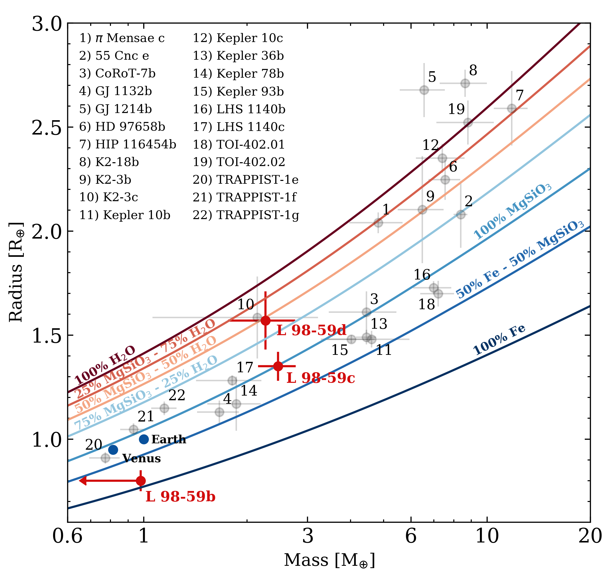
The planetary masses corresponding to the RV semi-amplitudes measured with our data are M⊕ (at 95% confidence), M⊕, and M⊕. 42 measure planet-star radius ratios (, , and ) from which they derive planetary radii of R⊕, R⊕, and R⊕. The measured planetary masses and radii result in constraints on the planets’ bulk densities of g cm-3, g cm-3, g cm-3 thus making the two outer planets consistent with bulk compositions that are dominated by rock as demonstrated in the planetary mass-radius plane in Fig. 5. Although the non-detection of prevents a precise value of its bulk density from being derived, the close proximity of L 98-59b to its host star and its intermediate size between that of Earth and Mars are evidence for its terrestrial nature (Owen & Wu 2013; Jin et al. 2014; Lopez & Fortney 2014; Chen & Rogers 2016; Lopez & Rice 2016; Owen & Wu 2017). Further constraints on may be realized as we note that the upper limit on g cm-3 from the 95% confidence interval of the marginalized posterior exceeds the bulk density of a pure iron ball the size of L 98-59b (12.2 g cm-3; Zeng & Sasselov 2013). This implies that the true RV semi-amplitude of L 98-59b is likely m s-1 and that the detection of will require much more stringent RV follow-up with an instrument whose performance on L 98-59 is similar to or better than HARPS, such as ESPRESSO (Pepe et al. 2010).
| 3-planet model plus GP activity | 3-planet model plus an untrained | |
| model trained on H | GP activity model | |
| Systemic velocity, [m s-1] | ||
| GP hyperparameters | ||
| Covariance amplitude, [m s-1] | ||
| Exponential timescale, [days] | ||
| Coherence, | ||
| Periodic timescale, [days] | ||
| Additive jitter, [m s-1] | ||
| Measured parameters | ||
| L 98-59b (TOI-175.03) | ||
| Orbital period, [days] | ||
| Time of mid-transit, [BJD-2,457,000] | ||
| Semi-amplitude, [m s-1]∗ | ||
| L 98-59c (TOI-175.01) | ||
| Orbital period, [days] | ||
| Time of mid-transit, [BJD-2,457,000] | ||
| Semi-amplitude, [m s-1] | ||
| L 98-59d (TOI-175.02) | ||
| Orbital period, [days] | ||
| Time of mid-transit, [BJD-2,457,000] | ||
| Semi-amplitude, [m s-1] | ||
| ln Bayesian evidence, | -411.5 | -410.3 |
| Derived parameters | ||
| L 98-59b (TOI-175.03) | ||
| Semi-major axis, [AU] | ||
| Equilibrium temperature, [K] | ||
| Bond albedo = 0 | ||
| Bond albedo = 0.3 | ||
| Planet radius, [R⊕]† | ||
| Planet mass, [M⊕]∗ | ||
| Bulk density, [g cm-3]∗ | ||
| Surface gravity, [m s-2]∗ | ||
| Escape velocity, [km s-1]∗ | ||
| Eccentricity, | ||
| L 98-59c (TOI-175.01) | ||
| Semi-major axis, [AU] | ||
| Equilibrium temperature, [K] | ||
| Bond albedo = 0 | ||
| Bond albedo = 0.3 | ||
| Planet radius, [R⊕]† | ||
| Planet mass, [M⊕] | ||
| Bulk density, [g cm-3] | ||
| Surface gravity, [m s-2] | ||
| Escape velocity, [km s-1] | ||
| Eccentricity, | ||
| L 98-59d (TOI-175.02) | ||
| Semi-major axis, [AU] | ||
| Equilibrium temperature, [K] | ||
| Bond albedo = 0 | ||
| Bond albedo = 0.3 | ||
| Planet radius, [R⊕]† | ||
| Planet mass, [M⊕] | ||
| Bulk density, [g cm-3] | ||
| Surface gravity, [m s-2] | ||
| Escape velocity, [km s-1] | ||
| Eccentricity, | ||
-
∗ Upper limit given by the 95% confidence interval.
-
† Planetary radii from 42.
-
‡ Upper limit given by the 95% confidence interval derived from the joint RV and dynamical stability analyses.
5 Dynamical Stability and Eccentricity Constraints
The presence of three planets in a compact configuration around L 98-59 provides a unique opportunity to provide additional constraints on the planets’ orbital eccentricities using stability criteria to limit the range of permissible eccentricities. 42 showed through dynamical simulations (assuming MAP planet mass predictions from Chen & Kipping 2017) that for initially circular orbits the system can be long-lived but as the initial eccentricities were increased to just 0.1, many of their simulated planetary systems became unstable in years. Using the planetary mass measurements and upper limits derived in this paper we can use dynamical simulations to constrain each planet’s eccentricity given that the system must remain stable for at least the duration of the simulation.
We proceed with deriving the fraction of stable systems as a function of each planet’s orbital eccentricity by simulating realizations of the L 98-59 planetary system and integrating each system forward in time using the WHFast symplectic integrator (Rein & Tamayo 2015) within the open-source REBOUND N-body package (Rein & Liu 2012). In each realization, the stellar mass is draw from M⊙ which in turn prescribes each planet’s initial semi-major axis when combined with its orbital period that are drawn from their marginalized posterior PDF from Sect. 4. 42 noted that despite having a period ratio of 2.02, the two outer planets are likely just wide of a resonant configuration such that we do not attempt to force the outer planet pair to converge towards a mean motion resonance in our dynamical simulations. Similarly to the orbital periods, each planet’s mass and orbital phase at are drawn from their marginalized posterior PDFs from Sect. 4. Orbital inclinations are drawn from the approximately Gaussian posterior PDFs reported in Table 2 of 42. The argument of periastron and longitude of the ascending node for each planet are both drawn from . Lastly, the orbital eccentricities of the planets in each realization are treated as free parameters and are drawn from where the upper eccentricity limit was chosen as any orbit that is initialized with will undergo an immediate orbit crossing in less than one orbital timescale.
Each simulated planetary system is integrated forward in time until one of the following stopping conditions is reached:
- 1.
Any pair of planets come within one mutual Hill radius:
(4) - 2.
Any planet that travels beyond the imposed maximum barycentric distance of 0.2 AU ().
- 3.
The integration reaches its stopping time of orbits of the outermost planet; years.
Simulations that are halted because of either of the former two stopping criteria are flagged as unstable systems and the corresponding initial eccentricities are ruled out due to instability. The remaining systems that survive until the end of the simulation are deemed stable. Note that due to the short duration of the simulations performed here compared to the expected age of L 98-59 (42, Gyr;), these simulations are not intended to provide a detailed overview of the system’s long-term stability but instead are used solely for the purpose of constraining the planetary eccentricities beyond that which can be measured by the RV data alone.
The fraction of stable systems as a function of each planet’s initial orbital eccentricity is shown in Fig. 6. The strong stability constraints on each planet’s eccentricity are evident as the majority of the 3-parameter space exhibits a stability fraction that is consistent with zero. In particular, for the two more massive planets in the system (i.e. L 98-59c and d), planetary systems for which or have a stability fraction of %. Conversely, a small fraction of planetary systems with can remain stable as the median mass of L 98-59b is only % of either of the other two planets and therefore its eccentricity has a reduced effect on the overall stability of the system (Barnes & Greenberg 2006).

The large fraction of initial eccentricity values that result in an unstable orbital configuration as seen in Fig. 6, provides constraints on the planets’ orbital eccentricity values. If initially we ignore the fractional stability criteria derived from our dynamical simulations, we can derive posterior PDFs of the orbital eccentricities from the PDFs of and obtained from our MCMC analysis (Fig. 2). The resulting posteriors are depicted in Fig. 7 and represent our measurements of from the RV data alone. Next, we treat the stability fraction as a function of each as an additional prior on and resample the posterior PDFs according to the stability fraction. That is, for each sample from the joint posterior derived from MCMC, the probability that that sample is retained is given by the stability fraction of simulated planetary systems with those eccentricity values . In this way high eccentricity values that cannot be ruled out by the MCMC analysis alone are frequently rejected because they often result in an unstable orbital configuration.

The resampled posteriors that account for system stability are compared to the MCMC only results in Fig. 7. The distinct narrowing of each posterior after including the stability criteria indicates that the joint RV stability data provide the strongest constraints on the orbital eccentricities of the planets in the compact L 98-59 system. From each set of posteriors we derive eccentricity upper limits at 95% confidence. The resulting upper limits from the RV data alone are , , and . By comparison, the inclusion of the stability criteria results in drastically improved upper limits of , , and . These measurements confirm that the planets in the L 98-59 compact planetary system all likely have eccentricities , a result that is consistent with similarly compact systems exhibiting low eccentricities (Hadden & Lithwick 2014; Van Eylen & Albrecht 2015) and the low dispersion in mutual inclinations in the system (42, ;).
6 Discussion & Conclusions
In this study we conducted an intensive HARPS RV follow-up campaign of the L 98-59 multi-planet system to characterize the masses of its three known transiting planets (42). We measure planet masses of the two outermost planets of M⊕ and M⊕ and derive an upper limit on the mass of the innermost planet of at 95% confidence. The resulting bulk densities of the two outer planets are roughly consistent with bulk terrestrial compositions (see Fig. 5) while the small size and small orbital separation place the innermost planet interior to the photoevaporation valley (Owen & Wu 2013; Jin et al. 2014; Lopez & Fortney 2014; Chen & Rogers 2016; Lopez & Rice 2016; Owen & Wu 2017) thus providing supporting evidence for its terrestrial nature as well. Confirmation of the terrestrial nature of L 98-59b will likely require additional RVs with a similar level of precision as our HARPS RVs to measure the semi-amplitude of L 98-59b at (Cloutier et al. 2018) given its expected semi-amplitude of 0.32 m s-1 (Chen & Kipping 2017).
With the precise RV planet masses presented in this study, L 98-59c and d add to the growing list of planets to directly contribute to the completion of the TESS level one science requirement of delivering the masses of fifty planets smaller than 4 R⊕. Furthermore, at 1.35 and 1.57 R⊕ respectively, L 98-59c and d are among the smallest TESS planets to have precisely measured masses via RV follow-up observations.
The nearby L 98-59 system of three terrestrial planets in a compact configuration within 7.5 days presents an ideal opportunity for comparative atmospheric planetology. To quantify the feasibility of detecting atmospheric signatures from the L 98-59 planets in transmission using JWST (assuming cloud-free atmospheres), we compute the transmission spectroscopy metric from Kempton et al. 2018 using the MAP planet parameters measured in this study. We find that TSM33 3 Assuming that 95% upper limit on from Table 4., TSM, and TSM. For L 98-59c and d this amounts to and times that of GJ 1132b (Dittmann et al. 2017; Bonfils et al. 2018), the previously ‘best’ prospect for the atmospheric characterization of a terrestrial-sized exoplanet from the pre-TESS era (Morley et al. 2017). Hence L 98-59c, and particularly L 98-59d, represent extremely promising targets for the atmospheric characterization of hot terrestrial exoplanets.
Similarly we compute the emission spectroscopy metric from Kempton et al. 2018 assuming that the planet day-side temperatures are equivalent to their equilibrium temperatures assuming an Earth-like albedo (i.e. ). We find ESM, ESM, ESM such that the L 98-59 planets are somewhat less favorable for emission spectroscopy characterization compared to GJ 1132b (ESM) although L 98-59c still represents a viable target for such observations. The disfavourability of the L 98-59 planets compared to GJ 1132b is largely due to the larger stellar radius of L 98-59. Nevertheless, the close proximity of L 98-59 ( pc) continues to make each of its known planets viable candidates for the characterization of hot terrestrial exoplanet atmospheres in emission if it can first be demonstrated on a slightly more favourable target such as GJ 1132b.
Regarding the prospect of the direct detection of the L 98-59 planets in reflected light using near-IR imagers on-board the next generation of extremely large telescopes, the planets’ small angular separations () make them difficult to resolve despite having modest planet-star contrasts ( respectively). Thus despite its close proximity, the orbital architecture of the known planets around L 98-59 is likely too compact for any of the planets to be directly imagable within the next decade.
Lastly, we emphasize that L 98-59 is slated to be re-observed by TESS within sectors 5, 8, 9, 10, 11, and 12. The extended baseline beyond the single 27 day field from sector 2 will provide opportunities to improve the orbital ephemerides and radii of the known planets and to continue to search for TTVs. If detected, TTV measurements could enable independent measurements of the planet masses for direct comparison to the RV results presented herein. The extended observational baseline may also enable the detection of additional planets at long orbital periods although the RVs presented herein do not show any significant evidence for such planets.
Acknowledgements.
R.C. is supported in part by the Natural Sciences and Engineering Research Council of Canada and acknowledges that this work was performed on land traditionally inhabited by the Wendat, the Anishnaabeg, Haudenosaunee, Metis, and the Mississaugas of the New Credit First Nation. N.A-D. acknowledges the support of FONDECYT project 3180063. X.B. acknowledges funding from the European Research Council under the ERC Grant Agreement n. 337591-ExTrA. J.S.J acknowledges support by FONDECYT grant 1161218 and partial support from CONICYT project Basal AFB-170002. This work is supported by the French National Research Agency in the framework of the Investissements d’Avenir program (ANR-15-IDEX-02), through the funding of the “Origin of Life” project of the Univ. Grenoble-Alpes. N.C.S was supported by FCT/MCTES through national funds and by FEDER - Fundo Europeu de Desenvolvimento Regional through COMPETE2020 - Programa Operacional Competitividade e Internacionalização by these grants: UID/FIS/04434/2019; PTDC/FIS-AST/32113/2017 & POCI-01-0145-FEDER-032113; PTDC/FIS-AST/28953/2017 & POCI-01-0145-FEDER-028953. Funding for the TESS mission is provided by NASA’s Science Mission directorate. We acknowledge the use of public TESS Alert data from pipelines at the TESS Science Office and at the TESS Science Processing Operations Center. This research has made use of the Exoplanet Follow-up Observation Program website, which is operated by the California Institute of Technology, under contract with the National Aeronautics and Space Administration under the Exoplanet Exploration Program. Resources supporting this work were provided by the NASA High-End Computing (HEC) Program through the NASA Advanced Supercomputing (NAS) Division at Ames Research Center for the production of the SPOC data products. This paper includes data collected by the TESS mission, which are publicly available from the Mikulski Archive for Space Telescopes (MAST).References
- Astudillo-Defru et al. (2017a) Astudillo-Defru, N., Delfosse, X., Bonfils, X., et al. 2017a, A&A, 600, A13
- Astudillo-Defru et al. (2017b) Astudillo-Defru, N., Díaz, R. F., Bonfils, X., et al. 2017b, A&A, 605, L11
- Astudillo-Defru et al. (2017c) Astudillo-Defru, N., Forveille, T., Bonfils, X., et al. 2017c, A&A, 602, A88
- Ballard (2019) Ballard, S. 2019, AJ, 157, 113
- Barclay et al. (2018) Barclay, T., Pepper, J., & Quintana, E. V. 2018, The Astrophysical Journal Supplement Series, 239, 2
- Barnes & Greenberg (2006) Barnes, R. & Greenberg, R. 2006, ApJ, 647, L163
- Benedict et al. (2016) Benedict, G. F., Henry, T. J., Franz, O. G., et al. 2016, AJ, 152, 141
- Bonfils et al. (2018) Bonfils, X., Almenara, J. M., Cloutier, R., et al. 2018, A&A, 618, A142
- Brahm et al. (2018) Brahm, R., Espinoza, N., Jordán, A., et al. 2018, arXiv e-prints [arXiv:1811.02156]
- Cañas et al. (2019) Cañas, C. I., Stefansson, G., Monson, A. J., et al. 2019, arXiv e-prints [arXiv:1902.09710]
- Chen & Rogers (2016) Chen, H. & Rogers, L. A. 2016, ApJ, 831, 180
- Chen & Kipping (2017) Chen, J. & Kipping, D. 2017, ApJ, 834, 17
- Cloutier (2018) Cloutier, R. 2018, arXiv e-prints [arXiv:1812.08145]
- Cloutier et al. (2017) Cloutier, R., Astudillo-Defru, N., Doyon, R., et al. 2017, A&A, 608, A35
- Cloutier et al. (2019) Cloutier, R., Astudillo-Defru, N., Doyon, R., et al. 2019, A&A, 621, A49
- Cloutier et al. (2018) Cloutier, R., Doyon, R., Bouchy, F., & Hébrard, G. 2018, AJ, 156, 82
- Cutri et al. (2003) Cutri, R. M., Skrutskie, M. F., van Dyk, S., et al. 2003, 2MASS All Sky Catalog of point sources.
- Cutri et al. (2013) Cutri, R. M., Wright, E. L., Conrow, T., et al. 2013, Explanatory Supplement to the AllWISE Data Release Products, Tech. rep.
- Desort et al. (2007) Desort, M., Lagrange, A.-M., Galland, F., Udry, S., & Mayor, M. 2007, A&A, 473, 983
- Dittmann et al. (2017) Dittmann, J. A., Irwin, J. M., Charbonneau, D., et al. 2017, Nature, 544, 333
- Dragomir et al. (2019) Dragomir, D., Teske, J., Gunther, M. N., et al. 2019, arXiv e-prints [arXiv:1901.00051]
- Dumusque et al. (2019) Dumusque, X., Turner, O., Dorn, C., et al. 2019, arXiv e-prints, arXiv:1903.05419
- Duncan et al. (1991) Duncan, D. K., Vaughan, A. H., Wilson, O. C., et al. 1991, ApJS, 76, 383
- Espinoza et al. (2019) Espinoza, N., Brahm, R., Henning, T., et al. 2019, arXiv e-prints [arXiv:1903.07694]
- Evans et al. (2018) Evans, D. W., Riello, M., De Angeli, F., et al. 2018, A&A, 616, A4
- Fabrycky et al. (2014) Fabrycky, D. C., Lissauer, J. J., Ragozzine, D., et al. 2014, ApJ, 790, 146
- Ford (2006) Ford, E. B. 2006, ApJ, 642, 505
- Foreman-Mackey et al. (2013) Foreman-Mackey, D., Hogg, D. W., Lang, D., & Goodman, J. 2013, PASP, 125, 306
- Gaia Collaboration et al. (2018) Gaia Collaboration, Brown, A. G. A., Vallenari, A., et al. 2018, A&A, 616, A1
- Gandolfi et al. (2018) Gandolfi, D., Barragán, O., Livingston, J. H., et al. 2018, A&A, 619, L10
- Giles et al. (2017) Giles, H. A. C., Collier Cameron, A., & Haywood, R. D. 2017, MNRAS, 472, 1618
- Gomes da Silva et al. (2012) Gomes da Silva, J., Santos, N. C., Bonfils, X., et al. 2012, A&A, 541, A9
- Hadden & Lithwick (2014) Hadden, S. & Lithwick, Y. 2014, ApJ, 787, 80
- Henden et al. (2016) Henden, A. A., Templeton, M., Terrell, D., et al. 2016, VizieR Online Data Catalog, 2336
- Huang et al. (2018a) Huang, C. X., Burt, J., Vanderburg, A., et al. 2018a, arXiv e-prints, arXiv:1809.05967
- Huang et al. (2018b) Huang, C. X., Shporer, A., Dragomir, D., et al. 2018b, arXiv e-prints, arXiv:1807.11129
- Jenkins et al. (2016) Jenkins, J. M., Twicken, J. D., McCauliff, S., et al. 2016, in Proc. SPIE, Vol. 9913, Software and Cyberinfrastructure for Astronomy IV, 99133E
- Jin et al. (2014) Jin, S., Mordasini, C., Parmentier, V., et al. 2014, ApJ, 795, 65
- Jones et al. (2018) Jones, M. I., Brahm, R., Espinoza, N., et al. 2018, arXiv e-prints [arXiv:1811.05518]
- Kempton et al. (2018) Kempton, E. M.-R., Bean, J. L., Louie, D. R., et al. 2018, ArXiv e-prints [arXiv:1805.03671]
- Kipping et al. (2019) Kipping, D., Nesvorný, D., Hartman, J., et al. 2019, arXiv e-prints [arXiv:1902.03900]
- Kostov et al. (2019) Kostov, V. B., Schlieder, J. E., Barclay, T., et al. 2019, arXiv e-prints, arXiv:1903.08017
- Li et al. (2019) Li, J., Tenenbaum, P., Twicken, J. D., et al. 2019, Publications of the Astronomical Society of the Pacific, 131, 024506
- Lindegren & Dravins (2003) Lindegren, L. & Dravins, D. 2003, A&A, 401, 1185
- Lindegren et al. (2018) Lindegren, L., Hernández, J., Bombrun, A., et al. 2018, A&A, 616, A2
- Lissauer et al. (2011) Lissauer, J. J., Ragozzine, D., Fabrycky, D. C., et al. 2011, ApJS, 197, 8
- Lopez & Fortney (2014) Lopez, E. D. & Fortney, J. J. 2014, ApJ, 792, 1
- Lopez & Rice (2016) Lopez, E. D. & Rice, K. 2016, ArXiv e-prints [arXiv:1610.09390]
- Louie et al. (2018) Louie, D. R., Deming, D., Albert, L., et al. 2018, PASP, 130, 044401
- Lovis & Pepe (2007) Lovis, C. & Pepe, F. 2007, A&A, 468, 1115
- Mann et al. (2019) Mann, A. W., Dupuy, T., Kraus, A. L., et al. 2019, ApJ, 871, 63
- Mann et al. (2015) Mann, A. W., Feiden, G. A., Gaidos, E., Boyajian, T., & von Braun, K. 2015, ApJ, 804, 64
- Mayor et al. (2003) Mayor, M., Pepe, F., Queloz, D., et al. 2003, The Messenger, 114, 20
- Ment et al. (2019) Ment, K., Dittmann, J. A., Astudillo-Defru, N., et al. 2019, AJ, 157, 32
- Morley et al. (2017) Morley, C. V., Kreidberg, L., Rustamkulov, Z., Robinson, T., & Fortney, J. J. 2017, ApJ, 850, 121
- Muirhead et al. (2018) Muirhead, P. S., Dressing, C. D., Mann, A. W., et al. 2018, AJ, 155, 180
- Nelson et al. (2018) Nelson, B. E., Ford, E. B., Buchner, J., et al. 2018, ArXiv e-prints, arXiv:1806.04683
- Newton et al. (2016) Newton, E. R., Irwin, J., Charbonneau, D., et al. 2016, ApJ, 821, 93
- Nielsen et al. (2019) Nielsen, L. D., Bouchy, F., Turner, O., et al. 2019, A&A, 623, A100
- Owen & Wu (2013) Owen, J. E. & Wu, Y. 2013, ApJ, 775, 105
- Owen & Wu (2017) Owen, J. E. & Wu, Y. 2017, ApJ, 847, 29
- Pepe et al. (2010) Pepe, F. A., Cristiani, S., Rebolo Lopez, R., et al. 2010, in Proc. SPIE, Vol. 7735, Ground-based and Airborne Instrumentation for Astronomy III, 77350F
- Perrakis et al. (2014) Perrakis, K., Ntzoufras, I., & Tsionas, E. G. 2014, 77, 54
- Queloz et al. (2001) Queloz, D., Henry, G. W., Sivan, J. P., et al. 2001, A&A, 379, 279
- Quinn et al. (2019) Quinn, S. N., Becker, J. C., Rodriguez, J. E., et al. 2019, arXiv e-prints, arXiv:1901.09092
- Rein & Liu (2012) Rein, H. & Liu, S. F. 2012, A&A, 537, A128
- Rein & Tamayo (2015) Rein, H. & Tamayo, D. 2015, MNRAS, 452, 376
- Ricker et al. (2015) Ricker, G. R., Winn, J. N., Vanderspek, R., et al. 2015, Journal of Astronomical Telescopes, Instruments, and Systems, 1, 014003
- Rodriguez et al. (2019) Rodriguez, J. E., Quinn, S. N., Huang, C. X., et al. 2019, arXiv e-prints, arXiv:1901.09950
- Stassun et al. (2018) Stassun, K. G., Oelkers, R. J., Pepper, J., et al. 2018, AJ, 156, 102
- Sullivan et al. (2015) Sullivan, P. W., Winn, J. N., Berta-Thompson, Z. K., et al. 2015, ApJ, 809, 77
- Twicken et al. (2018) Twicken, J. D., Catanzarite, J. H., Clarke, B. D., et al. 2018, Publications of the Astronomical Society of the Pacific, 130, 064502
- Van Eylen & Albrecht (2015) Van Eylen, V. & Albrecht, S. 2015, ApJ, 808, 126
- Vanderburg et al. (2016) Vanderburg, A., Plavchan, P., Johnson, J. A., et al. 2016, MNRAS, 459, 3565
- Vanderspek et al. (2019) Vanderspek, R., Huang, C. X., Vanderburg, A., et al. 2019, ApJ, 871, L24
- Wang et al. (2019) Wang, S., Jones, M., Shporer, A., et al. 2019, AJ, 157, 51
- Zechmeister & Kürster (2009) Zechmeister, M. & Kürster, M. 2009, A&A, 496, 577
- Zeng & Sasselov (2013) Zeng, L. & Sasselov, D. 2013, PASP, 125, 227